Kinematic Calibration of a Space Manipulator Based on Visual Measurement System with Extended Kalman Filter

Abstract

The calibration of kinematic parameters has been widely used to improve the pose (position and orientation) accuracy of the robot arm. Intelligent measuring equipment with high accuracy is usually provided for the industrial manipulator. Unfortunately, large noise exists in the vision measurement system, which is provided for space manipulators. To overcome the adverse effect of measuring noise and improve the optimality of calibrating time, a calibration method based on extended Kalman filter (EKF) for space manipulators is proposed in this paper. Firstly, the identification model based on the Denavit–Hartenberg (D-H) modeling method is established. Then, the camera which is rigidly attached to the end-effector takes pictures of a calibration board that is settled around the manipulator. The actual pose of the end-effector is calculated based on the pictures of the calibration board. Subsequently, different data between the actual pose and theoretical pose as input, whilst error parameters are estimated by EKF and compensated in the kinematic algorithm. The simulation result shows that the pose accuracy has been improved by approximately 90 percent. Compared with the calibration method of the least squares estimate (LSE), EKF is beneficial to further optimize the calibrating time with a faster computation speed and ensure the stability of the calibration.

1. Introduction

As a core piece of equipment, the space robot arm undertakes several tasks such as equipment assembly and maintenance, spacecraft docking and transferring, and assisting astronauts with extra-vehicular activities (EVAs) [1,2]. On account of complicated tasks and polytropic space environments, space manipulators must be flexible and autonomous to achieve the desired configurations with high accuracy [3]. However, the tolerances generated during the manufacturing and assembly of the manipulator can make a difference in the geometric structure of the manipulator. Apart from that, changes in the environment and the abrasion of the mechanical mechanism due to long-term work are also important factors. Because of the geometric structure difference, the actual kinematic parameters of a robot deviate from their nominal values, which are referred to as kinematic errors.

Kinematic errors generated during production and assembly can be calibrated by ground experiments before launching on a rocket. However, due to the strong shocks and vibrations during the launch and flight of the rocket, the space manipulator, which has already been calibrated by ground experiments, requires kinematic calibration before entering on duty [4]. Kinematics calibration is defined as the process of enhancing robot pose (position and orientation) accuracy by modifying its kinematic model, which depicts the relationship between Cartesian space and the robot’s joint space without changing the robot’s hardware configurations [5]. The kinematic calibration of the manipulator is divided into four steps: (1) Modeling the manipulator; (2) Measuring the pose of the end-effector; (3) Identification of the kinematic error; and (4) Compensation for the kinematic model.

Completeness, minimality, and model continuity are three indexes to evaluate a modeling method of the manipulator [6]. The D-H modeling method is one of the most widely used modeling methods. However, when it is used to describe the joints of parallel structures, small changes in the joint axis attitude can bring large changes in the D-H parameters. Thus, it does not apply to the kinematic calibration of manipulators in particular configurations [7]. Veitschegger and Wu [8] proposed an improved method based on the D-H kinematic modeling method, which solved the discontinuity problem by adding a torsion angle β parameter to the conventional D-H model. However, both the identification models of the improved method and the conventional method have a non-minimality problem that exists in redundant parameters. Okamura et al. [9] proposed a robot modeling method based on the product of exponentials (POE), and He et al. [10] derived an explicit form of the identification model based on the POE method. The method has shown that parameters of the identification model smoothly vary with small changes in joint axes in the experiments, and has been intensively researched by many researchers [11,12,13,14,15].

The modification of the kinematic model decides on the result of the kinematic identification algorithm, which calculates kinematic errors based on manipulator configuration and detected poses. The kinematic identification algorithm is the core part of calibration and can be divided into model-based and nonparametric algorithms. Identification models that represent a relationship between Cartesian space and joint space small errors are the foundation of the model-based kinematic identification algorithm. Conventional calibration commonly uses the model-based algorithm for the identification of, e.g., LSE. The nonparametric kinematic calibration algorithm is a new technique based on intelligent algorithms which commonly requires a huge quantity of experimental data rather than the kinematic model. The accuracy and stability of the nonparametric kinematic calibration method are reliant on the parameters of the intelligent algorithm [6].

The least squares method is the most convenient method and is commonly used to calibrate industrial manipulators. This method is simple and effective but is very sensitive to measuring noise. Industrial calibration utilizes several measurement techniques such as coordinate measuring machines and laser tracking interferometer systems. However, these systems are very expensive and not user-friendly [16,17,18]. The Levenberg–Marquardt (LM) algorithm [19,20,21] is a Newton iterative algorithm based on the LSE. This algorithm is friendly to the user and could circumvent the singularity problem of the D-H model, but it is prone to generating suboptimal results. Du et al. [22,23] used the EKF and the unscented Kalman filter (UKF), respectively, to calibrate the manipulator. The two methods provide superior results with high accuracy and a quicker computation time compared to the (LSE), but these are susceptible to the local optimal problem. Then, Du et al. [24] compared UKF with EKF and the result shows that the calibration accuracy of UKF and EKF is similar, but UKF requires fewer original data. The UKF and the EKF are well-known nonlinear state estimation methods and have been compared by many research groups, with mixed conclusions reported [25,26,27]. Sage–Husa adaptive Kalman filtering (Sage-Husa AKF) algorithm can estimate the statistical properties of the noise, but the calculation is complex [28,29]. Ma et al. [30] proposed a calibration method based on maximum likelihood estimation (MLE). This approach is intuitive and straightforward in practice but requires a large quantity of experimental data. The application of the metaheuristic algorithm in calibration has become a research hotspot in recent years. Genetic algorithm (GA) [31], particle swarm optimization (PSO) [32], quantum-behaved PSO (QPSO) [33], and artificial neural network (ANN) [34,35,36] have been used to calibrate manipulators with good results. However, the common problem with these algorithms is that they can fall into a local optimum with slow convergence. Additionally, in the calibrations of the ANN, the training data used obtained from the idealized inverse kinematics of the robot is inaccurate. All methods are summarized in

Table 1. Calibration algorithms and their advantages and disadvantages.

Algorithm	Advantage	Disadvantage	Reference
LSE	Simple structure; widely used.	It is sensitive to measurement noise and requires sensors with high precision.	[16,17,18]
LM	It is friendly to the user and could circumvent the singularity problem of the D-H model.	It is prone to generating suboptimal results.	[19,20,21]
EKF	The calculation speed is fast, the effect is obvious, and the measurement noise can be filtered.	The effect is unstable and the statistical property of noise needs to be known.	[22,23]
UKF	The effect is obvious, fewer original data may be required, and the measurement noise can be filtered.	The effect is unstable and the statistical property of noise needs to be known.	[24,25,26,27]
Sage–Husa AKF	It can deal with time-varying noise problem.	The calculation is complex and the effect is unstable.	[28,29]
MLE	It is intuitive and straightforward in practice.	A large quantity of experimental data is required.	[30]
GA	It is reliable, numerically precise, and the kinematic model of the manipulator is not required.	It is very sensitive to parameter change and computations are huge.	[31]
PSO	It has simple structure, and it is easy to implement.	It can fall into a local optimum with slow convergence.	[32]
QPSO	It has simple structure, and it is easy to implement.	It can fall into a local optimum with slow convergence.	[33]
ANN	It is a powerful tool for treating mathematically ill-defined systems, and the kinematic model of the manipulator is not required.	Suffers from dependency on procedure and excessive tuning of adaptive gains.	[34,35,36]

.

There are many activities to be accomplished by the Chinese space manipulator (CSM), such as aided cabin docking and carrying out scientific experiments. The CSM system includes the mechanical arm, the in-cabin operation equipment and the remote operation equipment settling in the ground. The mechanical arm consists of seven joints, two end-effectors, two arms, controllers, and cameras [37,38]. CSM measures the pose of the end-effector with a vision system. A camera is attached to the end-effector, which is referred to as an eye-in-hand, for photographing the calibration board which is settled around the manipulator and fixed on the outside of the space station. During the manipulator moving, the end-effector must keep the calibration board in the field of view of the camera. In comparison to the measurement equipment regularly used in ground experiments, the vision system a with large measuring noise requires an effective calibration method that can eliminate noise interference.

The simple structure and excellent computing efficiency of the Kalman filter has led to wide adoption since being proposed. In this paper, the EKF is used to calibrate the space manipulator in order to solve the problem of high noise. The contributions are as follows: firstly, the CSM kinematics simulation platform is built, and the control noise is added into the kinematics calculation of the manipulator. The simulation model of the CSM vision measurement system is established, and the pose data of the end-effector those of the including measurement noise are simulated. The adverse effects of two kinds of noise are simulated. The existing LSE calibration effect of the space manipulator is greatly affected by noise. In this paper, EKF is used for calibration and compared with LSE. The simulation performance of EKF is analyzed.

This paper is organized as follows. Section II presents the kinematic model and error model of the space manipulator. Section III introduces the visual measurement system of the space manipulator and the discrimination principle based on the extended Kalman filter method. Experiments are conducted in Section IV and Section V analyzes and gives conclusions based on the experimental results.

2. Materials and Methods

In this study, the kinematic model and identification model of the manipulator are built based on the D-H method, which has been used in the China space manipulator, and the DH model of the manipulator is as follows.

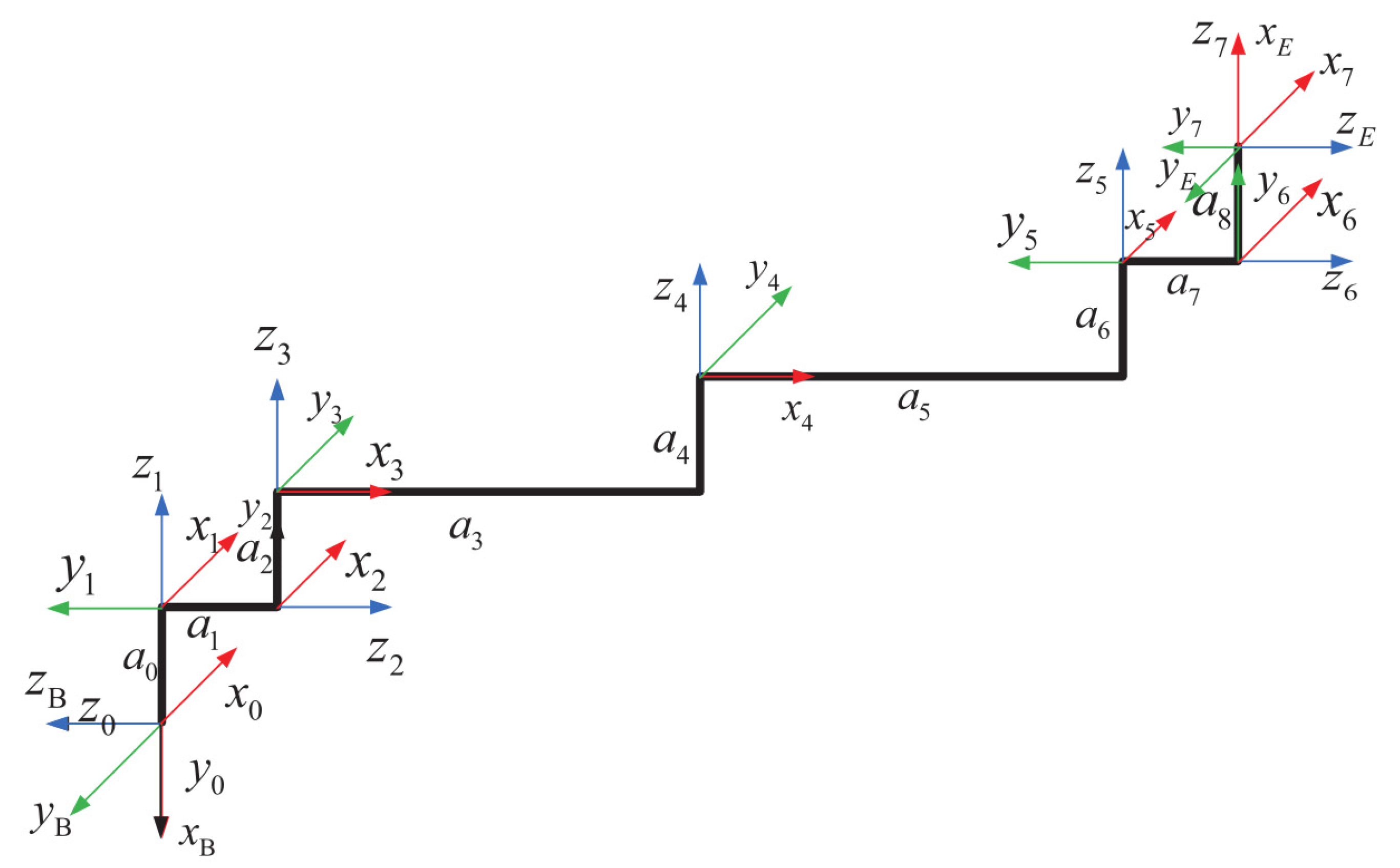
2.1. DH Coordinate System

The Chinese space station has two manipulators, which are both Space Station Remote Manipulator System (SSRMS) configuration space manipulators with link offset at the shoulder and wrist and one redundant degree of freedom. The manipulator configuration is R–Y–P–P–P–Y–R. The joint coordinate systems are depicted in Figure 1.

Due to the offset at the shoulder and wrist of the manipulator, the linkage length of joint 4 and joint 5 is not equal to 0. The D-H parameters of each joint are shown in

Table 2. The parameter list of the kinematic model.

Link i	${\mathit{a}}_{\mathit{i}-1}\left(\mathbf{m}\right)$	${\mathit{\alpha }}_{\mathit{i}-1}\left(\text{°}\right)$	${\mathit{d}}_{\mathit{i}}\left(\mathbf{m}\right)$	${\mathit{\theta }}_{\mathit{i}}\left(\text{°}\right)$
0	0	0	0	−90
1	0	90	l0	0
2	0	90	l1	0
3	0	−90	l2	−90
4	l3	0	l4	0
5	l5	0	l6	90
6	0	90	l7	0
7	0	−90	l8	0
E	0	90	0	90

Note: $a_{i-1}$ is the length of the link, which is defined as the distance from $z_{i-1}$ to $z_i$ measured along $x_{i-1}$ positive direction; ${\alpha }_{i-1}$ is the torsion angle of the link, which is defined as the angle from $z_{i-1}$ to $z_i$ measured in the $x_{i-1}$ positive direction; $d_i$ is the offset distance of the link, which is defined as the distance from $x_{i-1}$ to $x_i$ measured along the $z_i$ positive direction; and ${\theta }_i$ is the rotation angle of link, which is defined as the angle from $x_{i-1}$ to $x_i$ measured along the $z_i$ positive direction. Coordinate ${\sum }_E$ is the tool frame.

.

2.2. Forward and Inverse Kinematic Model

The positional relationship between adjacent link coordinate systems is represented by the homogeneous transformation matrix ${}_i{}^{i-1}\mathit{T}$. That is

$${}_i{}^{i-1}\mathit{T}=\left[\begin{array}{cccc}c{\theta }_i& -s{\theta }_i& 0& {\alpha }_{i-1}\\ s{\theta }_{i}c{\alpha }_{i-1}& c{\theta }_{i}c{\alpha }_{i-1}& -s{\alpha }_{i-1}& -s{\alpha }_{i-1}{d}_i\\ s{\theta }_{i}s{\alpha }_{i-1}& c{\theta }_{i}s{\alpha }_{i-1}& c{\alpha }_{i-1}& c{\alpha }_{i-1}{d}_i\\ 0& 0& 0& 1\end{array}\right]=\left[\begin{array}{cccc}{n}_{x,i}^{i-1}& o_{x,i}^{i-1}& a_{x,i}^{i-1}& p_x\\ n_{y,i}^{i-1}& o_{y,i}^{i-1}& a_{y,i}^{i-1}& p_y\\ n_{z,i}^{i-1}& o_{z,i}^{i-1}& a_{z,i}^{i-1}& p_z\\ 0& 0& 0& 1\end{array}\right]$$

(1)

where c(.) = cos(.), s(.) =sin(.). Multiplying the homogeneous matrix, we obtain

$${}_E{}^B\mathit{T}={}_1{}^B\mathit{T}{}_2{}^1\mathit{T}{}_3{}^2\mathit{T}{}_4{}^3\mathit{T}{}_5{}^4\mathit{T}{}_6{}^5\mathit{T}{}_7{}^6\mathit{T}{}_E{}^7\mathit{T}$$

(2)

Each D-H parameter of the manipulator is brought into Equation (2) to obtain the end-effector poses. Equation (2) is the forward kinematic equation of the manipulator.

The inverse kinematic solution requires one of the ${\theta }_1$, ${\theta }_2$, ${\theta }_6$, ${\theta }_7$ to be fixed. In this study, we picked ${\theta }_2$ as the fixed joint value because it can lock the direction of the plane (arm plane) containing the two longest links (upper arm and forearm). This operation can significantly reduce the probability of collision with the obstacle due to the large change in the manipulator configuration during the working process.

Since the range of activity of the joint angle is [−300°, +300°], which can rotate for more than one week, there are more than 8 sets of solutions for the inverse kinematics. In the results of the inverse kinematics calculation, we follow the principle of minimum joint rotation angle to select the optimal solution. Define $u={\theta }_2$, $\mathit{x}=[{\theta }_1,{\theta }_2,{\theta }_3,{\theta }_4,{\theta }_5,{\theta }_6,{\theta }_7]$. Then, the forward kinematic equation can be expressed as

$$f(\mathit{x},u)=\mathit{T}$$

(3)

The inverse kinematics can be expressed as

$$\mathit{x}=ikine(u,\mathit{T},{\mathit{x}}_0)$$

(4)

where ${\mathit{x}}_0$ is the initial configuration of the manipulator, $u$ is the selected fixed joint angle parameter, and $\mathit{T}$ is the target pose matrix of the end-effector in the base coordinate system.

2.3. Identification Model

There are several causes of end-effector pose problems, including manufacturing faults, assembly errors, and link deformation. It is impractical to identify all these factors affecting end-effector pose accuracy. We have to build an identification model representing the relationship between manipulator joint parameters and end-effector poses for attributing the impact of all error sources to the kinematic errors of each joint.

First, the identification model of the single joint is constructed.

$${}_i{}^{i-1}\mathit{T}{}^R={}_i{}^{i-1}\mathit{T}{}^N+d{}_i{}^{i-1}\mathit{T}$$

(5)

In Equation (5), ${}_i{}^{i-1}\mathit{T}{}^R$ is the actual homogeneous matrix of the i-th joint, ${}_i{}^{i-1}\mathit{T}{}^N$ is the theoretical homogeneous matrix of the i-th joint, and $d{}_i{}^{i-1}\mathit{T}{}^R$ is the error matrix between the actual homogeneous matrix and the ideal homogeneous matrix, which is called the micro-movement matrix. According to the differentiation theorem, we have

$$d{}_i{}^{i-1}\mathit{T}=\frac{\partial {}_i{}^{i-1}\mathit{T}{}^N}{\partial {\theta }_i}\Delta {\theta }_i+\frac{\partial {}_i{}^{i-1}\mathit{T}{}^N}{\partial d_i}\Delta d_i+\frac{\partial {}_i{}^{i-1}\mathit{T}{}^N}{\partial a_i}\Delta a_i+\frac{\partial {}_i{}^{i-1}\mathit{T}{}^N}{\partial {\alpha }_i}\Delta {\alpha }_i$$

(6)

where $\frac{\partial {}_i{}^{i-1}\mathit{T}{}^N}{\partial {\theta }_i}$, $\frac{\partial {}_i{}^{i-1}\mathit{T}{}^N}{\partial d_i}$, $\frac{\partial {}_i{}^{i-1}\mathit{T}{}^N}{\partial a_i}$, $\frac{\partial {}_i{}^{i-1}\mathit{T}{}^N}{\partial {\alpha }_i}$, respectively, are the partial derivatives of ${}_i{}^{i-1}\mathit{T}{}^N$ parameters $\theta$, $d$, $a$, $\alpha$ and $\Delta {\theta }_i$, $\Delta d_i$, $\Delta a_i$, $\Delta {\alpha }_i$ are the error of the i-th joint parameters.

$$\frac{\partial {}_i{}^{i-1}\mathit{T}{}^N}{\partial {\theta }_i}=D_{\theta i}{}_i{}^{i-1}\mathit{T}{}^N$$

The matrix ${}_i{}^{i-1}\mathit{T}{}^N$ is extracted from the results of the partial derivatives of the $\theta$, wherein $D_{\theta i}$ is called the coefficient matrix of the small change $\theta$. Performing the same operation on the remaining three partial derivative results yields

$$d{}_i{}^{i-1}\mathit{T}=\delta {}_i{}^{i-1}\mathit{T}\cdot {}_i{}^{i-1}\mathit{T}{}^N$$

(7)

where $\delta {}_i{}^{i-1}\mathit{T}=D_{\theta i}\Delta {\theta }_i+D_{di}\Delta d_i+D_{ai}\Delta a_i+D_{\alpha i}\Delta {\alpha }_i$. $\delta {}_i{}^{i-1}\mathit{T}$ is called the micro-movement rate of the transformation matrix and characterizes the relationship between the micro-movement matrix and the theoretical transformation matrix.

Based on the differential motion of the joint, the analysis of the result of Equation (7) is shown as

$${\mathit{e}}_i^E={\mathit{F}}_{i+1}^E\mathbf{·}{G}_i\mathbf{·}{\Delta }_i$$

(8)

$${\mathit{F}}_{i+1}^E=\left[\begin{array}{cc}\begin{array}{ccc}{n}_{x,i+1}^E& n_{y,i+1}^E& n_{z,i+1}^E\\ o_{x,i+1}^E& o_{y,i+1}^E& o_{z,i+1}^E\\ a_{x,i+1}^E& a_{y,i+1}^E& a_{z,i+1}^E\end{array}& \begin{array}{ccc}{\left(p_{i+1}^E\times n_{i+1}^E\right)}_x& {\left(p_{i+1}^E\times n_{i+1}^E\right)}_y& {\left(p_{i+1}^E\times n_{i+1}^E\right)}_z\\ {\left(p_{i+1}^E\times o_{i+1}^E\right)}_x& {\left(p_{i+1}^E\times o_{i+1}^E\right)}_y& {\left(p_{i+1}^E\times o_{i+1}^E\right)}_z\\ {\left(p_{i+1}^E\times a_{i+1}^E\right)}_x& {\left(p_{i+1}^E\times a_{i+1}^E\right)}_y& {\left(p_{i+1}^E\times a_{i+1}^E\right)}_z\end{array}\\ 0& \begin{array}{ccc}{n}_{x,i+1}^E& n_{y,i+1}^E& n_{z,i+1}^E\\ o_{x,i+1}^E& o_{y,i+1}^E& o_{z,i+1}^E\\ a_{x,i+1}^E& a_{y,i+1}^E& a_{z,i+1}^E\end{array}\end{array}\right]$$

where ${\mathit{e}}_i^E={[\begin{array}{ccc}d{x}_i^E& d{y}_i^E& \begin{array}{cccc}d{z}_i^E& \delta x_i^E& \delta y_i^E& \delta z_i^E\end{array}\end{array}]}^T$, ${\Delta }_i={[\begin{array}{ccc}\Delta {\theta }_i& \Delta d_i& \begin{array}{cc}\Delta a_i& \Delta {\alpha }_i\end{array}\end{array}]}^T$,$G_i=[D_{\theta i},D_{di},D_{ai},D_{\alpha i}]$. ${\mathit{e}}_i^E$ is the error caused by the i-th joint parameter error on the end poses. ${\mathit{F}}_{i+1}^E$ is the transformation matrix of the coordinate system. The reference frame of the end pose error is originally the coordinate system ${\sum }_{i+1}$, which has changed into the coordinate system ${\sum }_E$ by multiplying ${\mathit{F}}_{i+1}^E$. By changing the coordinate system, the errors caused by each joint to the end-effector poses can be linearly added together.

${\Delta }_i$ is the error of i-th joint parameters. This gives the final error pose of the manipulator, i.e.,

$$\mathit{e}={\displaystyle \mathit{\sum }_{i=1}^n{\mathit{e}}_i^E}={\displaystyle \mathit{\sum }_{i=1}^n{\mathit{F}}_i^E\mathbf{·}{\mathit{G}}_i\mathbf{·}{\mathbf{\Delta }}_i}$$

(9)

The mapping connection between the kinematic errors and the error poses of the end-effector is described in Equation (9). The pose error of the end-effector in various configurations is measured, and the error of the joint parameters could be calculated based on the identification model.

3. Identification of Kinematic Errors

The D-H parameters of the space manipulator are measured by a vision system and handled by the EKF to identify the kinematic error.

3.1. End-Effector Pose Acquisition

The China space manipulator is equipped with eye-in-hand cameras at the head and tail, which support a vision system to take pictures of the calibration board. The manipulator moves according to the planned configuration and takes pictures of the calibration board from different angles. These pictures correspond to the configurations and the physical dimensions of the black and white grids of the calibration board are known, as shown in Figure 2. According to the Zhang Zhengyou model [39], the real pose of the end-effector in Cartesian space could be identified by handling the pictures of the calibration board.

$$s\tilde{\mathit{m}}=\mathit{A}[Rt]\tilde{\mathit{M}}$$

(10)

Equation (10) defines the mapping connection between 2D coordinates in the calibration board pictures and 3D coordinates in Cartesian space, while Figure 3 depicts a calibration board. The coordinate of a 2D point in the calibration board pictures is denoted by m,$\mathit{m}={[v,w]}^T$. The origin of the Cartesian spatial coordinate system is fixed in the upper left corner of the calibrated board, and the calibration board plane is used as the XOY plane, with the x axis and y axis parallel to the edges of the checkerboard grid, respectively. The coordinate of a point in the Cartesian space is denoted by $\mathit{M}$,$\mathit{M}={[X,Y,Z]}^T$. In Equation (10), s is an arbitrary scale factor, and we use $\tilde{x}$ to denote the augmented vector by adding 1 as the last element: $\tilde{\mathit{m}}={[v,w,1]}^T$ and $\tilde{\mathit{M}}={[X,Y,Z,1]}^T$, and R and t denotes the extrinsic parameters of rotation and translation which relate the world coordinate system to the camera coordinate system. A is the camera intrinsic matrix,

$$\mathit{A}=\left[\begin{array}{ccc}\alpha & c& u_0\\ 0& \beta & v_0\\ 0& 0& 1\end{array}\right]$$

The solution to Equation (10) is more complex, and the process is discussed in detail in reference [40]. According to the Zhang Zhengyou model, the pictures of the calibration board photographed by the eye-in-hand camera are used to calculate the actual pose of the manipulator end-effector in Cartesian space. The position of the eye-in-hand camera in the manipulator is shown in Figure 3.

3.2. Identification Algorithm

KF is commonly used to remove the interference of measurement noise and predict the future state of the system. The technique brings the idea of state space into the stochastic estimating theory. The state equation, the observation equation, and the white noise excitation need to be known. KF could predict the missing information based on limited and indirect measurement data under the impact of noise, and the future state information could also be predicted based on historical data. The technique has been utilized for missile guidance, flood forecasting, and predicting the paths of stellar movements [41]. The conventional KF primarily examines linear systems. However, the EKF could effectively decrease nonlinear mistakes in the identification process for the identification model of the manipulator.

For the identification of kinematic errors, the pose error of the end-effector needs to provide for the EKF. After measuring the actual pose of the end-effector, the difference between the actual and the theoretical pose could be obtained.

Since each joint has four joint variables, the 7-degree-of-freedom robot arm has 28 joint variables. In the identification algorithm of the kinematic error, the state y contains 28 variables of 7 joints, $\mathit{y}={[\begin{array}{cccc}{\mathit{y}}_1& {\mathit{y}}_2& \begin{array}{cccc}{\mathit{y}}_3& {\mathit{y}}_4& {\mathit{y}}_5& {\mathit{y}}_6\end{array}& {\mathit{y}}_7\end{array}]}^T$. ${\mathit{y}}_i$ is the i-th joint variable, ${\mathit{y}}_i=[\begin{array}{cccc}\Delta {\theta }_i& \Delta {\alpha }_i& \Delta a_i& \Delta d_i\end{array}]$.

$${\widehat{\mathit{y}}}_{k+1|k}={\widehat{\mathit{y}}}_{k|k}$$

(11)

$$\mathit{P}{=}_{k+1|k}\mathit{P}{+}_{k|k}\mathit{Q}$$

(12)

According to EKF, Equations (11) and (12) are the prediction process of the system state in round k iteration, where ${\widehat{\mathit{y}}}_{k|k}$ is the estimation result of the system state in round k iteration, and ${\widehat{\mathit{y}}}_{k+1|k}$ is the prediction of the system state in round k + 1 iteration based on the result of round k iteration. ${\mathit{P}}_{k+1|k}$ is the noise covariance matrix of the prediction in round k + 1 iteration, ${\mathit{P}}_{k|k}$ is the noise covariance matrix of the prediction in round k iteration, and Q is the initial noise covariance matrix.

$${\tilde{\mathit{h}}}_{k+1}={\mathit{Z}}_{k+1}-{\mathit{J}}_{k+1}\cdot {\widehat{\mathit{y}}}_{k+1|k}$$

(13)

$${\mathit{S}}_{k+1}={\mathit{J}}_{k+1}\cdot {\mathit{P}}_{k+1|k}\cdot {\mathit{J}}_{k+1}^T+{\mathbf{R}}_{k+1}$$

(14)

In Equation (13), ${\mathit{J}}_{k+1}$ is the Jacobi matrix corresponding to the k + 1 configuration, ${\mathit{Z}}_{k+1}$ is the pose of the end-effector of the k + 1 configuration, and ${\tilde{\mathit{h}}}_{k+1}$ is the pose error of the end-effector in round k + 1 iteration. In Equation (14), ${\mathbf{R}}_{k+1}$ is the measurement covariance matrix of the pose error in round k + 1 iteration.

$${\mathit{K}}_{k+1}={\mathit{P}}_{k+1|k}\cdot {\mathit{J}}_{k+1}^T\cdot {\mathit{S}}_{k+1}^{-1}$$

(15)

$${\widehat{\mathit{y}}}_{k+1|k+1}={\widehat{\mathit{y}}}_{k+1|k}+{\mathit{K}}_{k+1}\cdot {\tilde{\mathit{h}}}_{k+1}$$

(16)

$${\mathit{P}}_{k+1|k+1}=(\mathit{I}-{\mathit{K}}_{k+1}\cdot {\mathit{J}}_{k+1})\cdot {\mathit{P}}_{k+1|k}$$

(17)

In Equation (15), ${\mathit{K}}_{k+1}$ is the Kalman gain in round k + 1 iteration. In Equation (16), ${\widehat{y}}_{k+1|k+1}$ is the optimal estimation of the system state in round k + 1 iteration. Equation (17) is the update of the noise covariance matrix of the prediction, where I is the unit matrix with the same dimension as the system state.

4. Experiment

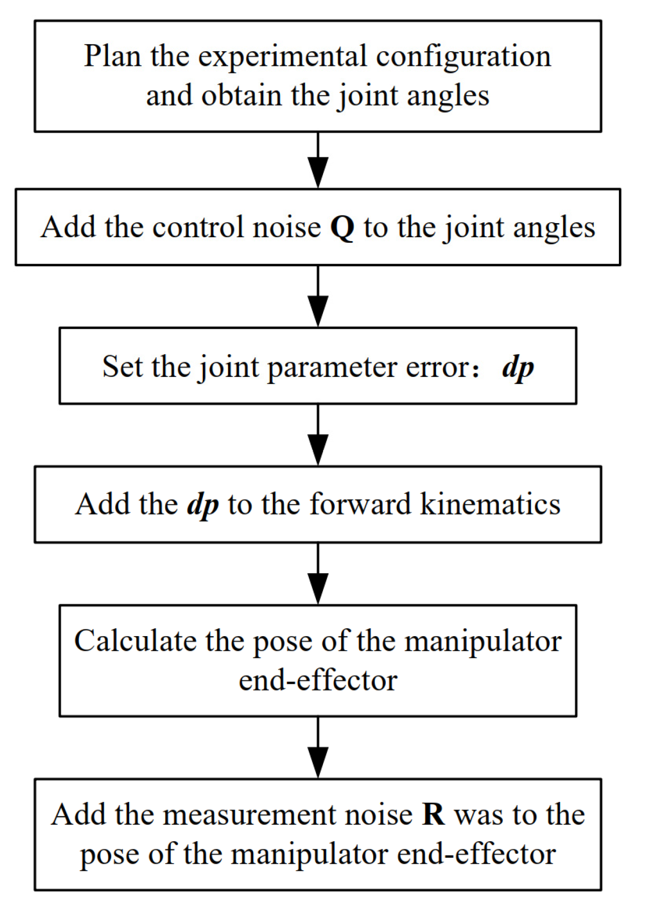
4.1. Simulation Process of a Calibration Experiment

Before conducting simulation experiments, it is necessary to build a kinematic model of the space manipulator with geometric errors. This model is capable of simulating the state of the space manipulator following launch and transfers to the space station, as is shown in Figure 4.

A predetermined set of joint parameter errors, totaling 28 parameters, is added to the kinematics model as shown in

Table 3. Error preset values of joint kinematic parameters.

Joint	$\mathit{\theta }$ (°)	$\mathit{\alpha }$ (°)	$\mathit{a}$ (mm)	$\mathit{d}$ (mm)
1	0.3	0.2	0.5	−0.9
2	−0.2	0.3	0.8	0.8
3	0.2	−0.25	−0.6	−1
4	0.3	0.3	−0.9	0.8
5	0.2	−0.3	1	0.8
6	0.2	−0.2	−0.8	0.75
7	−0.3	0.25	0.9	0.6

. Furthermore, the control noise inside the control system and the measurement noise of the end-effector should be considered. The following is the kinematic simulation before calibration.

Figure 5 depicts the entire calibration procedure of the manipulator in operation. The difference between the simulation experiment and the actual calibration of the space manipulator is that the pose error of the actual calibration is obtained by the vision system, but is derived from the kinematic model and artificially set noise in the simulation environment.

The kinematic calibration experiment with the EKF of the manipulator is divided into four parts.

1. Data acquisition: The manipulator moves to the specified pose according to the planned configuration which is nonsingular. The manipulator photographs the fixed calibration board by eye-in-hand. The pictures of the calibration board corresponding to the experimental configuration are obtained.

2. Data processing: The pictures of the calibration board are provided for calculating the real pose of the end-effector in Cartesian space according to the Zhang Zhengyou model. Additionally, the pose error of the end-effector corresponding to the experimental configuration is obtained.

3. Joint error identification: The EKF is utilized to detect the error of the manipulator joint parameters based on the end-effector position error corresponding to the experimental configuration of the manipulator.

4. Verification: According to the identified kinematic errors, the parameters in the kinematic model are corrected to ensure the accuracy of the kinematic model. A large number of configurations are chosen to verify the effect of calibration.

In order to evaluate the impact of measurement error R and control error Q on the positioning accuracy of the end-effector, we first carried out the kinematic simulation of the manipulator with two kinds of noise. Under the condition of no kinematic parameter error, the measurement error and control error are added, respectively to calculate the error of the end pose of the manipulator. With reference to [42] and combined with the design index of the space manipulator, the control noise Q and the measurement noise R are both Gaussian distributed. The average value of Q is set as 0 with the standard deviation of 0.01°. The average value of the position measurement noise is set as 0 with the standard deviation of 0.3 mm. The average value of the orientation measurement noise is set to 0 with the standard deviation of 0.5°. Figure 6 shows the pose errors of 50 groups of simulations after Q and R were added into the forward kinematics, respectively.

In EKF, the covariance matrix of the estimated state vector is a 28-dimensional diagonal matrix, which is composed of the estimation deviation of 28 kinematic parameters, an estimated angle deviation of 0.01°, and an estimated position deviation of 0.01 mm. The covariance matrix of the system prediction state is a six-dimensional diagonal matrix, which is composed of six-dimensional pose measurement noise.

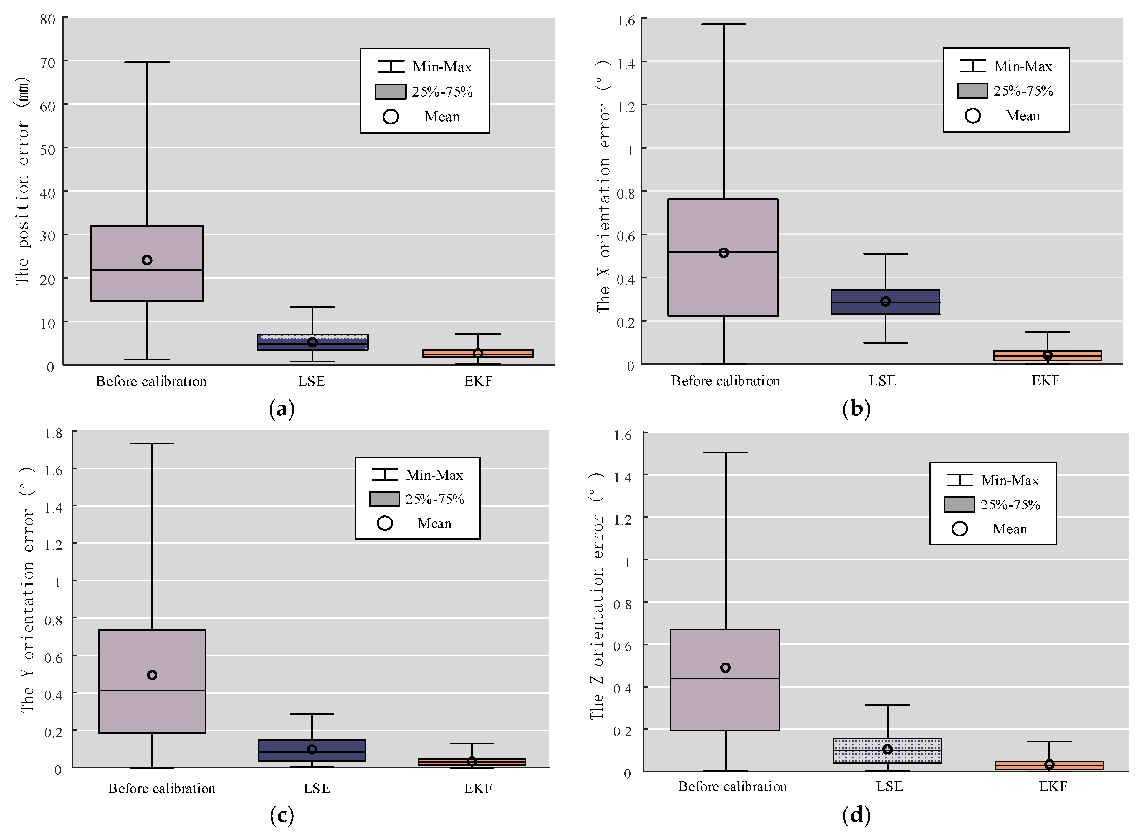
4.2. Contrast Test of Calibration Effect

The identification set consisted of 50 nonsingular configurations, and the validation set consisted of 200 nonsingular configurations. The LSE [18] and EKF are individually calibrated in order to compare pose errors before and after calibration.

Figure 7a illustrates the position accuracy of the end-effector before and after calibration. Figure 7b–d illustrate the orientation accuracy.

Table 4. Optimization effect of the position error of the calibration experiment.

		Initial	LSE		EKF
		Value	Value	Optimization Ratio	Value	Optimization Ratio
Position (mm)	Extreme values	69.9453	12.7133	81.8240%	7.3965	89.4253%
	Average value	24.2930	5.2593	78.3506%	2.3335	90.3944%
X axis orientation (°)	Extreme values	1.5867	0.5163	67.4608%	0.1473	90.7166%
	Average value	0.5188	0.2836	45.3354%	0.0467	90.9985%
Y axis orientation (°)	Extreme values	1.7236	0.2933	82.9833%	0.1432	91.6918%
	Average value	0.4951	0.1082	78.1458%	0.0237	95.2131%
Z axis orientation (°)	Extreme values	1.5012	0.3266	78.2441%	0.1147	92.3594%
	Average value	0.4802	0.1345	71.9908%	0.0335	93.0237%

Note: Optimization ratio = (initial value − EKF value)/initial value.

displays the data comparison of the pose error of the manipulator before and after calibration. Among these, the optimization ratio represents the degree of improvement of the pose accuracy.

The height of the 25–75% data box in the box plot is called the interquartile range (IQR), which can reflect the degree of data concentration. The more concentrated the data are, the lower the height of the data box is. The IQR of the EKF calibration is less than the IQR of the LSE findings, as shown in Figure 7. This indicates that the distribution of the pose errors is more concentrated after EKF calibration. Additionally, the IQR of the EKF-calibrated manipulator is lower than the LSE-calibrated manipulator. This indicates that the EKF has better calibration in terms of both position and orientation. Compared to the LSE, the EKF results fluctuate less and the calibration result is more consistent. According to Table 4, the calibration effect of the LSE for position and orientation correction varies substantially. The optimization ratio of the X axis orientation is lower by approximately 10% than the Y axis orientation and the Z axis orientation. The EKF optimization ratio of the position and orientation is almost 90%, and the performance of accuracy improvement after calibration is extremely visible. The EKF calibration effect is not only superior to the LSE in terms of total data, but it also has a stable optimization effect in terms of position and orientation.

4.3. Comparative Test of Calibration Efficiency

The researcher was aiming for an efficient calibrating method. The efficient method means that a few experimental configurations are required and high accuracy of the calibrated manipulator end-effector. In order to investigate the effect of the number of experimental configurations, simulation experiments with different numbers of experimental configurations are carried out between LSE [18] calibration and EKF calibration.

The number of experimental configurations gradually increased from 10 to 200. In each step, ten sets of experiments were carried out. The position error average of 10 sets of calibration experiments was utilized to generate a figure.

As the number of experimental configurations rises, the calibration results of both methods could be visualized in Figure 8. As a whole, EKF achieves faster convergence and requires fewer experimental configurations than LSE. When 40 sets of configurations are designed in the experiment, the EKF calibration achieved the optimal calibration effect. After 40 sets, the calibrating effect of LSE begins to diminish. With the increase in experimental configuration, the position accuracy of the end-effector improves very slowly. Increasing the number of experimental configurations has no substantial influence on the LSE identification effect after a certain point.

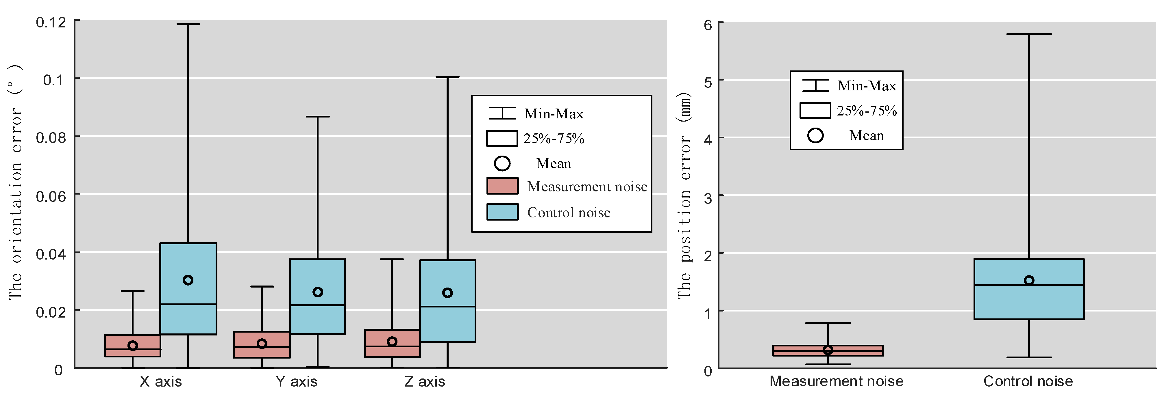
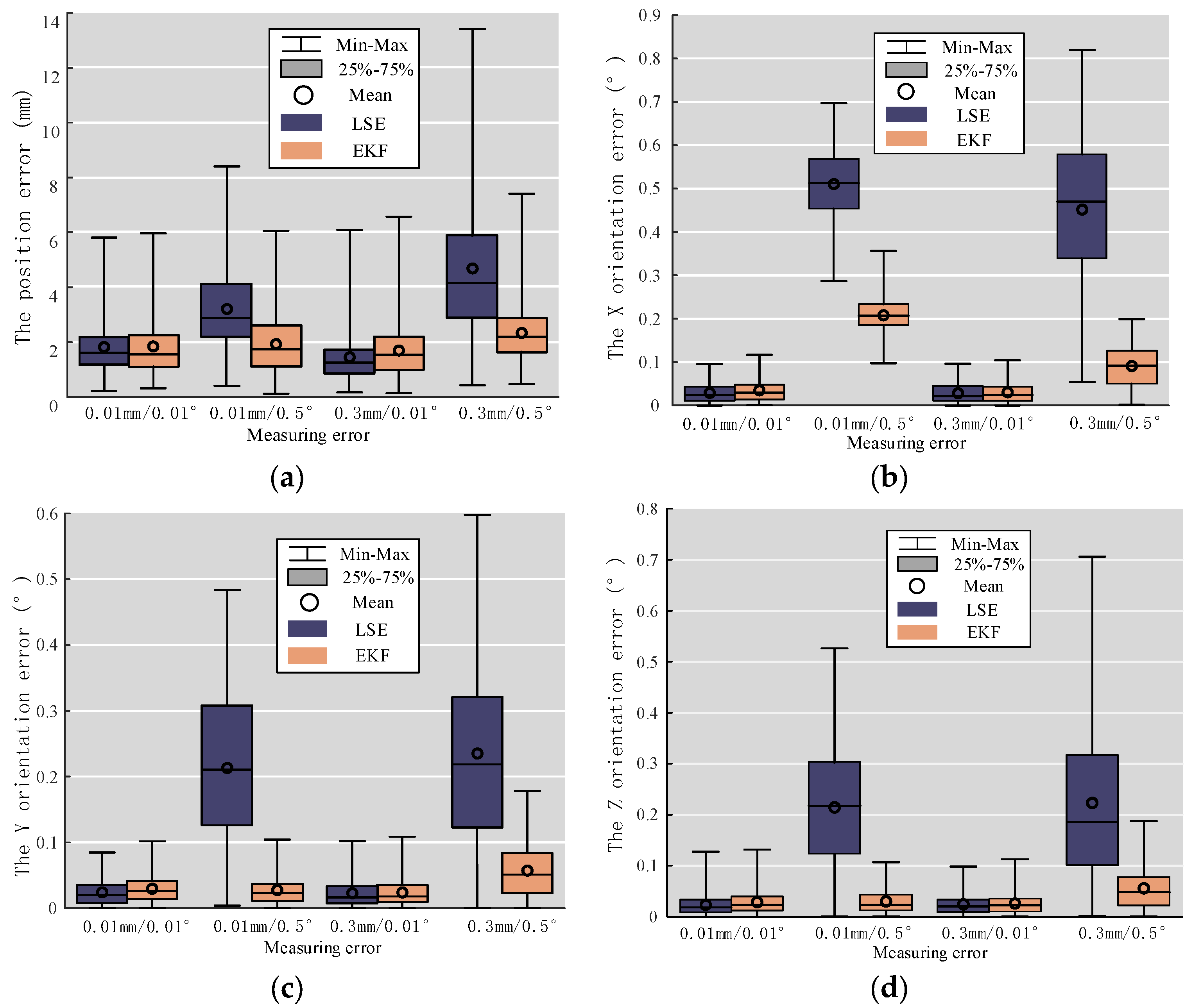
4.4. Comparative Experiment of Different Noise

In the calibration of industrial manipulators, the LSE and maximum likelihood estimation (MLE) techniques are quite common. Since space robotic arms are required to be calibrated in a short period, the MLE technique which requires a huge amount of experimental data cannot be used. Measuring equipment with high accuracy, such as laser trackers, play a vital role in LSE. However, space robotic arms lack measuring equipment with high accuracy.

We designed the simulation experiments with LSE [18] and EKF to analyze the effect of measurement noise in space. Using two distinct calibration methods, the outcomes of the manipulator which is calibrated in a cosmic environment are simulated. The measurement error in the pose of the manipulator is composed of a position error and angle error. The measurement error is divided into four categories in the simulation experiment: 0.01 mm/0.01°, 0.01 mm/0.5°, 0.3 mm/0.01°, and 0.3 mm/0.5°. Fifty configurations are utilized as experimental configurations and two hundred configurations are utilized as validation configurations.

Figure 9 depicts the box plots of the pose errors after the manipulator has been calibrated by two different methods.

Table 5. The position error after calibration.

	0.01 mm/0.01°		0.01 mm/0.5°		0.3 mm/0.01°		0.3 mm/0.5°
	Average	Extremum	Average	Extremum	Average	Extremum	Average	Extremum
LSE (mm)	1.9356	5.8736	3.1832	8.3625	1.4362	6.0831	4.7239	13.5341
EKF (mm)	1.9463	5.9541	1.9687	6.0528	1.8125	6.6727	2.4368	7.3659

displays a comparison of data for calibration results. When the measurement error is 0.01 mm/0.01°, there is no significant difference between the LSE and EKF calibration. However, when the measurement error is close to the actual measurement level of 0.3 mm/0.5° of the space manipulator, the average of the position error after calibrating by the EKF method is 2.4368 mm, and that by the LSE is 4.7239 mm. It indicates that the accuracy of the end-effector calibrated by the EKF method is higher than that by the LSE method in space. The IQR of the LSE method is higher than twice that of the EKF method. This means that the EKF calibration is more stable than LSE calibration, and that the LSE method is extremely sensitive to measurement noise. Therefore, it requires measurement equipment with high accuracy for the manipulator in practical applications. The EKF calibration method could be utilized to calibrate the manipulator with high accuracy despite high-measurement noise. It is more appropriate for calibration tasks with limited measurement accuracy, such as the kinematic calibration of the manipulator in space.

The experimental results of 0.01 mm/0.01°, 0.01 mm/0.5°, and 0.3 mm/0.01° measurement errors depicted in Figure 9 demonstrate that orientation measurement errors have a greater detrimental influence on the LSE calibration than position measurement errors. This demonstrates that the conventional LSE calibration method is more sensitive to the orientation measurement error than position measurement error.

5. Discussion

Previous research has demonstrated that the LSE is one of the most conventional and successful accessible calibration techniques. So, on the simulation platform of the space manipulator, the EKF calibration is contrasted with the LSE calibration method in this work.

The effect of the EKF is better than that of the LSE by approximately 10% in the simulation calibration of the space manipulator. The raw data and measurement noise in the simulation experiments come from the experimental data of the China Space Station.

The experimental configurations can improve the accuracy of LSE calibration and EKF calibration. However, no matter how many experimental configurations are set, the calibration effect of LSE cannot surpass that of EKF due to measurement noise

When measurement equipment with high precision is available, the difference in calibration effect between LSE and EKF is not obvious. As the measurement noise increases, the calibration effect of LSE gradually decreases, while the calibration effect of EKF has no obvious change. Therefore, the EKF has significant application relevance for calibration work with low measurement accuracy, such as a space manipulator calibration task.

Even if the measurement noise is constant, the results may fluctuate slightly when the test is repeated. This variation is mostly impacted by measuring noise and experimental configurations. A larger measuring noise and fewer experimental configurations will cause the volatility of the repeat test results to become larger. Moreover, the observability index of experimental configurations affects the result of LSE. Therefore, when an industrial manipulator is calibrated utilizing LSE, it is commonly required to screen experimental configurations with the observability index beforehand [43]. However, there is no requirement to screen the experimental configurations before calibration using the EKF. It provides researchers with a greater degree of freedom in planning the experimental configurations.

6. Conclusions

The calibration of LSE is inefficient due to the high measurement noise of the end-effector pose data, which is measured by the vision system of the space manipulator. We propose an EKF calibration approach combined with the vision measurement system in this paper. The EKF calibration method has been contrasted with the LSE calibration method based on the space manipulator simulation platform. The results revealed that the LSE calibration method is very sensitive to measurement errors and does not apply to the space manipulator. The EKF is less sensitive to measurement errors than the LSE. On the simulation platform, the optimization percentage of EKF for positioning accuracy is up to 90%, which is generally approximately 10% higher than the results of the LSE. In the box plot, the IQR of the EKF is generally less than half that of the LSE, indicating that the EKF is more stable. Furthermore, the effect of EKF calibration is unaffected by the experimental configuration, allowing for greater freedom in the design and selection of experimental configurations. Consequently, studies show that the proposed method has high accuracy, convenience, and high efficiency, and is more suited to complicated and diversified labor demands. Therefore, EKF combined with a vision measurement system is a significantly valuable application for the space manipulator.

In the measuring conditions of the space manipulator, the EKF calibration has the potential for improvement. The traditional DH method is utilized for modeling in the space manipulator control software. However, the POE method and CPC method are better suited for the calibration work than the DH modeling method. In the future, the calibration accuracy can be enhanced by converting the DH model into the POE model or CPC model.

References

1. Ma, B.; Xie, Z.; Jiang, Z.; Liu, H. Precise Semi-Analytical Inverse Kinematic Solution for 7-DOF Offset Manipulator with Arm Angle Optimization. Front. Mech. Eng. 2021, 16, 435–450. [Google Scholar] [CrossRef]
2. Liu, H.; Jiang, Z.; Liu, Y. Review of Space Manipulator Technology. Manned Spacefl. 2015, 21, 435–443. [Google Scholar] [CrossRef]
3. Meng, G.; Han, L.; Zhang, C. Research progress and technical challenges of space robot. Acta Aeronaut. Et Astronaut. Sin. 2021, 42, 8–32. [Google Scholar]
4. Liu, H.; Liu, Y.; Jiang, L. Space Robot and Teleoperation; Harbin Institute of Technology Press: Harbin, China, 2012; ISBN 978-7-5603-3806-4. (In Chinese) [Google Scholar]
5. Chen, G.; Li, T.; Chu, M.; Xuan, J.-Q.; Xu, S.-H. Review on Kinematics Calibration Technology of Serial Robots. Int. J. Precis. Eng. Manuf. 2014, 15, 1759–1774. [Google Scholar] [CrossRef]
6. Schröer, K.; Albright, S.L.; Grethlein, M. Complete, Minimal and Model-Continuous Kinematic Models for Robot Calibration. Robot. Comput. -Integr. Manuf. 1997, 13, 73–85. [Google Scholar] [CrossRef]
7. Hayati, S.A. Robot Arm Geometric Link Parameter Estimation. In Proceedings of the 22nd IEEE Conference on Decision and Control, San Antonio, TX, USA, December 1983; pp. 1477–1483. [Google Scholar] [CrossRef]
8. Veitschegger, W.K.; Wu, C.-H. Robot Calibration and Compensation. IEEE J. Robot. Automat. 1988, 4, 643–656. [Google Scholar] [CrossRef]
9. Okamura, K.; Park, F.C. Kinematic Calibration Using the Product of Exponentials Formula. Robotica 1996, 14, 415–421. [Google Scholar] [CrossRef]
10. He, R.; Zhao, Y.; Yang, S.; Yang, S. Kinematic-Parameter Identification for Serial-Robot Calibration Based on POE Formula. IEEE Trans. Robot. 2010, 26, 411–423. [Google Scholar] [CrossRef]
11. Yang, X.; Wu, L.; Li, J.; Chen, K. A Minimal Kinematic Model for Serial Robot Calibration Using POE Formula. Robot. Comput. -Integr. Manuf. 2014, 30, 326–334. [Google Scholar] [CrossRef]
12. Chen, I.-M.; Yang, G.; Tan, C.T.; Yeo, S.H. Local POE Model for Robot Kinematic Calibration. Mech. Mach. Theory 2001, 36, 1215–1239. [Google Scholar] [CrossRef]
13. Li, C.; Wu, Y.; Löwe, H.; Li, Z. POE-Based Robot Kinematic Calibration Using Axis Configuration Space and the Adjoint Error Model. IEEE Trans. Robot. 2016, 32, 1264–1279. [Google Scholar] [CrossRef]
14. Chen, G.; Wang, H.; Lin, Z. Determination of the Identifiable Parameters in Robot Calibration Based on the POE Formula. IEEE Trans. Robot. 2014, 30, 1066–1077. [Google Scholar] [CrossRef]
15. Meggiolaro, M.A.; Dubowsky, S. An Analytical Method to Eliminate the Redundant Parameters in Robot Calibration. In Proceedings of the IEEE International Conference on Robotics and Automation. Symposia Proceedings (Cat. No.00CH37065), 2000 ICRA, Millennium Conference, San Francisco, CA, USA, 24–28 April 2000; Volume 4, pp. 3609–3615. [Google Scholar] [CrossRef]
16. Gan, Y.; Duan, J.; Dai, X. A Calibration Method of Robot Kinematic Parameters by Drawstring Displacement Sensor. Int. J. Adv. Robot. Syst. 2019, 16, 172988141988307. [Google Scholar] [CrossRef]
17. Jang, J.H.; Kim, S.H.; Kwak, Y.K. Calibration of Geometric and Non-Geometric Errors of an Industrial Robot. Robotica 2001, 19, 311–321. [Google Scholar] [CrossRef] [Green Version]
18. Nubiola, A.; Bonev, I.A. Absolute Calibration of an ABB IRB 1600 Robot Using a Laser Tracker. Robot. Comput.-Integr. Manuf. 2013, 29, 236–245. [Google Scholar] [CrossRef]
19. Fachinotti, V.D.; Anca, A.A.; Cardona, A. A Method for the Solution of Certain Problems in Least Squares. Q. Appl. Math. 1944, 2, 164–168. [Google Scholar]
20. Marquardt, D.W. An Algorithm for Least-Squares Estimation of Nonlinear Parameters. J. Soc. Ind. Appl. Math. 1963, 11, 431–441. [Google Scholar] [CrossRef]
21. Zhu, Q.; Xie, X.; Li, C.; Xia, G.; Liu, Q. Kinematic Self-Calibration Method for Dual-Manipulators Based on Optical Axis Constraint. IEEE Access 2019, 7, 7768–7782. [Google Scholar] [CrossRef]
22. Du, G.; Zhang, P. Online Serial Manipulator Calibration Based on Multisensory Process via Extended Kalman and Particle Filters. IEEE Trans. Ind. Electron. 2014, 61, 6852–6859. [Google Scholar] [CrossRef]
23. Du, G.; Zhang, P.; Li, D. Online Robot Calibration Based on Hybrid Sensors Using Kalman Filters. Robot. Comput. -Integr. Manuf. 2015, 31, 91–100. [Google Scholar] [CrossRef]
24. Du, G.; Shao, H.; Chen, Y.; Zhang, P.; Liu, X. An Online Method for Serial Robot Self-Calibration with CMAC and UKF. Robot. Comput.-Integr. Manuf. 2016, 42, 39–48. [Google Scholar] [CrossRef]
25. Yang, C.; Shi, W.; Chen, W. Comparison of Unscented and Extended Kalman Filters with Application in Vehicle Navigation. J. Navig. 2017, 70, 411–431. [Google Scholar] [CrossRef]
26. Bonyan Khamseh, H.; Ghorbani, S.; Janabi-Sharifi, F. Unscented Kalman Filter State Estimation for Manipulating Unmanned Aerial Vehicles. Aerosp. Sci. Technol. 2019, 92, 446–463. [Google Scholar] [CrossRef]
27. Moghaddam, B.M.; Chhabra, R. On the Guidance, Navigation and Control of in-Orbit Space Robotic Missions: A Survey and Prospective Vision. Acta Astronaut. 2021, 184, 70–100. [Google Scholar] [CrossRef]
28. Zheng, Z.; Shirong, L.; Botao, Z. An Improved Sage-Husa Adaptive Filtering Algorithm. In Proceedings of the 31st Chinese Control Conference, Hefei, China, 25–27 July 2012; pp. 5113–5117. [Google Scholar]
29. Song, K.; Cong, S.; Deng, K.; Shang, W.; Kong, D.; Shen, H. Design of Adaptive Strong Tracking and Robust Kalman Filter. In Proceedings of the 33rd Chinese Control Conference, Nanjing, China, 28–30 July 2014; pp. 6626–6631. [Google Scholar] [CrossRef]
30. Ma, L.; Bazzoli, P.; Sammons, P.M.; Landers, R.G.; Bristow, D.A. Modeling and Calibration of High-Order Joint-Dependent Kinematic Errors for Industrial Robots. Robot. Comput.-Integr. Manuf. 2018, 50, 153–167. [Google Scholar] [CrossRef]
31. Sun, T.; Lian, B.; Zhang, J.; Song, Y. Kinematic Calibration of a 2-DoF Over-Constrained Parallel Mechanism Using Real Inverse Kinematics. IEEE Access 2018, 6, 67752–67761. [Google Scholar] [CrossRef]
32. Alıcı, G.; Jagielski, R.; Ahmet Şekercioğlu, Y.; Shirinzadeh, B. Prediction of Geometric Errors of Robot Manipulators with Particle Swarm Optimisation Method. Robot. Auton. Syst. 2006, 54, 956–966. [Google Scholar] [CrossRef]
33. Fang, L.; Dang, P. A Step Identification Method of Joint Parameters of Robots Based on the Measured Pose of End-Effector. Proc. Inst. Mech. Eng. Part C J. Mech. Eng. Sci. 2015, 229, 3218–3233. [Google Scholar] [CrossRef]
34. Cao, H.Q.; Nguyen, H.X.; Tran, T.N.-C.; Tran, H.N.; Jeon, J.W. A Robot Calibration Method Using a Neural Network Based on a Butterfly and Flower Pollination Algorithm. IEEE Trans. Ind. Electron. 2022, 69, 3865–3875. [Google Scholar] [CrossRef]
35. Wang, Z.; Chen, Z.; Mao, C.; Zhang, X. An ANN-Based Precision Compensation Method for Industrial Manipulators via Optimization of Point Selection. Math. Probl. Eng. 2020, 2020, 1–13. [Google Scholar] [CrossRef]
36. Jing, W.; Tao, P.Y.; Yang, G.; Shimada, K. Calibration of Industry Robots with Consideration of Loading Effects Using Product-Of-Exponential (POE) and Gaussian Process (GP). In Proceedings of the 2016 IEEE International Conference on Robotics and Automation (ICRA), Stockholm, Sweden, 16–21 May 2016; pp. 4380–4385. [Google Scholar] [CrossRef]
37. Shi, S.; Wang, D.; Ruan, S.; Li, R.; Jin, M.; Liu, H. High Integrated Modular Joint for Chinese Space Station Experiment Module Manipulator. In Proceedings of the 2015 IEEE International Conference on Advanced Intelligent Mechatronics (AIM), Busan, Republic of Korea, 7–11 July 2015; pp. 1195–1200. [Google Scholar] [CrossRef]
38. Ma, B.; Jiang, Z.; Liu, Y.; Xie, Z. Advances in Space Robots for On-Orbit Servicing: A Comprehensive Review. Adv. Intell. Syst. 2023. [Google Scholar]
39. Zhang, Z. A Flexible New Technique for Camera Calibration. IEEE Trans. Pattern Anal. Mach. Intell. 2000, 22, 1330–1334. [Google Scholar] [CrossRef] [Green Version]
40. Zhang, Z. Flexible Camera Calibration by Viewing a Plane from Unknown Orientations. In Proceedings of the Seventh IEEE International Conference on Computer Vision, Kerkyra, Greece, 20–27 September 1999; Volume 1, pp. 666–673. [Google Scholar] [CrossRef]
41. Huang, X.; Wang, Y. Kalman Filtering Principle and Application MATLAB Simulation; Publishing House of Electronics Industry: Beijing, China, 2015; ISBN 978-7-121-26310-1. (In Chinese) [Google Scholar]
42. Wang, G.; Shi, Z.; Shang, Y.; Sun, X.; Zhang, W.; Yu, Q. Precise Monocular Vision-Based Pose Measurement System for Lunar Surface Sampling Manipulator. Sci. China Technol. Sci. 2019, 62, 1783–1794. [Google Scholar] [CrossRef]
43. Joubair, A.; Bonev, I.A. Comparison of the Efficiency of Five Observability Indices for Robot Calibration. Mech. Mach. Theory 2013, 70, 254–265. [Google Scholar] [CrossRef]
Figure 1. The coordinate system of the space manipulator.
Machines 11 00409 g001
Figure 2. Calibration board.
Machines 11 00409 g002
Figure 3. Position of the camera in the manipulator.
Machines 11 00409 g003
Figure 4. Kinematic simulation of the manipulator before calibration.
Machines 11 00409 g004
Figure 5. Identification process.
Machines 11 00409 g005
Figure 6. Kinematics simulation of measurement noise and control noise.
Machines 11 00409 g006
Figure 7. Comparison of the recognition effect of LSE and EKF. (a) Change in the position error; (b) Change in the X axis orientation error; (c) Change in the Y axis orientation error; and (d) Change in the Z axis orientation error.
Machines 11 00409 g007
Figure 8. Calibration effect with different numbers of experimental configurations. (a) change in the position error; and (b) change in the standard deviation.
Machines 11 00409 g008
Figure 9. Calibration results with different measurement errors: (a) the position error; (b) the X orientation error; (c) the Y orientation error; and (d) the Z orientation error.
Machines 11 00409 g009