
Calculation of the Heat Flux from a Ball Screw Nut to the Nut Raceway


1
Department of Mechanical Engineering, National Chung Cheng University, Chiayi 621, Taiwan
2
Department of Energy and Refrigerating Air-Conditioning Engineering, National Taipei University of Technology, Taipei 106, Taiwan
3
HIWIN Technologies Corp., Taichung 408, Taiwan
4
Department of Mechanical Engineering and Advanced Institute of Manufacturing with High-Tech Innovations, National Chung Cheng University, Chiayi 621, Taiwan
*
Author to whom correspondence should be addressed.
Machines 2023, 11(3), 408; https://doi.org/10.3390/machines11030408
Submission received: 11 February 2023
/
Revised: 16 March 2023
/
Accepted: 20 March 2023
/
Published: 21 March 2023
(This article belongs to the Section Advanced Manufacturing)
Abstract
:In the field of precision machining, temperature fluctuation tends to cause the most significant machining errors. In particular, heat, which is generated in the nut of the ball screw feed system during movement, can deform the screw shaft significantly. In order to calculate and evaluate the thermal deformation of the ball screw shaft, the rate of the heat transfer from the nut to the screw shaft must be known. This rate can be calculated by subtracting the heat transfer rate to the nut raceway from the heat generation rate of the nut. Hence, it is necessary to calculate the heat flux from the nut to the nut raceway. This paper introduces a novel method to calculate the heat flux from the nut to the nut raceway. The new approach also enables calculations for different operating conditions. Furthermore, an experimental setup is established to measure the temperature increase, from 0 to 180 s after the nut starts moving, for various operating conditions. It is then theoretically shown that the 0–180 s temperature increase/heat flux curves for the nut are “universal”, i.e., the curve remains unchanged for the different operating conditions. Subsequently, a thermal model using the finite element method (FEM) is developed to simulate the nut temperature increase over time, which is then compared with the experimental data. As a result, it becomes possible to determine the heat flux from the nut to the nut raceway and calculate the 0–180 s temperature increase/heat flux curve () for the training group. Finally, the heat flux from the nut to the nut raceway is calculated for ten different operating conditions in the test group using the 0–180 s temperature increase/heat flux curve of the training group (). The corresponding temperature curves are then calculated by inputting the values of the heat fluxes into the FEM model. The highest root mean square error (RMSE) between the calculated and experimentally measured temperature increase was 0.16 °C for Test 7 (the error was 10.7%). This result indicates that the new method is valid and feasible for calculating the heat flux from a ball screw nut to the nut raceway.
1. Introduction
Thermal errors are the most significant errors in the commercial precision machining process. They generally account for 40–70% of the total error [1,2,3,4,5]. Among the various feed systems, ball screws are commonly used in many precision machines because of their high efficiency, rigidity, cost-effectiveness, and long service life [2,3,5]. However, during the operation of ball screws, the heat generated in both the bearing and the nut increases the temperature of the ball screw feed system (BSFS), which can lead to thermal deformation and substantially reduce positioning accuracy. To reduce the thermal error of the BSFS and to build improved high-speed and high-precision processing machines, it is necessary to study the heat generation and heat transfer involving the balls, nut, and screw shaft.
In 2004, Tian and He [6] studied the cooling effect of hollow ball screws and proposed the following equation to describe the heat generated in a nut:
where Q is the heat generation rate of the nut (kJ/h), n is the screw rotation velocity (rev/min), and τ describes the frictional torque of the nut (N–m).
Unfortunately, because Equation (1) does not consider the viscous heating effect of the lubricant (mainly determined by the kinematic viscosity), this can make the calculation of the heat generation rate of the nut less accurate. Therefore, some researchers [3,5,7,8,9,10,11] have used the following equation, which factors in the kinematic viscosity:
Here, is a factor related to the nut type and method of lubrication, and is the kinematic viscosity of the lubricant.
Because kinematic viscosity () is temperature dependent, it can be used to calculate the heat generation rate of the nut for different ambient temperatures. Using Equation (2), which considers kinematic viscosity (), Xu et al. [3,5,7,9] studied the cooling effect of hollow ball screws. The group found several ways to reduce thermal errors by employing different liquid cooling systems and cooling of the different BSFS components. Li et al. [10] proposed a response surface methodology (RSM)-based method to calculate the convective heat transfer coefficients (CHTCs) of BSFSs. Yang et al. [11] modeled the axial thermal deformation of a ball screw based on the heat generation and heat transfer analysis of the BSFS. In addition to calculating the heat generation rate of the nut using Equation (2), Oyanguren et al. [12] took into account the geometric arrangement between the nut and the ball (including contact angle and helix angle). The group concluded that the increased temperature in the nut thermally deformed the ball, which affected the nut’s preload range.
The studies above did not consider the nut as a moving heat source when the heat generation rate of the nut was calculated. During the real-life operation of a BSFS, the nut represents a moving heat source, which means that the heat generated in the nut is not transferred to a fixed position on the ball screw. Some studies have already treated the nut as a moving heat source when calculating the heat generation rate of the nut [13,14,15]. Jedrzejewski et al. [13] simulated the thermal behavior of a BSFS in a lathe. Their model considered the heat generated in the nut over time, and they calculated the temperature distribution and thermal deformation of BSFS. Li et al. [14] and Liu et al. [15] also regarded the nut as a moving heat source and were able to calculate the temperature as well as the thermal deformation at different places on the ball screw.
After determining the heat generation rate of the nut, the finite element method (FEM) [16,17,18,19,20,21,22] has been used to create a thermal model of a BSFS. Taking into account non-steady heat sources in the bearing, Horejš [16] performed a closed-loop FEM analysis for the BSFS. Their model showed a significant effect of bearing preload on the thermal stabilization of the BSFS. Li et al. [20] combined the FEM with the Monte Carlo method and proposed an adaptive real-time model (ARTM) to calculate both the temperature distribution and thermal deformation in ball screws. However, using the correct boundary conditions is particularly important for the FEM. Mao et al. [21] proposed a variable convection heat transfer coefficient model to simulate thermal stress, temperature distribution, and thermal deformation for the BSFS. This approach made it possible to set more realistic boundary conditions. Liu et al. [22] developed a hybrid response surface (HRS) thermal model for the BSFS and a multi-objective genetic algorithm (MOGA) to optimize the boundary conditions. However, even though FEM can simulate complex geometric thermal models, its mesh refinement process can be very time-consuming. Therefore, some researchers [14,15,23] derived the heat transfer equation for the BSFS using the finite difference method (FDM). In this way, they could quickly calculate the temperature distribution and thermal deformation in the BSFS for different operating conditions.
All previous studies relied on empirical equations [3,5,6,7,8,9,10,11] and considered information about the nut position [13,14,15] to calculate the heat generation rate of the nut. However, the heat generation rate of the nut alone cannot accurately describe the heat transfer processes between the balls, nut, and screw shaft. In 2018, Oyanguren et al. [12] assumed that the heat generated in the nut was equally transferred to the screw shaft and nut raceways (50% each). However, because the heat transfer processes between the balls, nut, and screw shaft during the movement of the BSFS depends on the type of movement, in this paper, a new method is proposed to determine the proportion of the generated heat transferred to the nut raceway. This makes it possible to calculate the heat flux from the nut to the nut raceway. In addition, in conjunction with the correlation equation for the frictional torque of the nut, which was proposed in our previous paper [24], the heat generation rate of the nut (q = τ × ω) can then be calculated. Furthermore, the heat transfer rate from the nut to the screw shaft can be obtained by subtracting the heat transfer rate from the nut to the nut raceways from the heat generation rate of the nut. This can be used to calculate the temperature increase as well as the thermal deformation of the screw shaft.
2. Experimental Approach
In order to calculate the heat flux from the nut to the nut raceway, an experimental setup was established that can measure the temperature in the nut (0~180 s after the nut starts moving) for different feed rates and different strokes. A schematic of the experimental setup is shown in Figure 1. The controller sends commands to the driver that drives the motor, and the coupling connects the motor with the ball screw. The length and outer diameter of the coupling, made of aluminum alloy, are 75 mm and 55 mm, respectively. The ball screw consists of balls, a nut, and a screw shaft. The screw shaft is hollow, with an outer diameter of 40 mm, an inner diameter of 12.7 mm, and a lead of 20 mm. The length and outer diameter of the nut are 143 mm and 70 mm, respectively. A flanged double nut with a preloading component is used to adjust the preload for the nut. The diameter of the balls is 6.35 mm. The balls, the nut and the screw shaft are made of carbon steel (S45C). The bearing set is composed of a pair of stainless steel NSK bearings (Model number: 30TAC62) with an outer diameter of 62 mm, an inner diameter of 30 mm and the length of 15 mm. In addition, an E-type thermocouple (5TC–TT–E–36–72, OMEGA) and a temperature acquisition card (DAQ9213, NI) were used to measure the nut temperature. The temperature measurement point was located at the bottom of the blind hole at the flange surface of the nut, and the depth of the blind hole was 15 mm. Prior to measuring the nut temperature, the thermocouple calibration experiment was conducted using a thermostatic water bath and a digital thermometer (1552A EX, FLUKE, accuracy of ±0.05 °C). In the calibration experiment, the thermocouple and digital thermometer were placed in the water bath and the temperature of the thermostatic water bath was set from 15 °C to 55 °C at 5 °C intervals for a total of 9 temperature settings (each temperature setting was left for 1 h to achieve thermal equilibrium in the thermostatic water bath). Table 1 shows the uncertainty analysis of the thermocouple calibration experiment, where the systematic error (B) is 0.1 °C for the accuracy of digital thermometer, the random errors of measurement (R) are less than 0.02 °C, and the Uncertainty (URSS) is about 0.1 °C. As shown in Table 1, the accuracy of the thermocouple reached 0.1 °C after calibration.
To study the effect of different stroke lengths, five strokes, ranging from short (50 mm) to long (900 mm), were used in the tests (900, 500, 250, 170, 90 mm). The BSFS controller had an upper limit for the rotation speed of 2000 rpm (40 m/min). The temperature change in the nut was measured for each stroke at three different feed rates (40, 20, 10 m/min). However, since the stroke lengths of 170 and 90 mm were too short, the controller’s feed rate decreased before accelerating to 40 m/min. Therefore, the 40 m/min feed rate was not considered for the 170 and 90 mm stroke lengths. Consequently, there were 13 sets of different test conditions, and the nut temperature was measured for 180 s for each scenario—see Table 2. Tests 3, 6, and 9 were used as training data to determine the nut temperature increase/heat flux curve () from 0 to 180 s for the training group—see Section 3.2 for details. Tests 1, 2, 4, 5, 7, 8, 10, 11, 12, and 13 were used as actual test data, and the corresponding heat flux from the nut to the nut raceway was calculated using the nut temperature increase/heat flux curve (0–180 s) (), which had been determined via the training group. The heat flux was used in the finite element thermal model to simulate the temperature increase in the nut. The simulated results were then compared with the measured nut temperatures to verify the validity of the new method and calculate the heat flux from the nut to the nut raceway.
3. Calculation of the Heat Flux from the Nut to the Nut Raceway
This section describes the method to calculate the heat flux from the nut to the nut raceway. In Section 3.1, it is demonstrated that the temperature increase/heat flux curve (0–180 s) for the nut is universal. Subsequently, a finite element thermal model was developed (Section 3.2) to determine the heat flux from the nut to the nut raceway. This was done by matching the experimental temperature data of the training group, which supplied the temperature increase/heat flux chart (0–180 s) of the nut (), for the training group. Finally, Section 3.3 describes how to calculate the heat flux from the nut to the nut raceway using the nut’s temperature increase/heat flux curve (0–180 s) () of the training group.
3.1. Deriving the Universality of the Temperature Increase/Heat Flux Curve (0–180 s)
Previous studies primarily focused on the heat generation in the nut and cannot accurately describe the heat transfer between the balls, the nut, and the screw shaft. This decreases the accuracy of the predicted thermal deformation of the screw shaft. In this paper, a universal equation is derived that can be used to describe the relationship between the nut temperature increase and the heat flux from the nut to the nut raceway. In this way, a more accurate calculation of the heat flux from the nut to the nut raceway becomes possible.
The equation to describe the transient heat transfer for a BSFS in a lumped–heat–capacity system is [26,27]:
where ρ is the density () of the nut, C is the specific heat (J/kg K) of the nut, V denotes the volume () of the nut, dT is temperature change (K) during time interval dt (s), h is the convective heat transfer coefficient (), A denotes the convective heat transfer surface area () of the nut, T is the nut temperature (K), is the temperature (K) of the environment, and q stands for the heat transfer rate (W) from the nut to the nut raceway. The left term in the equation represents the heat absorption rate (W) that causes the nut’s temperature to increase, and the first term on the right side of the equation reflects the heat dissipation rate (W) of the nut due to convection.
Assuming that, within the first 180 s after the nut starts to move, the heat convection boundary effect of the nut has not yet started to affect the internal temperature measurement point of the nut, then h = 0 and Equation (3) takes the form:
The variables and t can be separated readily, and for a differential time interval dt, Equation (4) can be integrated and described as follows:
Since q represents the heat transfer rate (W) from the nut to the nut raceway, and is the area of the nut raceway (0.0216 ), is defined as the heat flux () from the nut to the nut raceway. is the temperature increase curve from 0 to 180 s after the nut starts moving. In addition, since it is defined in this study that (referred to as 0–180 s temperature increase/heat flux curve in this study), Equation (5) can be transformed into Equation (6):
Equation (6) indicates that is the product of a constant and time (t), i.e., a function of time (t). Equation (6) is “universal”, which means it is valid for different operating conditions; because of that, it is the solution of Equation (3), which is an expression of the law of conservation of energy and has universality. In the next subsection, the finite element thermal model is developed, and the heat flux () from the nut to the nut raceway can be determined. The nut temperature increase (), which was measured for the training group, is then used to determine the 0–180 s temperature increase/heat flux curve () for the training group.
3.2. The Finite Element Thermal Model and Determination of the 0–180 s Temperature Increase/Heat Flux Curve
The data for the shape, size, and material of the nut and the worktable were provided by HIWIN Technologies Corporation. The numerical simulation software ANSYS® [28] was used to build the finite element thermal model of the nut and the worktable and set the model parameters (material properties, including density, specific heat, thermal conductivity, and thermal expansion coefficient). The boundary conditions were determined using the three-dimensional transient heat transfer equation and the empirical equation for thermal convection. The corresponding parameters and equations were taken from previous studies [29,30], where more technical details can be found. In this study, the heat generation rate of the nut was calculated using Equation (2) given in the Introduction section. The heat transfer mode of moving components, including the nut and worktable, belongs to forced convection. Equation (7) was used to calculate the forced convection heat transfer coefficient. Through this equation, the forced convection heat transfer coefficient near the nut and worktable can be calculated [22,29,30]:
where Nu is the Nusselt number , Re is the Reynolds number, Pr is the Prandtl number, is the thermal conductivity of the surrounding air, and L is the characteristic length.
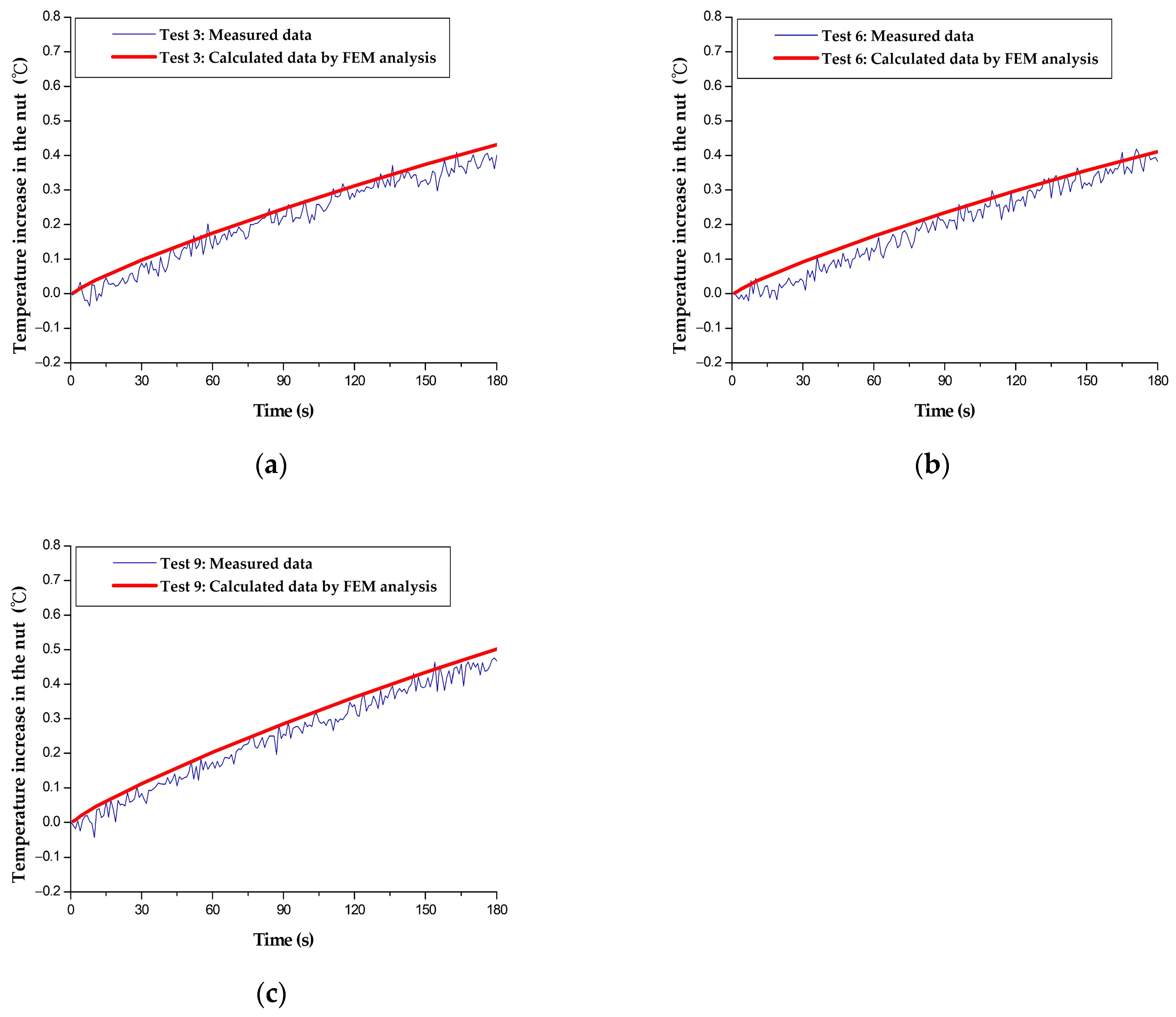
In this study, the nut temperature increase was simulated using the finite element thermal model, and the trial-and-error method was used to adjust the proportion of the heat generation rate of the nut allocated to the nut raceway. This was done to minimize the root mean square error (RMSE) between the FEM-simulated nut temperature increase and the experimental data for the training groups (Tests 3, 6, 9). The determined proportion of heat allocated to the nut raceway was then converted into the heat fluxes from the nut to the nut raceways. As shown in Figure 2, the heat fluxes from the nut to the nut raceways in Tests 3, 6, and 9 were, respectively, 355, 339, and 413 . The RMSEs between the FEM simulation results and experimental data were calculated using the following equation:
where i is the measurement index of time in seconds, is the experimentally measured nut temperature increase, and is the FEM simulated nut temperature increase. The calculated RMSEs for Tests 3, 6, and 9 were 0.03, 0.04, and 0.04 respectively, which reflects the accuracy of the heat flux from the nut to the nut raceway for the training set.
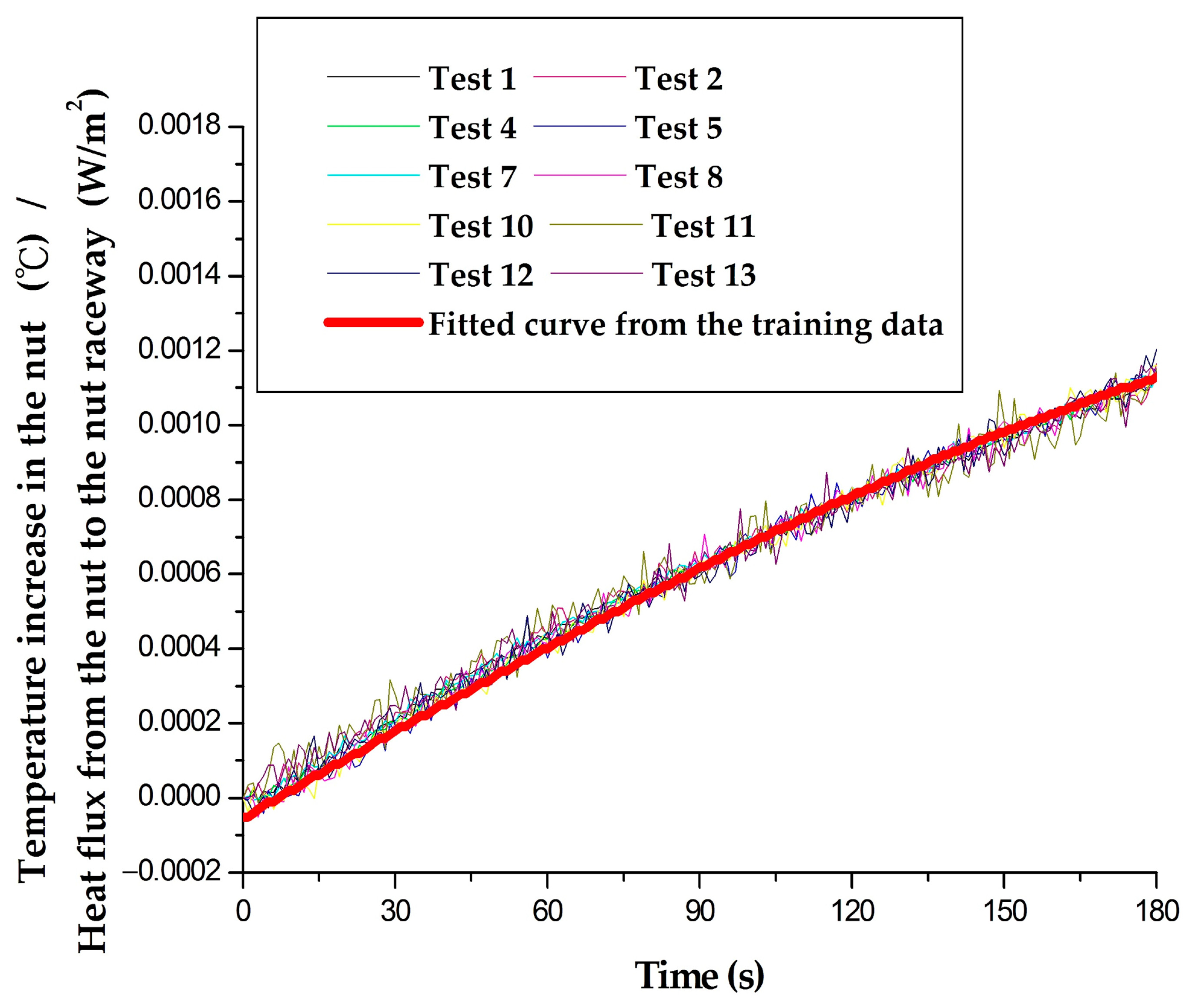
According to Equation (6), the measured nut temperature increase in the training set was divided by the heat flux from the nut to the nut raceway (determined by the FEM). The results are shown in Figure 3. The three curves for Tests 3, 6, and 9 overlap, which confirms that the nut temperature increase () is proportional to the heat flux from the nut to the nut raceway. In order to facilitate the calculation of the heat flux from the nut to the nut raceways for the test group, the three data sets obtained from the training group were fitted using one curve—see the red line in Figure 3. A third-degree polynomial can describe the fitted curve. The coefficients are, respectively, , , , and , and the coefficient of determination . In this study, the fitted curve is referred to as the 0–180 s temperature increase/heat flux curve () for the training group. Because the 0–180 s temperature increase/heat flux curve remains the same under different operating conditions, the fitted curve has universal characteristics. In this study, this curve will be used for different operating conditions to calculate the heat flux from the nut to the nut raceway.
3.3. Calculation of the Heat Flux from the Nut to the Nut Raceway Using the 0–180 s Temperature Increase/Heat Flux Curve
To calculate the heat flux from the nut to the nut raceway of the test group, with reference to the form of Equation (6), the measured nut temperature curves () of the test group were divided by different heat flux values. This yields the curve (curve 1). The 0–180 s temperature increase/heat flux curve (), which was obtained in the previous subsection for the training group, is referred to as curve 2. The heat flux, associated with the minimum sum of squared errors (SSE) between curves 1 and 2, is the heat flux from the nut to the nut raceway for the corresponding operating condition.
The finite element thermal model typically requires continuous adjustment of the heat transfer rate via trial and error to simulate the nut temperature increase. The simulation results are then compared with experimental data to determine the heat flux rate from the nut to the nut raceway. This process is very time consuming and labor intensive. However, thanks to the universality of the 0–180 s temperature increase/heat flux curve, the 0–180 s temperature increase/heat flux curve could be obtained for the training group () using a small amount of nut temperature data and the finite element thermal model. This then allowed the quick determination of the heat flux from the nut to the nut raceway for other operating conditions, which saves computation time for the finite element thermal model.
4. Results and Discussion
According to Section 3.3, the heat flux from the nut to the nut raceway for the ten operating conditions in the test group can be calculated by minimizing the SSE between the two curves. The results are shown in Table 3. The temperature increase/heat flux curves for the nut were obtained by dividing the experimental nut temperature curves by the heat flux determined for the ten operating conditions—see Figure 4. The figure shows that the curves for the ten operating conditions are very similar to the curves of the training group (, red line in Figure 4). This confirms that the 0–180 s temperature increase/heat flux curve derived in Section 3.1 is, in fact, universal.
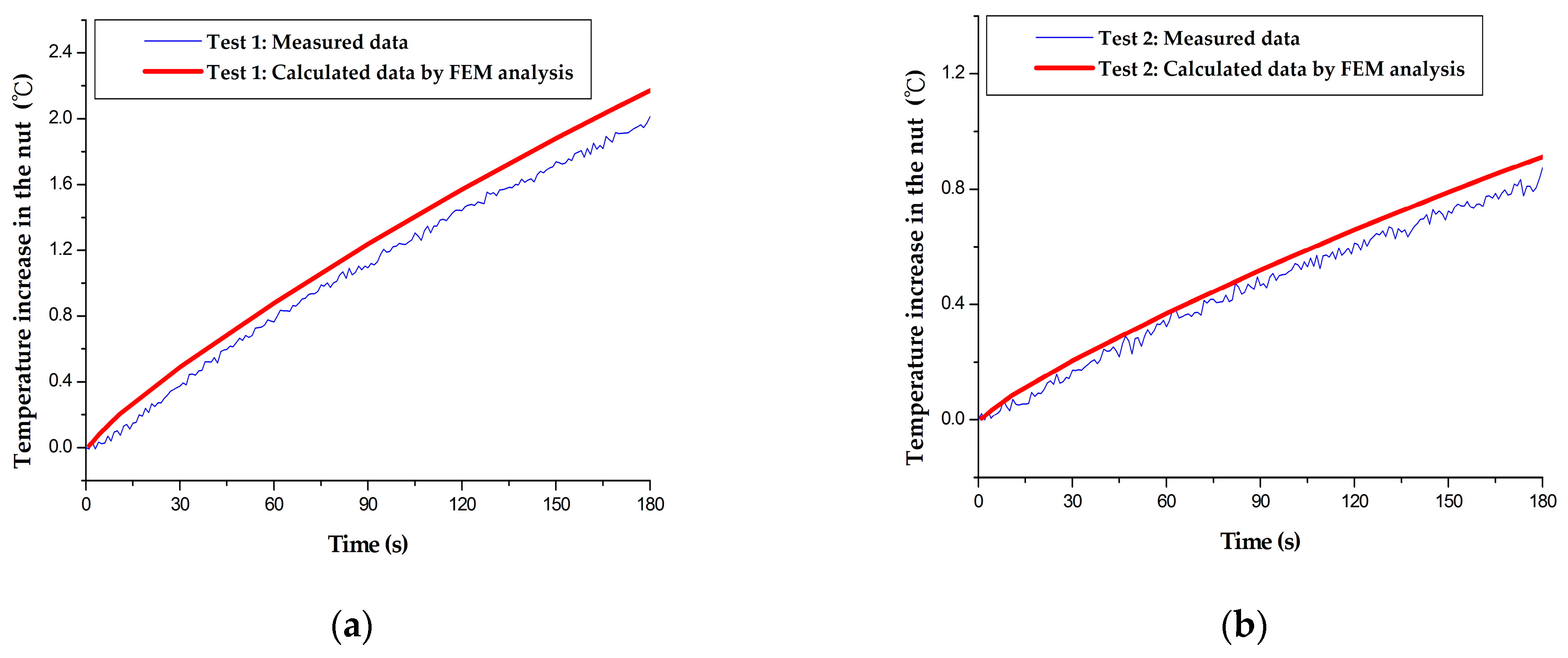
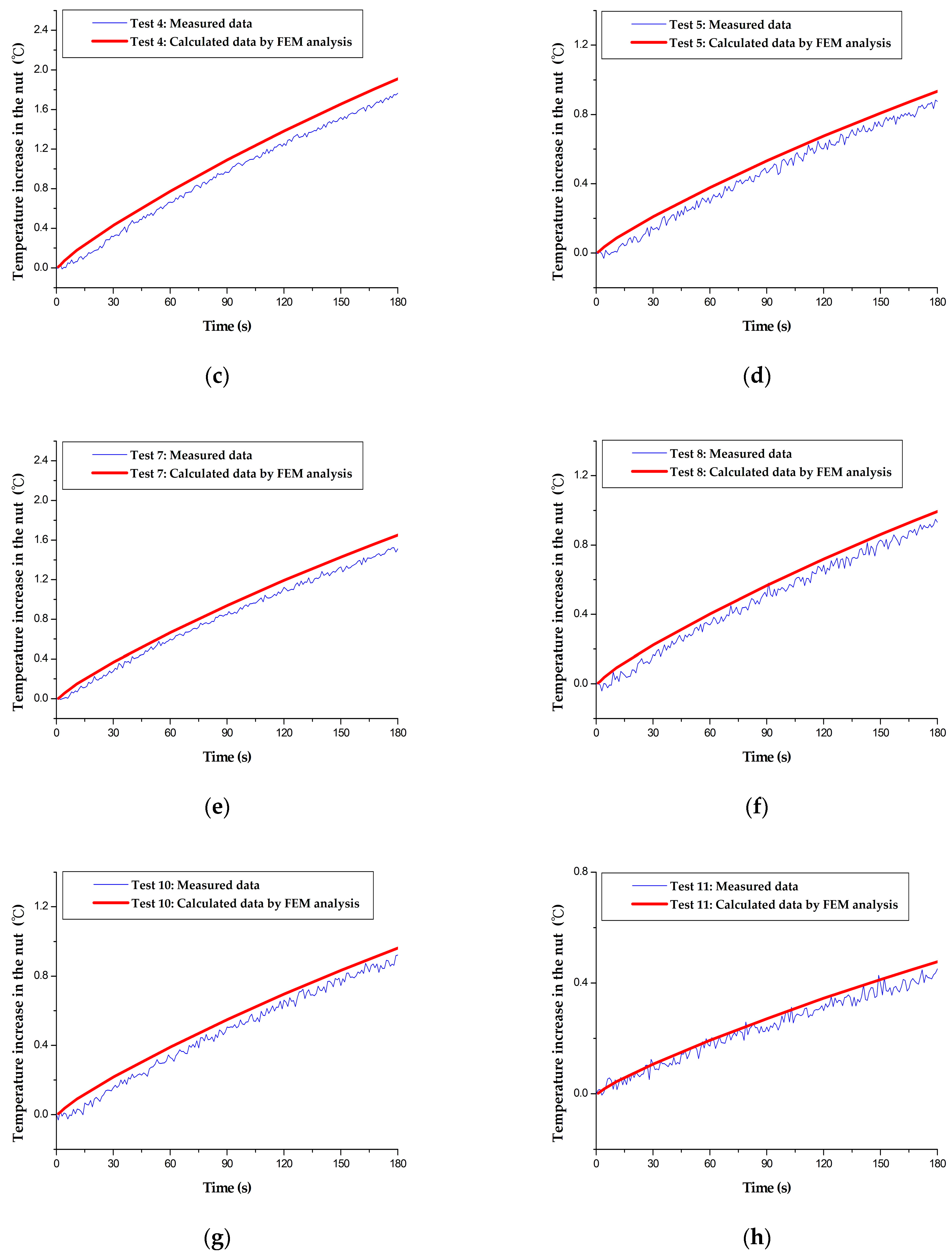
In order to validate the proposed method, the heat flux values of the test group were used as inputs for the finite element thermal model. This made it possible to simulate the nut temperature increase curves, which were then compared with the measured results (Figure 5). The RMSE results are listed in Table 3. The maximum RMSE was 0.16 °C for Test 7, and the corresponding measured temperature increase of the nut was 1.51 °C for 180 s; thus, the error was 10.7%. Because the simulated temperature increase of the nut (using the finite element thermal model) is very close to the measured data, it can be concluded that the new method works sufficiently accurately.
5. Summary and Conclusions
In this study, a new method was proposed to calculate the heat flux from a ball screw nut to the nut raceway. First, a finite element thermal model was developed to determine the heat flux for three tests in a training group using trial and error. The respective values were 355, 339, and 413 . The measured temperature increase curves for the nut of the training group were then divided by the corresponding heat flux, and the resultant curves were fitted to obtain a 0–180 s temperature increase/heat flux curve of the training group (). The high coefficient of determination, , indicated good fitting of the curve. Subsequently, the measured curves () of the test group were divided by different heat fluxes to yield the curve . By minimizing the SSE between the two curves ( and ), the heat flux could then be determined for the ten operating conditions in the test group. These heat flux values were used as inputs for the finite element thermal model to simulate the nut temperature curves, which were then compared with the measured results. The maximum RMSE was 0.16 °C (error = 10.7%) for Test 7. This indicates that the simulated and measured temperature increase in the nut was very similar and confirms the validity of the new method.
The effective simulation of the nut temperature increase via the finite element thermal model typically required continuous adjustment of the heat transfer rate using trial and error. Using the new method, this very time consuming and labor intensive process could be simplified thanks to the general validity of the 0–180 s temperature increase/heat flux curve. With its help, the 0–180 s temperature increase/heat flux curve could be obtained for the training group (), requiring only a small amount of nut temperature data. In other words, it is now possible to quickly determine the heat flux from the nut to the nut raceway for various operating conditions. This saves substantial computation time for the finite element thermal model.
In addition, both the preload of the nut and pretension of the screw shaft change with increasing usage time of the BSFS and the type of method used. The new method enables the fast calculation of the heat flux from a ball screw nut to the nut raceways and the real time prediction of the heat-caused deformation of the screw, which is crucial to improve positioning accuracy.
Author Contributions
Conceptualization, T.-C.K., A.-S.Y., Y.-C.H. and W.-H.H.; methodology, T.-C.K., A.-S.Y., Y.-C.H. and W.-H.H.; software, T.-C.K., A.-S.Y. and W.-H.H.; validation, T.-C.K., A.-S.Y. and W.-H.H.; formal analysis, T.-C.K., A.-S.Y. and W.-H.H.; investigation, T.-C.K., A.-S.Y., Y.-C.H. and W.-H.H.; resources, A.-S.Y., Y.-C.H. and W.-H.H.; data curation, T.-C.K., A.-S.Y. and W.-H.H.; writing—original draft preparation, T.-C.K., A.-S.Y. and W.-H.H.; writing—review and editing, T.-C.K., A.-S.Y., Y.-C.H. and W.-H.H.; visualization, T.-C.K., A.-S.Y. and W.-H.H.; supervision, A.-S.Y., Y.-C.H. and W.-H.H.; project administration, A.-S.Y., Y.-C.H. and W.-H.H.; funding acquisition, A.-S.Y., Y.-C.H. and W.-H.H. All authors have read and agreed to the published version of the manuscript.
Funding
This research was funded by the Ministry of Science and Technology, Taiwan, under grant number MOST 106-2622-E-194-003-CC2.
Data Availability Statement
Not applicable.
Acknowledgments
This work was partially supported by the HIWIN Technologies Corporation.
Conflicts of Interest
The authors declare no conflict of interest.
References
- Yun, W.S.; Kim, S.K.; Cho, D.W. Thermal error analysis for a CNC lathe feed drive system. Int. J. Mach. Tools Manuf. 1999, 39, 1087–1101. [Google Scholar] [CrossRef]
- Ahn, J.; Chung, S. Real-time estimation of the temperature distribution and expansion of a ball screw system using an observer. Proc. Inst. Mech. Eng. Part B J. Eng. Manuf. 2004, 218, 1667–1681. [Google Scholar] [CrossRef]
- Xu, Z.; Liu, X.; Kim, H.; Shin, J.; Lyu, S. Thermal error forecast and performance evaluation for an air-cooling ball screw system. Int. J. Mach. Tools Manuf. 2011, 51, 605–611. [Google Scholar] [CrossRef]
- Jin, C.; Wu, B.; Hu, Y. Heat generation modeling of ball bearing based on internal load distribution. Tribol. Int. 2012, 45, 8–15. [Google Scholar] [CrossRef]
- Xu, Z.Z.; Liu, X.J.; Choi, C.H.; Lyu, S.K. A study on improvement of ball screw system positioning error with liquid–cooling. Int. J. Precis. Eng. Manuf. 2012, 13, 2173–2181. [Google Scholar] [CrossRef]
- Tian, R.; He, R. Solution for heating of ball screw and environmental engineering. World Manuf. Eng. Mark. 2004, 3, 65–67. [Google Scholar]
- Xu, Z.Z.; Liu, X.J.; Lyu, S.K. Study on positioning accuracy of nut/shaft air cooling ball screw for high-precision feed drive. Int. J. Precis. Eng. Manuf. 2014, 15, 111–116. [Google Scholar] [CrossRef]
- Shi, H.; Ma, C.; Yang, J.; Zhao, L.; Mei, X.; Gong, G. Investigation into effect of thermal expansion on thermally induced error of ball screw feed drive system of precision machine tools. Int. J. Mach. Tools Manuf. 2015, 97, 60–71. [Google Scholar] [CrossRef]
- Xu, Z.Z.; Choi, C.; Liang, L.J.; Li, D.Y.; Lyu, S.K. Study on a novel thermal error compensation system for high-precision ball screw feed drive (1st report: Model, calculation and simulation). Int. J. Precis. Eng. Manuf. 2015, 16, 2005–2011. [Google Scholar] [CrossRef]
- Li, D.; Feng, P.; Zhang, J.; Wu, Z.; Yu, D. Method for modifying convective heat transfer coefficients used in the thermal simulation of a feed drive system based on the response surface methodology. Nume. Heat Transf. A Appl. 2016, 69, 51–66. [Google Scholar] [CrossRef]
- Yang, J.; Li, C.; Xu, M.; Zhang, Y. Analysis of thermal error model of ball screw feed system based on experimental data. Int. J. Adv. Manuf. Technol. 2022, 119, 7415–7427. [Google Scholar] [CrossRef]
- Oyanguren, A.; Larranaga, J.; Ulacia, I. Thermo-mechanical modelling of ball screw preload force variation in different working conditions. Int. J. Adv. Manuf. Technol. 2018, 97, 723–739. [Google Scholar] [CrossRef]
- Jedrzejewski, J.; Kowal, Z.; Kwasny, W.; Winiarski, Z. Ball screw unit precise modelling with dynamics of loads and moving heat sources taken into account. J. Mach. Eng. 2019, 19, 27–41. [Google Scholar] [CrossRef]
- Li, Y.; Wei, W.; Su, D.; Wu, W.; Zhang, J.; Zhao, W. Thermal characteristic analysis of ball screw feed drive system based on finite difference method considering the moving heat source. Int. J. Adv. Manuf. Technol. 2020, 106, 4533–4545. [Google Scholar] [CrossRef]
- Liu, H.; Rao, Z.; Pang, R.; Zhang, Y. Research on Thermal Characteristics of Ball Screw Feed System Considering Nut Movement. Machines 2021, 9, 249. [Google Scholar] [CrossRef]
- Horejs, O. Thermo–mechanical model of ball screw with non-steady heat sources. In Proceedings of the International Conference on Thermal Issues in Emerging Technologies—Theory and Application, Cairo, Egypt, 3–6 January 2007. [Google Scholar]
- Min, X.; Jiang, S. A thermal model of a ball screw feed drive system for a machine tool. Proc. Inst. Mech. Eng. C J. Mech. Eng. Sci. 2011, 225, 186–193. [Google Scholar] [CrossRef]
- Uhlmann, E.; Hu, J. Thermal modelling of an HSC machining centre to predict thermal error of the feed system. Prod. Eng. 2012, 6, 603–610. [Google Scholar] [CrossRef]
- Yang, J.; Zhang, D.; Mei, X.; Zhao, L.; Ma, C.; Shi, H. Thermal error simulation and compensation in a jig–boring machine equipped with a dual-drive servo feed system. Proc. Inst. Mech. Eng. B J. Eng. Manuf. 2014, 229, 43–63. [Google Scholar] [CrossRef]
- Li, T.J.; Zhao, C.Y.; Zhang, Y.M. Adaptive real–time model on thermal error of ball screw feed drive systems of CNC machine tools. Int. J. Adv. Manuf. Technol. 2017, 94, 3853–3861. [Google Scholar] [CrossRef]
- Mao, X.; Mao, K.; Du, Y.; Wang, F.; Yan, B. Analysis of the Thermal Characteristics of Machine Tool Feed System Based on Finite Element Method. IOP Conf. Ser. Mater. Sci. Eng. 2017, 234, 012013. [Google Scholar] [CrossRef]
- Liu, J.; Ma, C.; Wang, S.; Wang, S.; Yang, B.; Shi, H. Thermal boundary condition optimization of ball screw feed drive system based on response surface analysis. Mech. Syst. Signal Process. 2019, 121, 471–495. [Google Scholar] [CrossRef]
- Xia, J.; Hu, Y.; Wu, B.; Shi, T. Numerical solution, simulation and testing of the thermal dynamic characteristics of ball-screws. Front. Mech. Eng. China 2008, 3, 28–36. [Google Scholar] [CrossRef]
- Kuo, T.C.; Hwang, Y.C.; Hsieh, W.H. A New Correlation Equation for Calculating the Frictional Torque of the Nut at Different Feed Velocities and Nut Temperatures. Int. J. Precis. Eng. Manuf. 2021, 22, 41–50. [Google Scholar] [CrossRef]
- Robert, P.B. Uncertainties and Statistics. In Fundamentals of Temperature, Pressure, and Flow Measurements, 3rd ed.; John Wiley & Sons Ltd.: New York, NY, USA, 1984; pp. 172–199. [Google Scholar]
- Kreith, F.; Bohn, M.S. Heat Conduction. In Principles of Heat Transfer, 5th ed.; West Publishing: Eagan, MN, USA, 1993; pp. 120–121. [Google Scholar]
- Holman, J.P. Unsteady-State Condition. In Heat Transfer, 8th ed.; McGraw-Hill: New York, NY, USA, 1997; pp. 142–143. [Google Scholar]
- ANSYS. 13 User Guide; ANSYS Inc.: Canonsburg, PA, USA, 2010. Available online: www.ansys.com (accessed on 1 February 2015).
- Yang, A.S.; Chai, S.Z.; Hsu, H.H.; Kuo, T.C.; Wu, W.T.; Hsieh, W.H.; Hwang, Y.C. FEM–based modeling to simulate thermal deformation process for high–speed ball screw drive systems. Appl. Mech. Mater. 2013, 481, 171–179. [Google Scholar] [CrossRef]
- Yang, A.S.; Chai, S.Z.; Hsu, H.H.; Kuo, T.C.; Wu, W.T.; Hsieh, W.H.; Hwang, Y.C. Prediction of thermal deformation for a ball screw system under composite operating conditions. In Transactions on Engineering Technologies; Yang, G.C., Ao, S.I., Gelman, L., Eds.; Springer: Dordrecht, The Netherlands; Berlin, Germany, 2014; pp. 17–30. [Google Scholar]
Figure 1.
Schematic diagram of the experimental setup.

Figure 2.
Comparison of the FEM-simulated and the measured nut temperatures for the training group: (a) Test 3; (b) Test 6; (c) Test 9.
Figure 2.
Comparison of the FEM-simulated and the measured nut temperatures for the training group: (a) Test 3; (b) Test 6; (c) Test 9.

Figure 3.
Experimental measurement of the nut temperature increase, divided by the FEM-simulated heat flux from the nut to the nut raceway for the training group.
Figure 3.
Experimental measurement of the nut temperature increase, divided by the FEM-simulated heat flux from the nut to the nut raceway for the training group.

Figure 4.
Experimental nut temperature increase, divided by the heat flux from the nut to the nut raceway for the test group.
Figure 4.
Experimental nut temperature increase, divided by the heat flux from the nut to the nut raceway for the test group.

Figure 5.
Comparison of the FEM-simulated and measured nut temperature curves of the test group: (a) Test 1; (b) Test 2; (c) Test 4; (d) Test 5; (e) Test 7; (f) Test 8; (g) Test 10; (h) Test 11; (i) Test 12; (j) Test 13.
Figure 5.
Comparison of the FEM-simulated and measured nut temperature curves of the test group: (a) Test 1; (b) Test 2; (c) Test 4; (d) Test 5; (e) Test 7; (f) Test 8; (g) Test 10; (h) Test 11; (i) Test 12; (j) Test 13.


Table 1.
Uncertainty analysis of the thermocouple calibration experiment.
| Average temperature (°C) | 15.054 | 20.006 | 25.007 | 29.954 | 34.992 | 40.017 | 45.031 | 49.957 | 54.963 |
| Sample standard deviation (°C) | 0.0191 | 0.0167 | 0.0173 | 0.0188 | 0.0221 | 0.0181 | 0.0239 | 0.0197 | 0.0300 |
| Systematic error (°C) | 0.1 | 0.1 | 0.1 | 0.1 | 0.1 | 0.1 | 0.1 | 0.1 | 0.1 |
| Sample standard deviation of the mean (°C) | 0.0043 | 0.0037 | 0.0039 | 0.0042 | 0.0049 | 0.0041 | 0.0053 | 0.0044 | 0.0067 |
| t value for 95% confidence (n = 20) | 2.093 | 2.093 | 2.093 | 2.093 | 2.093 | 2.093 | 2.093 | 2.093 | 2.093 |
| Random error (°C) | 0.0089 | 0.0078 | 0.0081 | 0.0088 | 0.0103 | 0.0085 | 0.0112 | 0.0092 | 0.0140 |
| Uncertainty (URSS, Probable Uncertainty, [25]) | 0.1004 | 0.1003 | 0.1003 | 0.1004 | 0.1005 | 0.1004 | 0.1006 | 0.1004 | 0.1010 |
Table 2.
Overview of the used test conditions.
| Test Conditions | 1 | 2 | 3 | 4 | 5 | 6 | 7 | 8 | 9 | 10 | 11 | 13 | 14 |
|---|---|---|---|---|---|---|---|---|---|---|---|---|---|
| Stroke length (mm) | 900 | 900 | 900 | 500 | 500 | 500 | 250 | 250 | 250 | 170 | 170 | 90 | 90 |
| Feed rate (m/min) | 40 | 20 | 10 | 40 | 20 | 10 | 40 | 20 | 10 | 20 | 10 | 20 | 10 |
| Measurement time (s) | 180 | 180 | 180 | 180 | 180 | 180 | 180 | 180 | 180 | 180 | 180 | 180 | 180 |
| Training data | V | V | V | ||||||||||
| Test data | V | V | V | V | V | V | V | V | V | V |
Table 3.
Heat flux from the nut to the nut raceway of the test group and calculated RMSE between simulated and experimental nut-temperature increase.
Table 3.
Heat flux from the nut to the nut raceway of the test group and calculated RMSE between simulated and experimental nut-temperature increase.
| Test Conditions | Test 1 | Test 2 | Test 4 | Test 5 | Test 7 |
| Moving stroke (mm) | 900 | 900 | 500 | 500 | 250 |
| Feed rate (m/min) | 40 | 20 | 40 | 20 | 40 |
| Heat flux from the nut to the nut raceway () | 1786 | 750 | 1558 | 765 | 1344 |
| RMSE (°C) | 0.12 | 0.06 | 0.09 | 0.07 | 0.16 |
| Test Conditions | Test 8 | Test 10 | Test 11 | Test 12 | Test 13 |
| Moving stroke (mm) | 250 | 170 | 170 | 90 | 90 |
| Feed rate (m/min) | 20 | 20 | 10 | 20 | 10 |
| Heat flux from the nut to the nut raceway () | 820 | 794 | 392 | 580 | 432 |
| RMSE (°C) | 0.06 | 0.06 | 0.04 | 0.06 | 0.04 |
Disclaimer/Publisher’s Note: The statements, opinions and data contained in all publications are solely those of the individual author(s) and contributor(s) and not of MDPI and/or the editor(s). MDPI and/or the editor(s) disclaim responsibility for any injury to people or property resulting from any ideas, methods, instructions or products referred to in the content. |
© 2023 by the authors. Licensee MDPI, Basel, Switzerland. This article is an open access article distributed under the terms and conditions of the Creative Commons Attribution (CC BY) license (https://creativecommons.org/licenses/by/4.0/).
Share and Cite
MDPI and ACS Style
Kuo, T.-C.; Yang, A.-S.; Hwang, Y.-C.; Hsieh, W.-H. Calculation of the Heat Flux from a Ball Screw Nut to the Nut Raceway. Machines 2023, 11, 408. https://doi.org/10.3390/machines11030408
AMA Style
Kuo T-C, Yang A-S, Hwang Y-C, Hsieh W-H. Calculation of the Heat Flux from a Ball Screw Nut to the Nut Raceway. Machines. 2023; 11(3):408. https://doi.org/10.3390/machines11030408
Chicago/Turabian StyleKuo, Tzu-Chien, An-Shik Yang, Yih-Chyun Hwang, and Wen-Hsin Hsieh. 2023. "Calculation of the Heat Flux from a Ball Screw Nut to the Nut Raceway" Machines 11, no. 3: 408. https://doi.org/10.3390/machines11030408
Note that from the first issue of 2016, this journal uses article numbers instead of page numbers. See further details here.