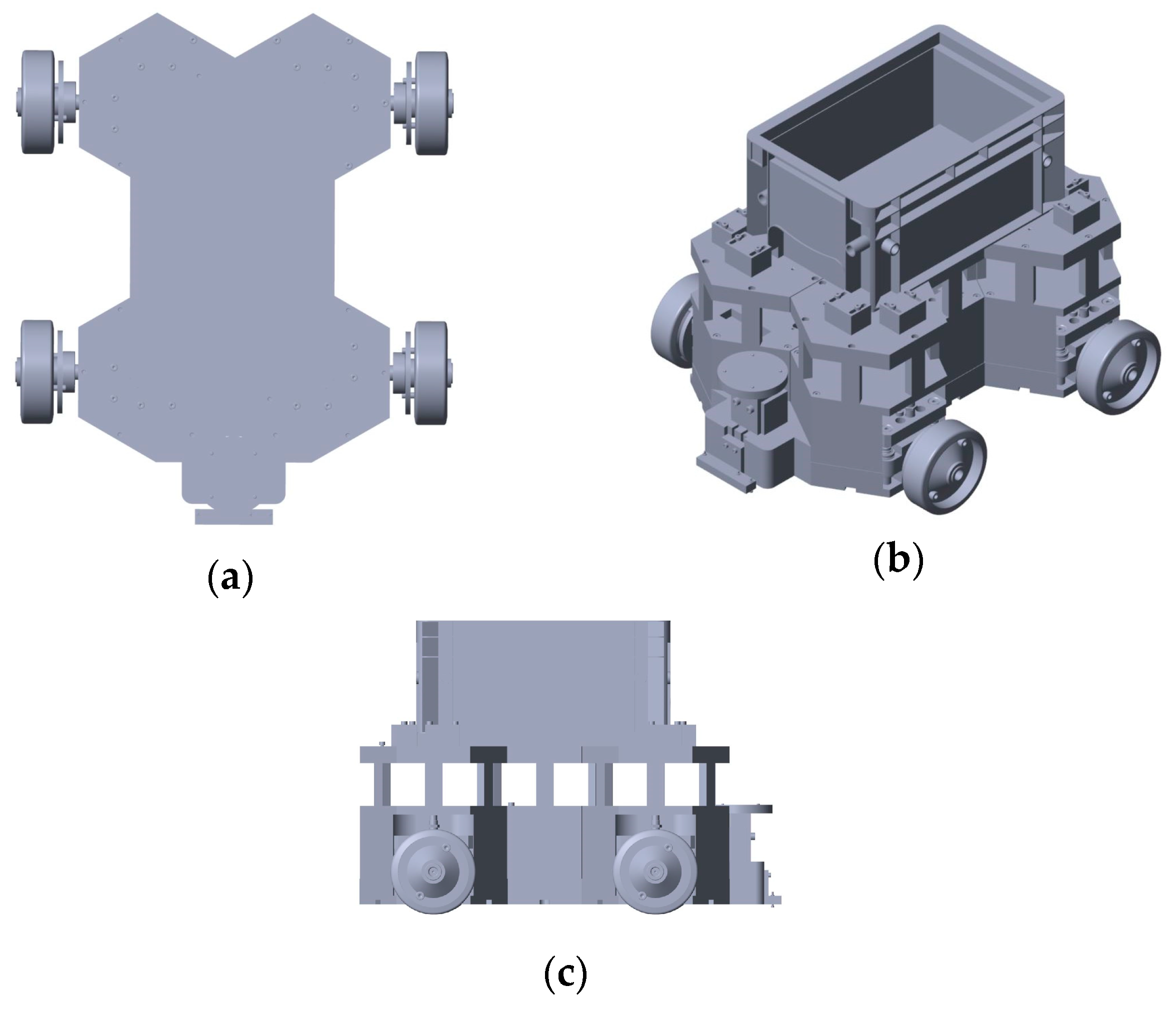
Figure 1.
Possible configurations of the modular mobile platform. (a) Mobile robot with two conventional wheels. (b) Mobile robot with three omnidirectional wheels. (c) Mobile robot with four conventional wheels.
Figure 1.
Possible configurations of the modular mobile platform. (a) Mobile robot with two conventional wheels. (b) Mobile robot with three omnidirectional wheels. (c) Mobile robot with four conventional wheels.
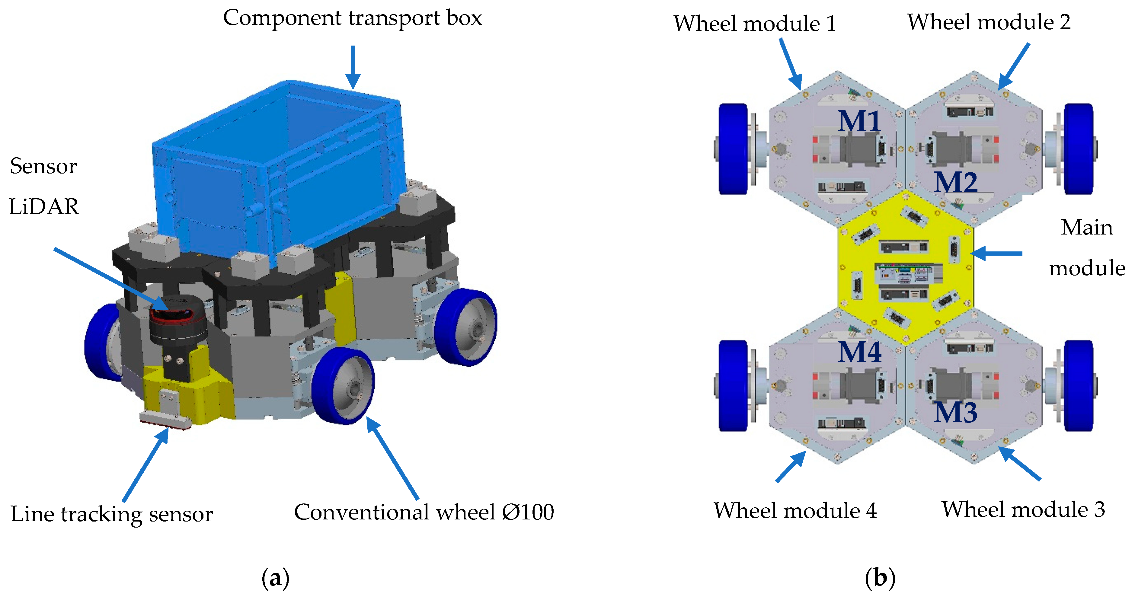
Figure 2.
Modular mobile robot with four conventional wheels (3D model). (a) Isometric view. (b) Bottom view.
Figure 2.
Modular mobile robot with four conventional wheels (3D model). (a) Isometric view. (b) Bottom view.
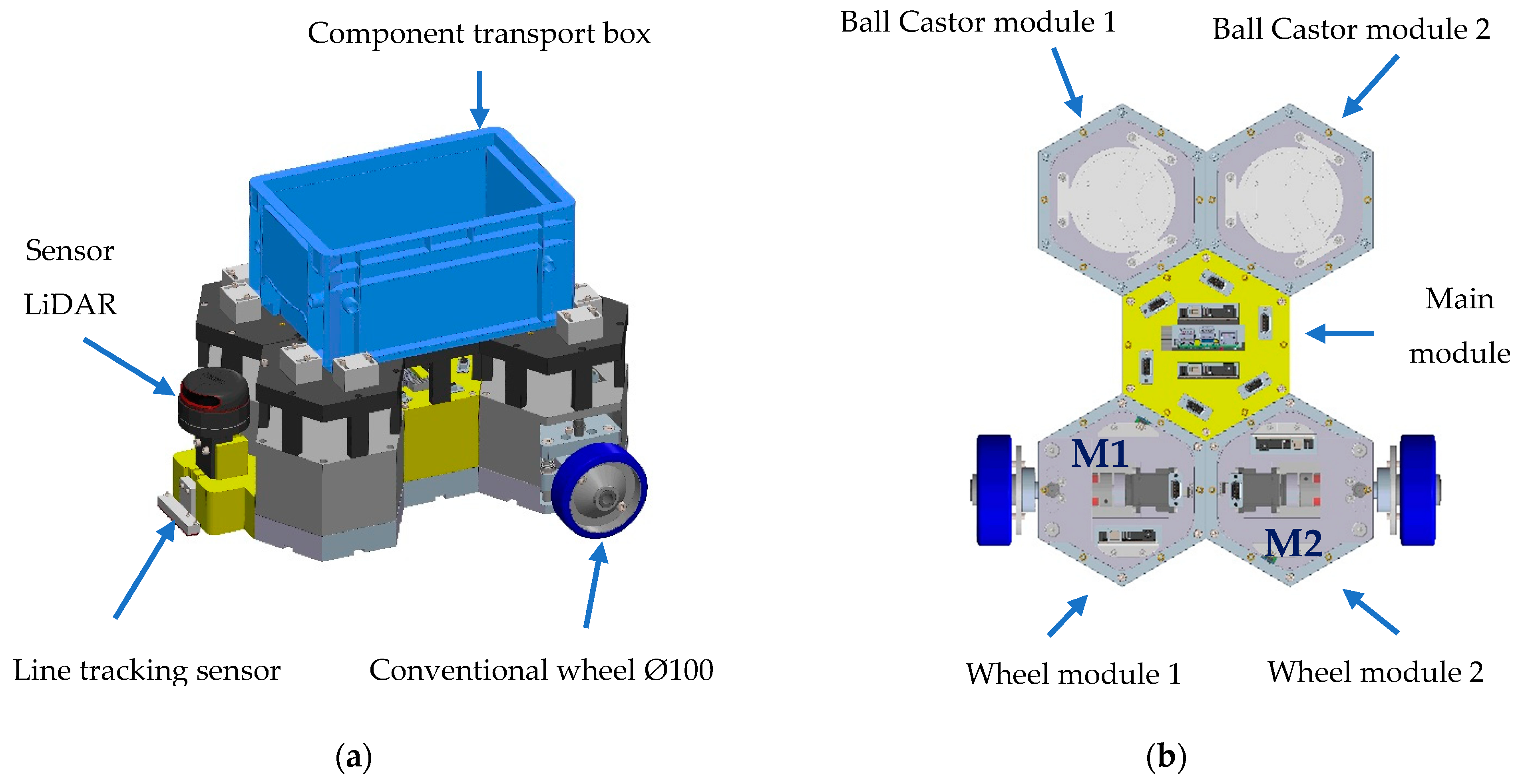
Figure 3.
Modular mobile robot with two conventional wheels (3D model). (a) Isometric view. (b) Top view.
Figure 3.
Modular mobile robot with two conventional wheels (3D model). (a) Isometric view. (b) Top view.
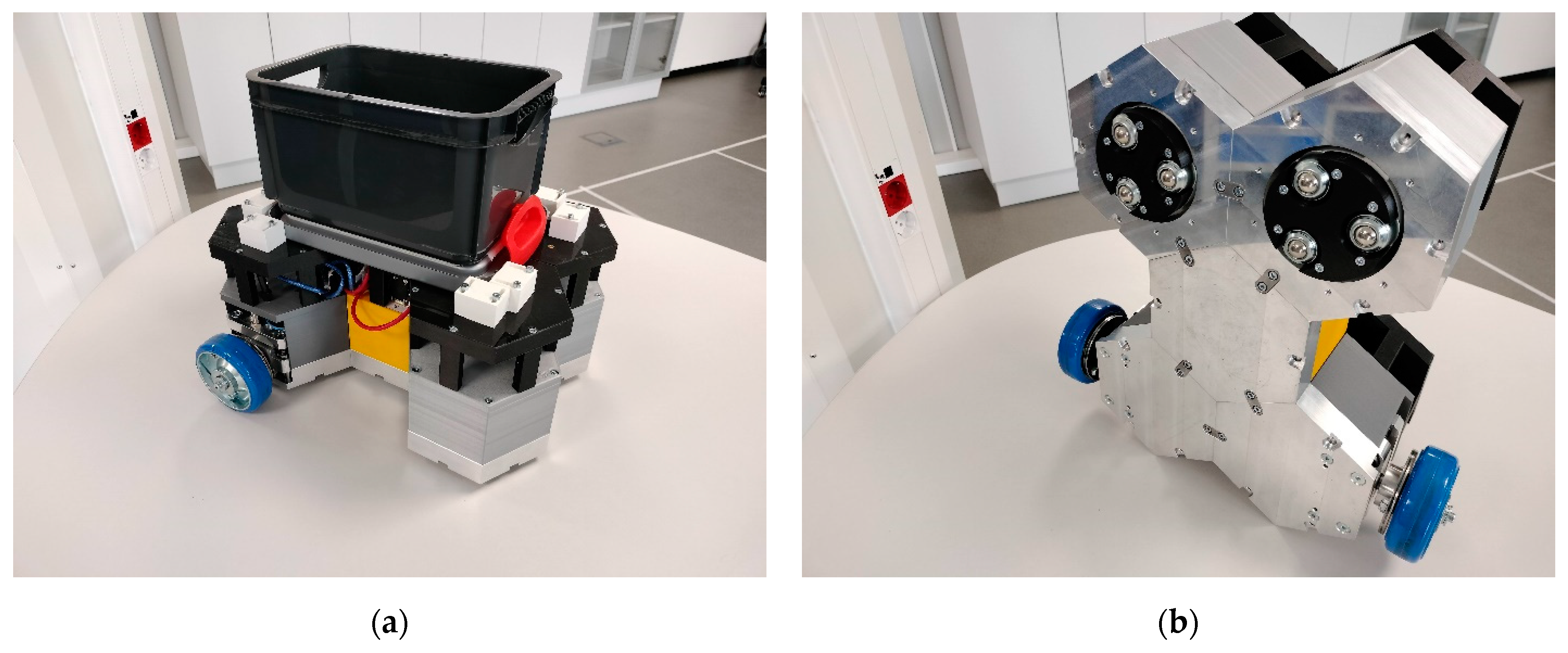
Figure 4.
Modular mobile robot with two conventional wheels (real model). (a) Isometric view. (b) Bottom view.
Figure 4.
Modular mobile robot with two conventional wheels (real model). (a) Isometric view. (b) Bottom view.
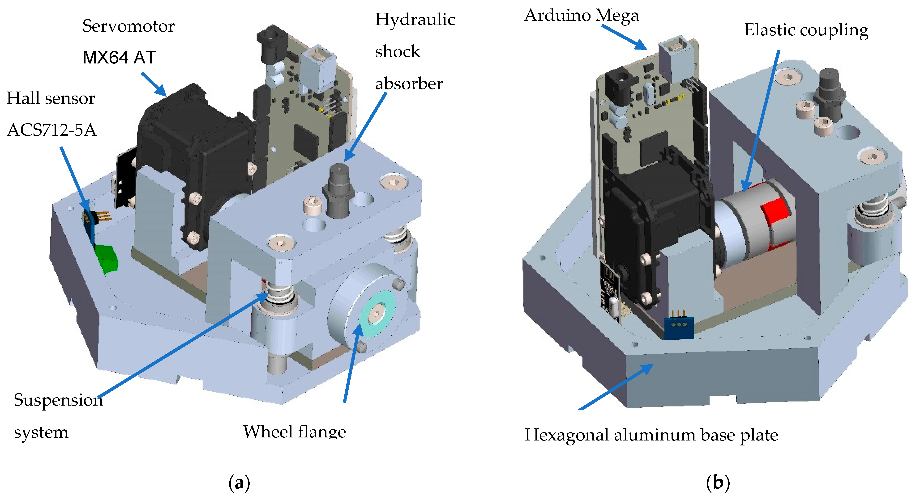
Figure 5.
Drive wheel module of the modular mobile robot (3D model). (a) External view. (b) Internal view.
Figure 5.
Drive wheel module of the modular mobile robot (3D model). (a) External view. (b) Internal view.
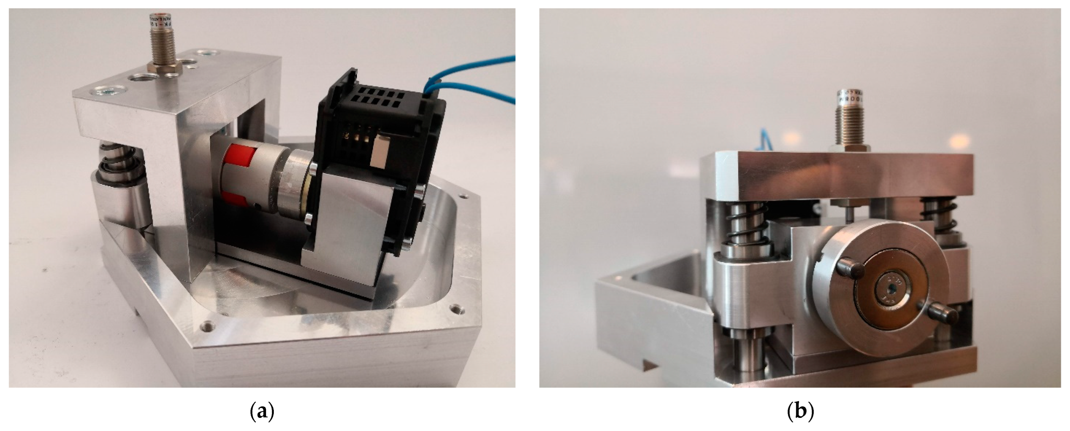
Figure 6.
Drive wheel module assembly (physical model). (a) Internal view. (b) External view.
Figure 6.
Drive wheel module assembly (physical model). (a) Internal view. (b) External view.
Figure 7.
Block diagram of the drive wheel module electric system.
Figure 7.
Block diagram of the drive wheel module electric system.
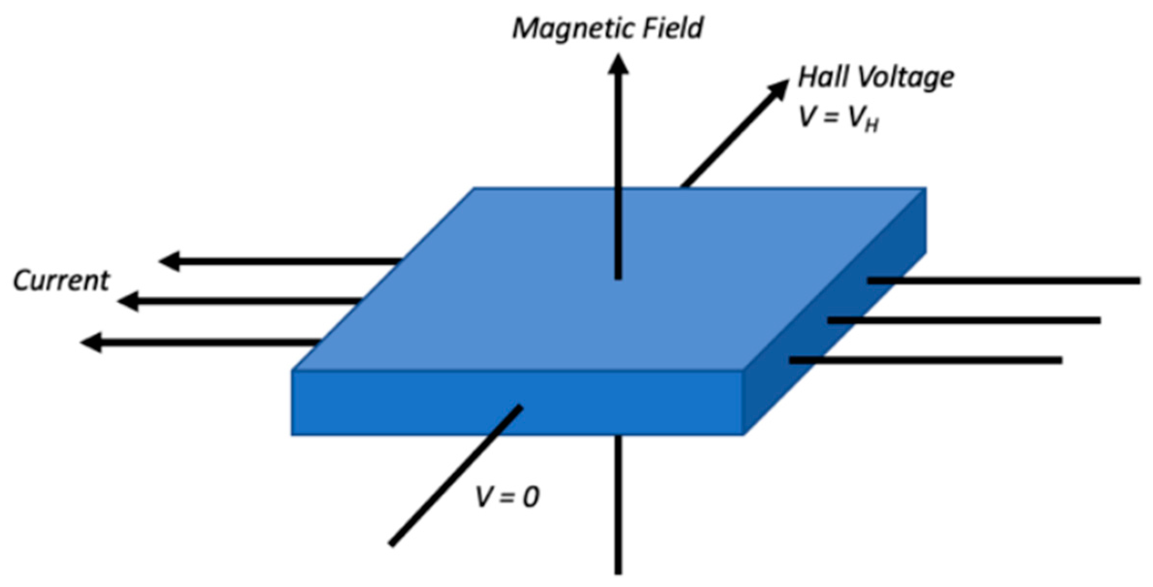
Figure 8.
Hall effect in a thin sheet of conductive material [
43].
Figure 8.
Hall effect in a thin sheet of conductive material [
43].
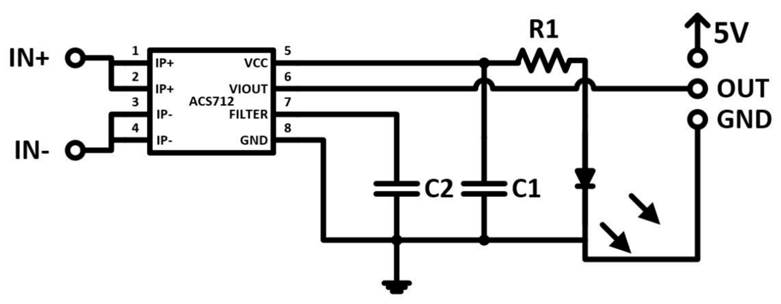
Figure 9.
Electrical diagram of the current sensor [
45].
Figure 9.
Electrical diagram of the current sensor [
45].
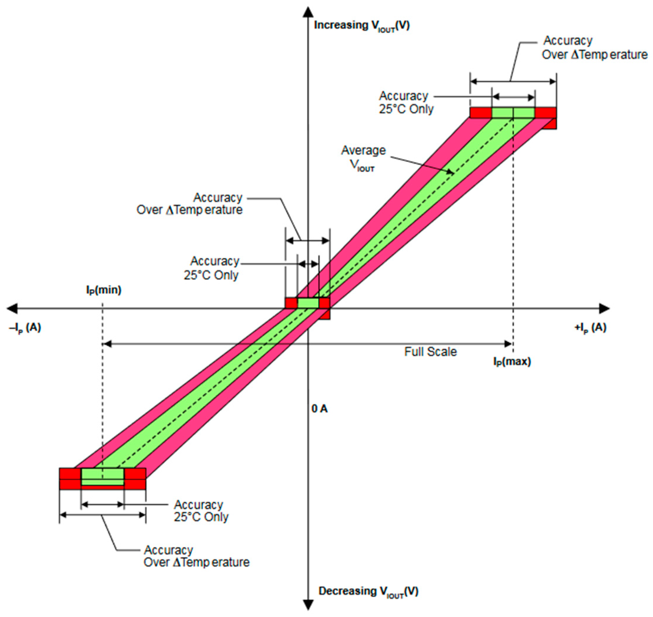
Figure 10.
Current sensor operating curve [
46,
47].
Figure 10.
Current sensor operating curve [
46,
47].
Figure 11.
Electrical diagram of the actuation module.
Figure 11.
Electrical diagram of the actuation module.
Figure 12.
Data acquisition scheme of the drive wheel module and connection with Matalb/Simulink using 10-bit ADC.
Figure 12.
Data acquisition scheme of the drive wheel module and connection with Matalb/Simulink using 10-bit ADC.
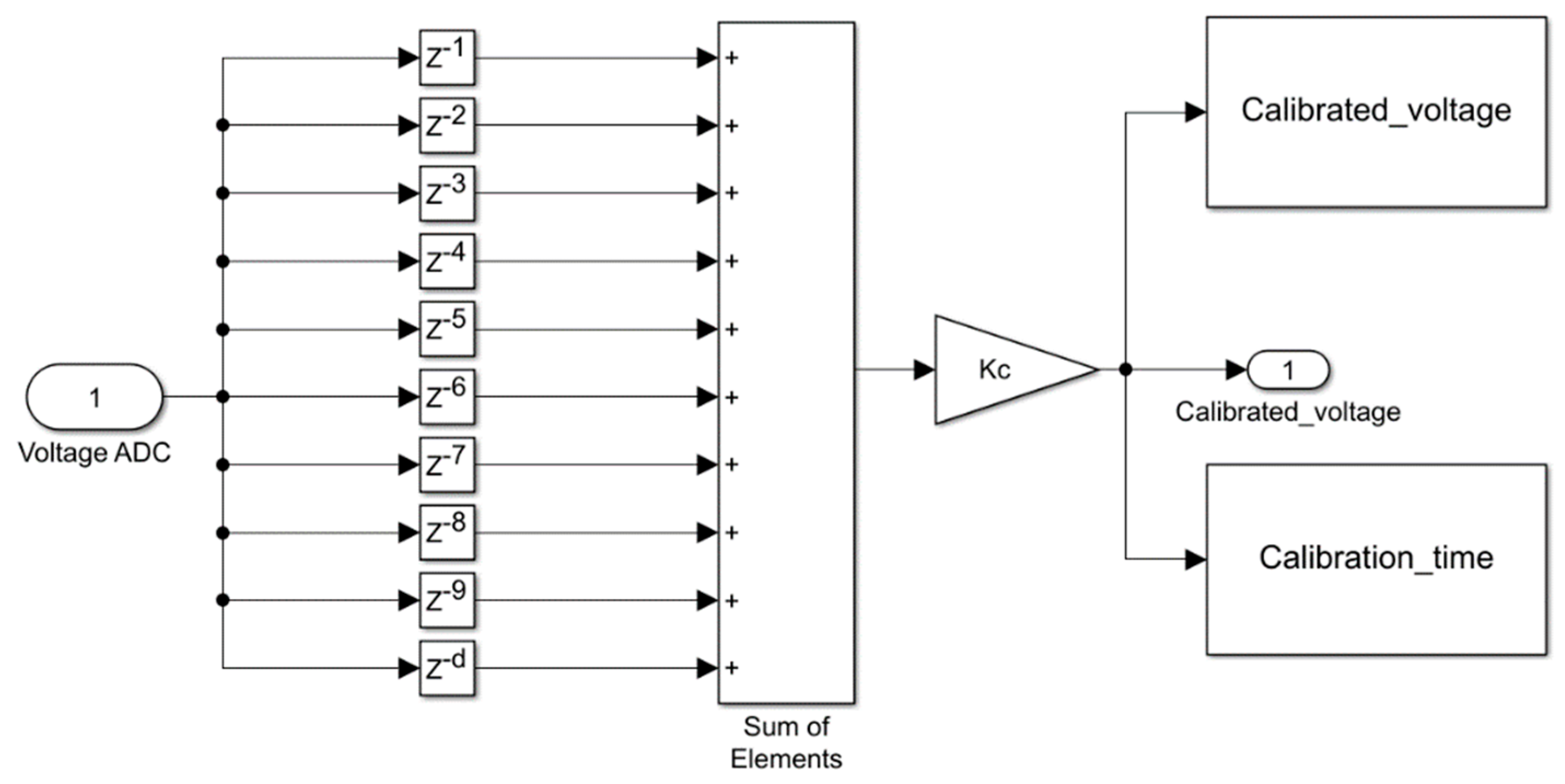
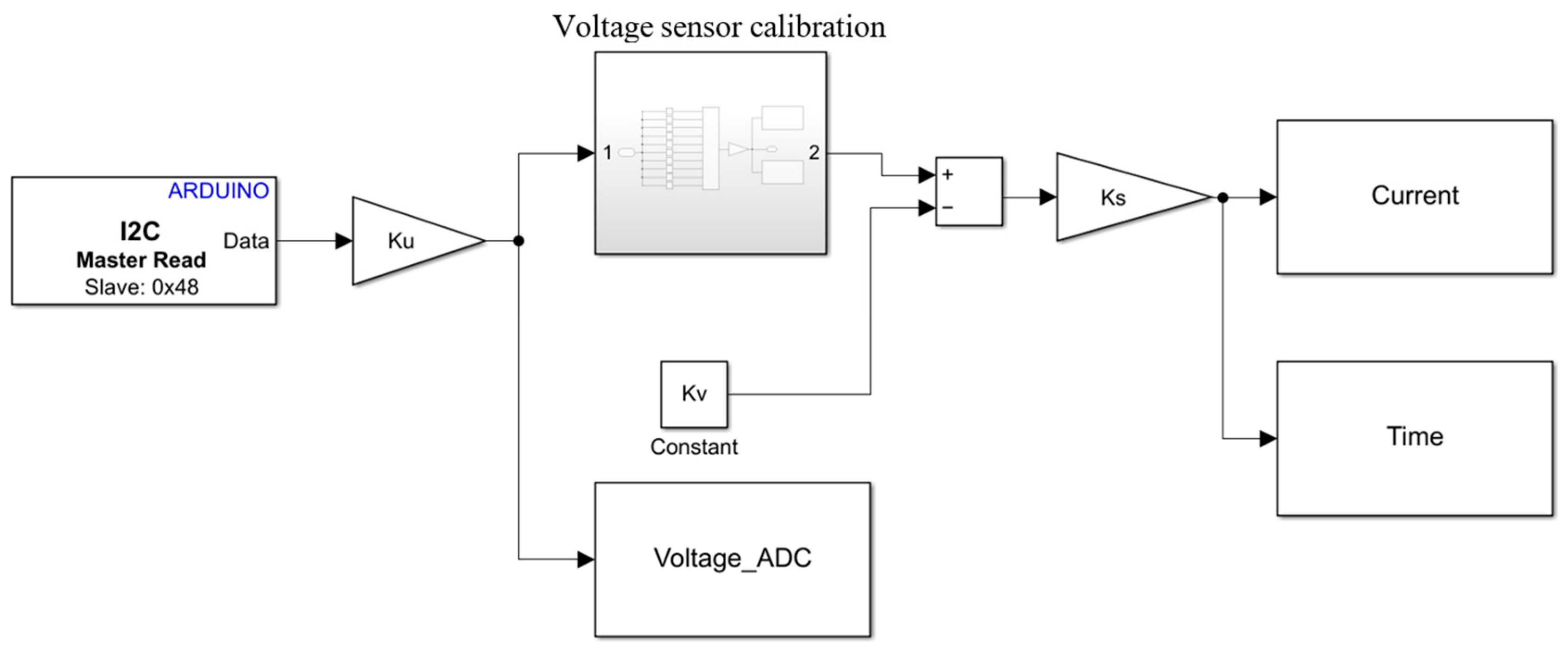
Figure 13.
Voltage sensor calibration.
Figure 13.
Voltage sensor calibration.
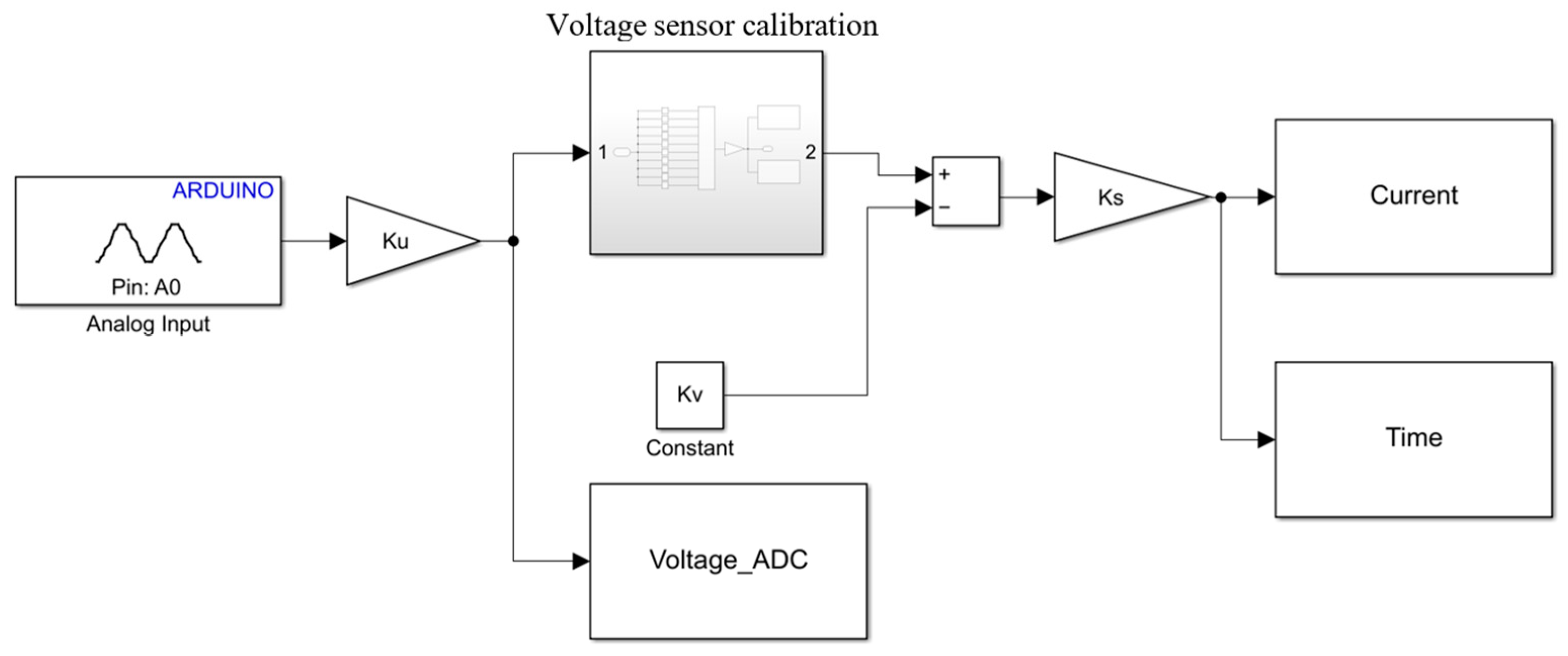
Figure 14.
Simulink model for current monitoring.
Figure 14.
Simulink model for current monitoring.
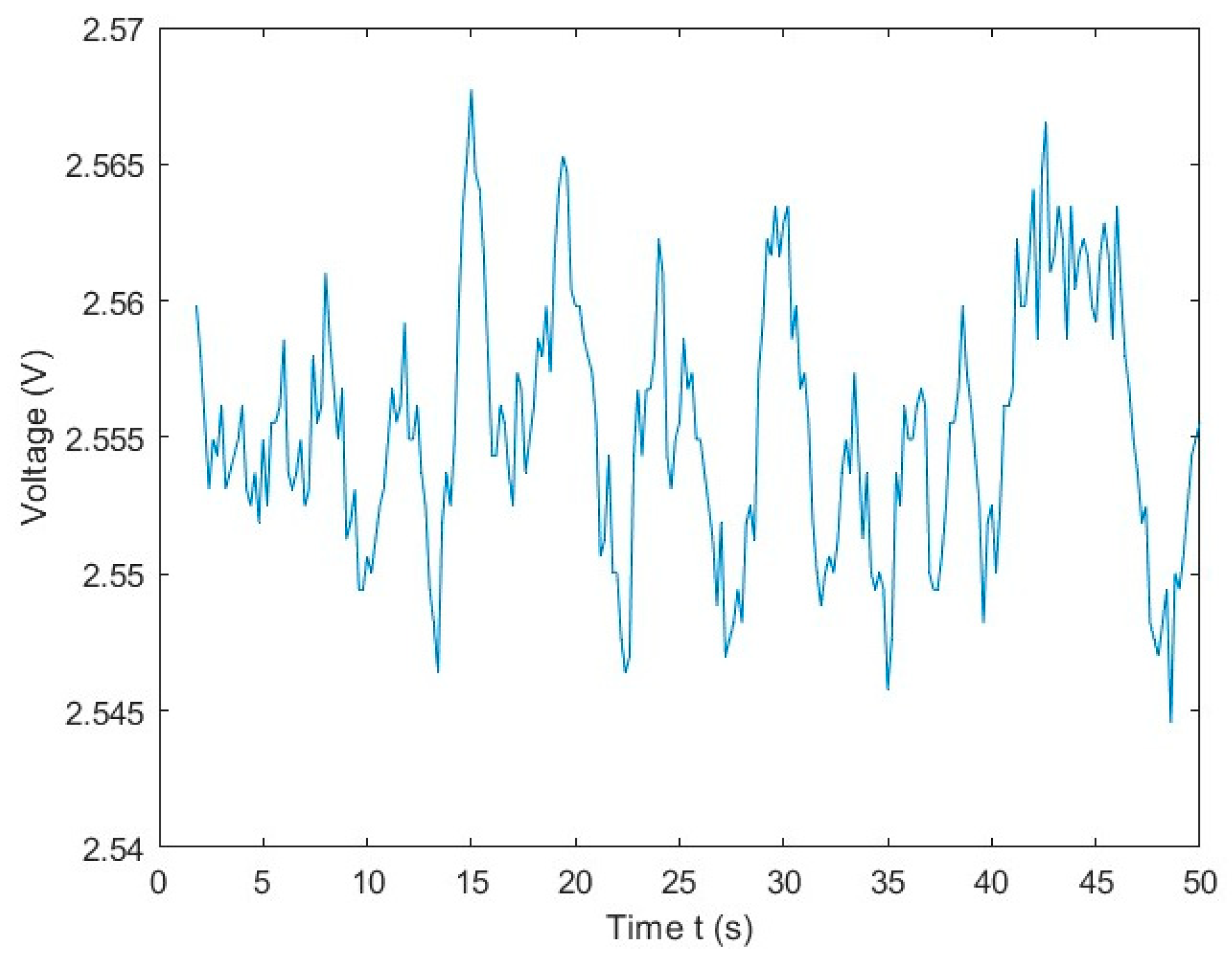
Figure 15.
Voltage variation detected with the ACS712-05 sensor for I = 0 A.
Figure 15.
Voltage variation detected with the ACS712-05 sensor for I = 0 A.
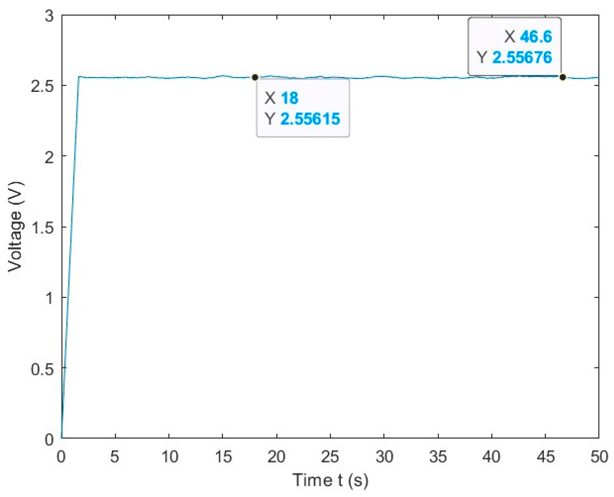
Figure 16.
Voltage variation in the ACS712-05 sensor for I = 0 A after calibration.
Figure 16.
Voltage variation in the ACS712-05 sensor for I = 0 A after calibration.
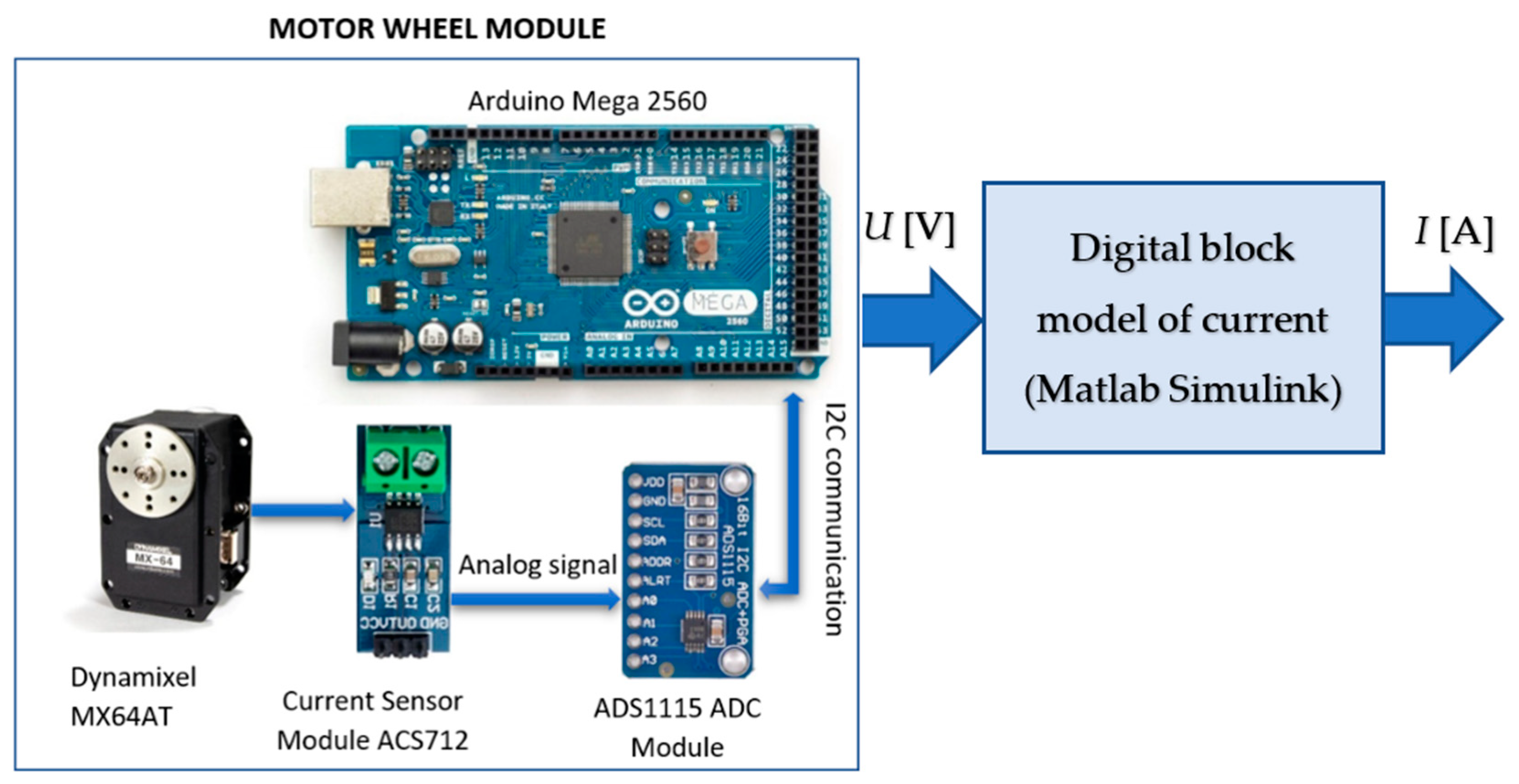
Figure 17.
Motor wheel module data acquisition scheme and Matlab Simulink connection for the 16-bit ADC.
Figure 17.
Motor wheel module data acquisition scheme and Matlab Simulink connection for the 16-bit ADC.
Figure 18.
Simulink model for signal reading using the 16-bit ADC.
Figure 18.
Simulink model for signal reading using the 16-bit ADC.
Figure 19.
ACS712-05 sensor voltage variation for I = 0 A using the 16-bit ADC after calibration.
Figure 19.
ACS712-05 sensor voltage variation for I = 0 A using the 16-bit ADC after calibration.
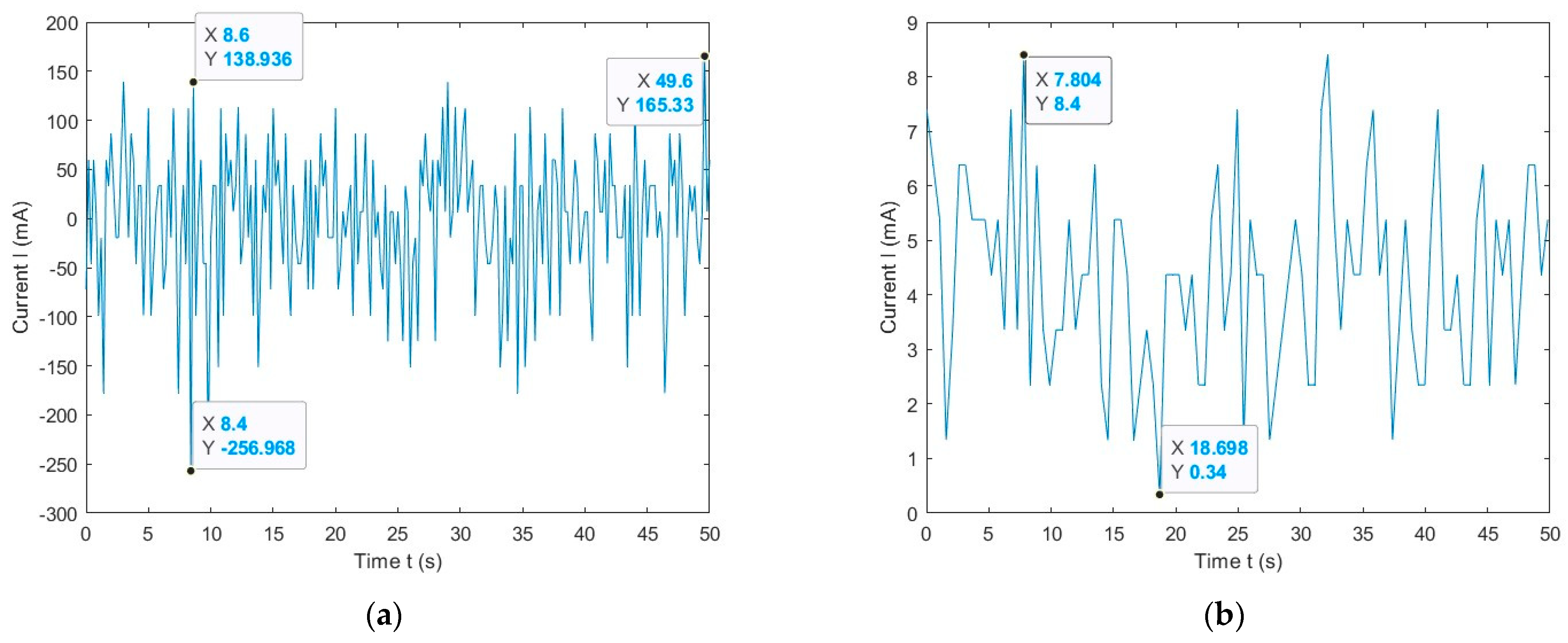
Figure 20.
Variation in the current provided by the ACS712-05 sensor without current consumption: (a) for a 10-bit ADC and (b) for a 16-bit ADC.
Figure 20.
Variation in the current provided by the ACS712-05 sensor without current consumption: (a) for a 10-bit ADC and (b) for a 16-bit ADC.
Figure 21.
Variation in the current provided by the ACS712-05 sensor in the bidirectional operation of the Dynamixel MX64AT servomotor: (a) for a 10-bit ADC and (b) for a 16-bit ADC.
Figure 21.
Variation in the current provided by the ACS712-05 sensor in the bidirectional operation of the Dynamixel MX64AT servomotor: (a) for a 10-bit ADC and (b) for a 16-bit ADC.
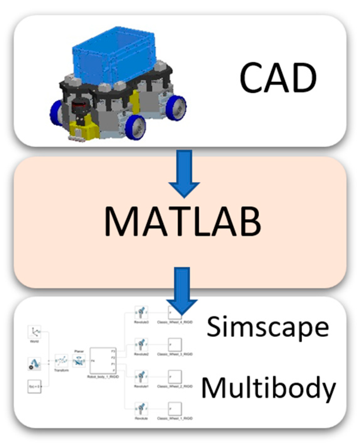
Figure 22.
The connection between the 3D CAD model and Simulink–Simscape–Multibody.
Figure 22.
The connection between the 3D CAD model and Simulink–Simscape–Multibody.
Figure 23.
Result of the CAD model import in Simulink Simscape.
Figure 23.
Result of the CAD model import in Simulink Simscape.
Figure 24.
The 3D model of the mobile robot in Simulink Simscape. (a) Top view. (b) Isometric view. (c) Lateral view.
Figure 24.
The 3D model of the mobile robot in Simulink Simscape. (a) Top view. (b) Isometric view. (c) Lateral view.
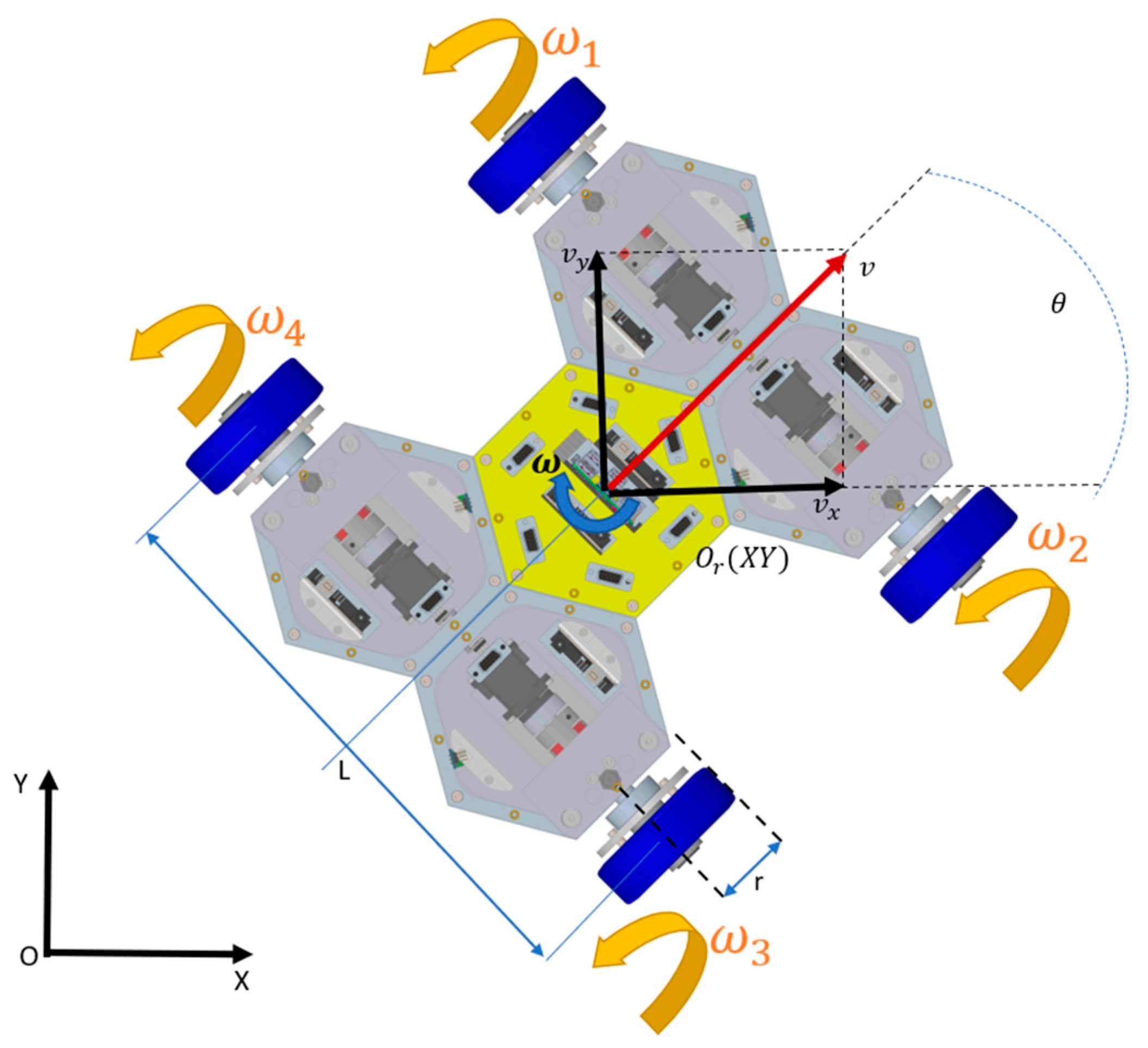
Figure 25.
Schematic kinematic model of the modular mobile robot with differential traction.
Figure 25.
Schematic kinematic model of the modular mobile robot with differential traction.
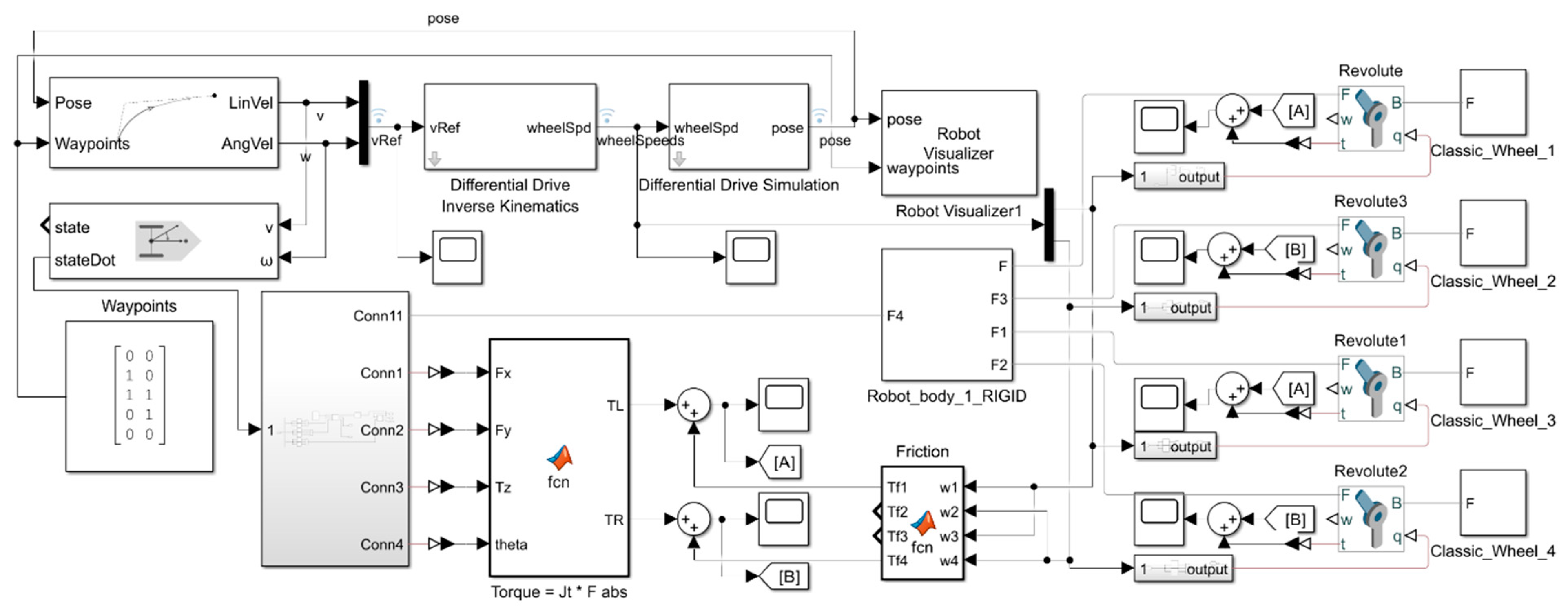
Figure 26.
Dynamic model of the mobile robot—block diagram.
Figure 26.
Dynamic model of the mobile robot—block diagram.
Figure 27.
The path traveled by the robot. (a) Trajectory resulting from the simulation. (b) The 90° turn of the robot in the simulation.
Figure 27.
The path traveled by the robot. (a) Trajectory resulting from the simulation. (b) The 90° turn of the robot in the simulation.
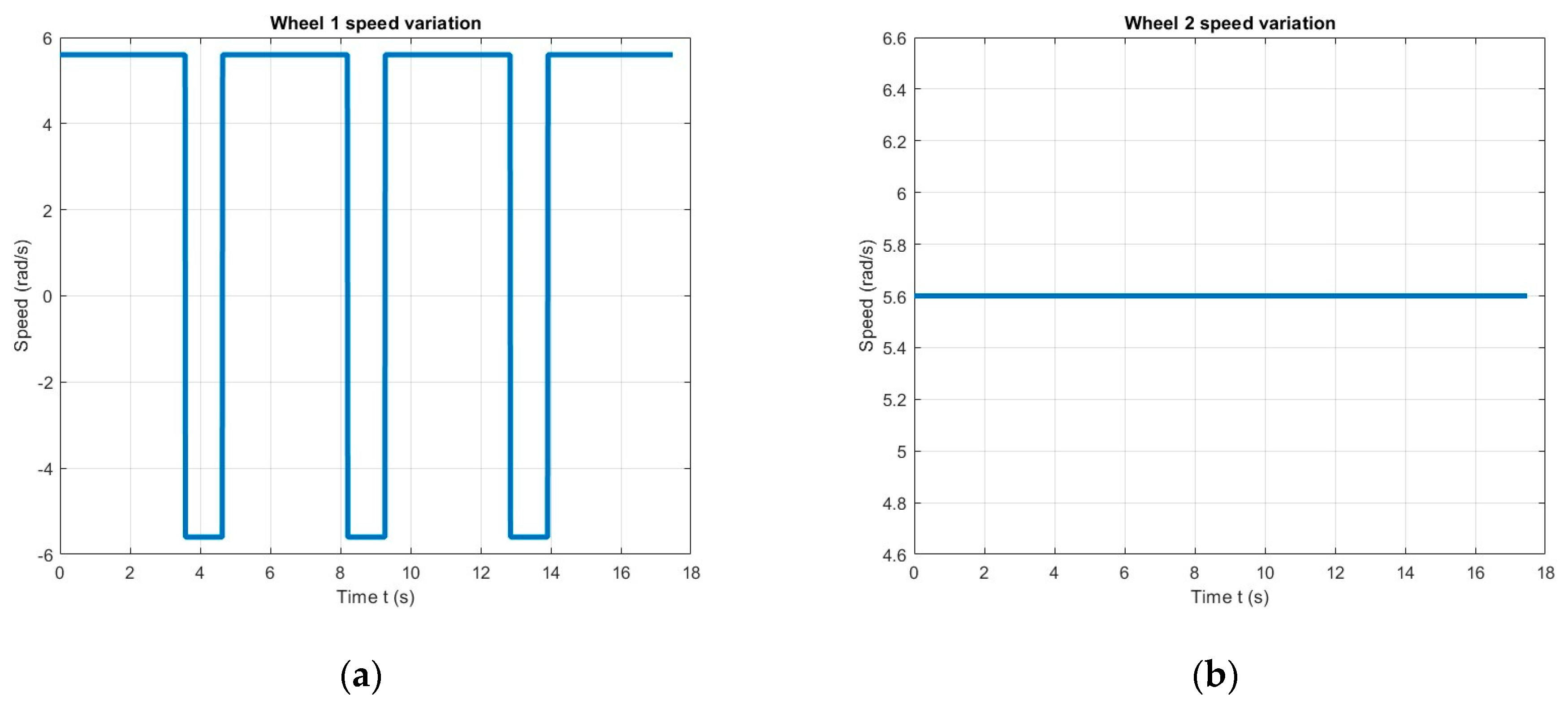
Figure 28.
Variations in the input speeds in the dynamic model of the wheels. (a) For wheel 1 (similar to wheel 3). (b) For wheel 2 (similar to wheel 4).
Figure 28.
Variations in the input speeds in the dynamic model of the wheels. (a) For wheel 1 (similar to wheel 3). (b) For wheel 2 (similar to wheel 4).
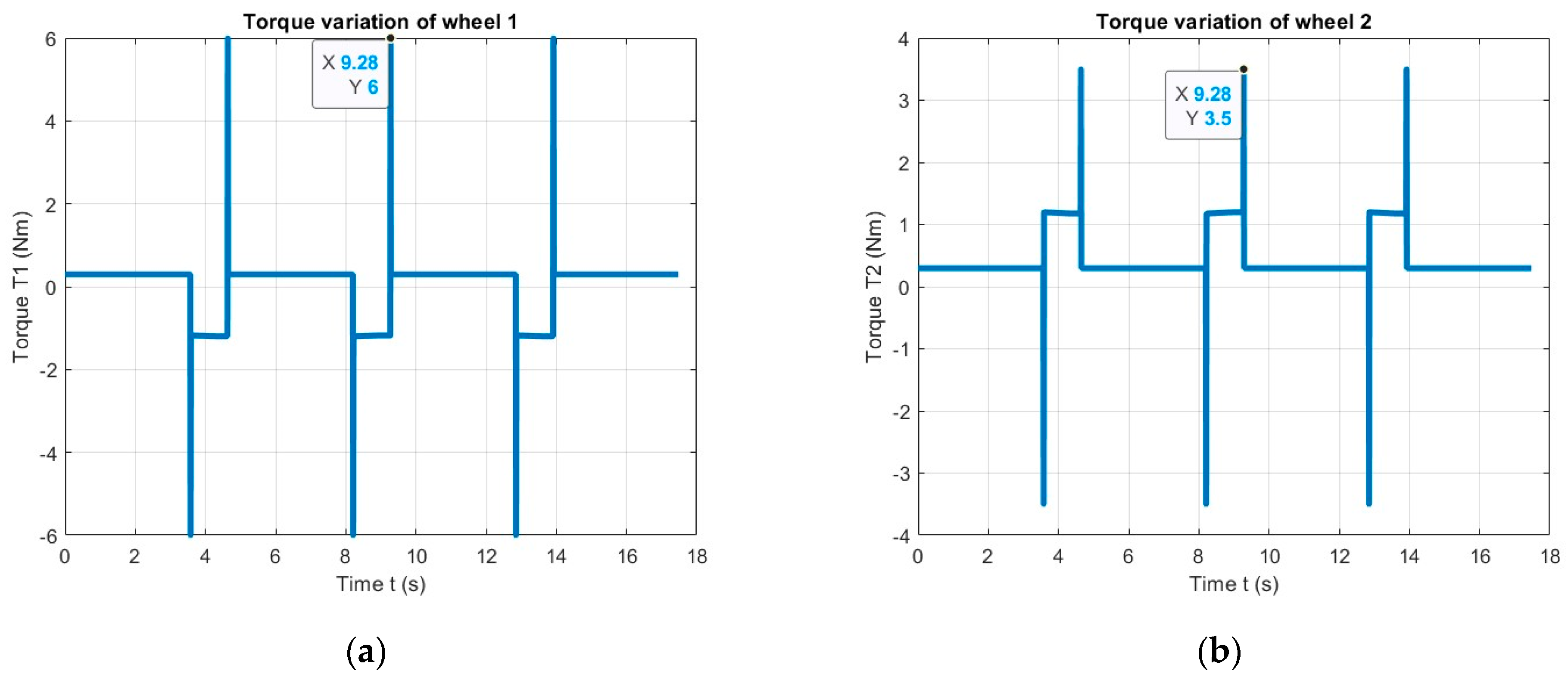
Figure 29.
Torque variation for a 1 m square trajectory. (a) Wheel 1 (similar to wheel 3). (b) Wheel 2 (similar to wheel 4).
Figure 29.
Torque variation for a 1 m square trajectory. (a) Wheel 1 (similar to wheel 3). (b) Wheel 2 (similar to wheel 4).
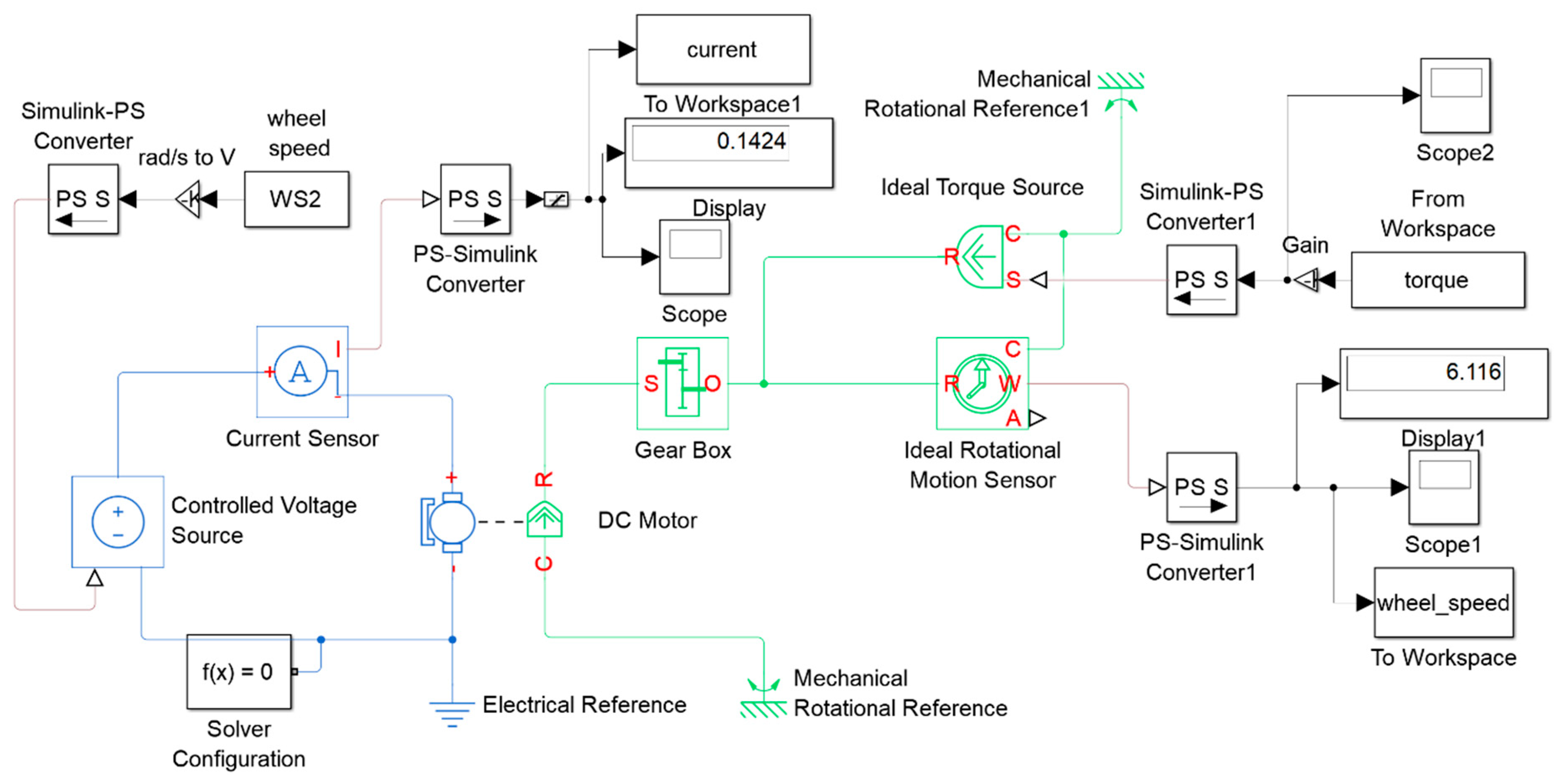
Figure 30.
Block diagram of the actuation system.
Figure 30.
Block diagram of the actuation system.
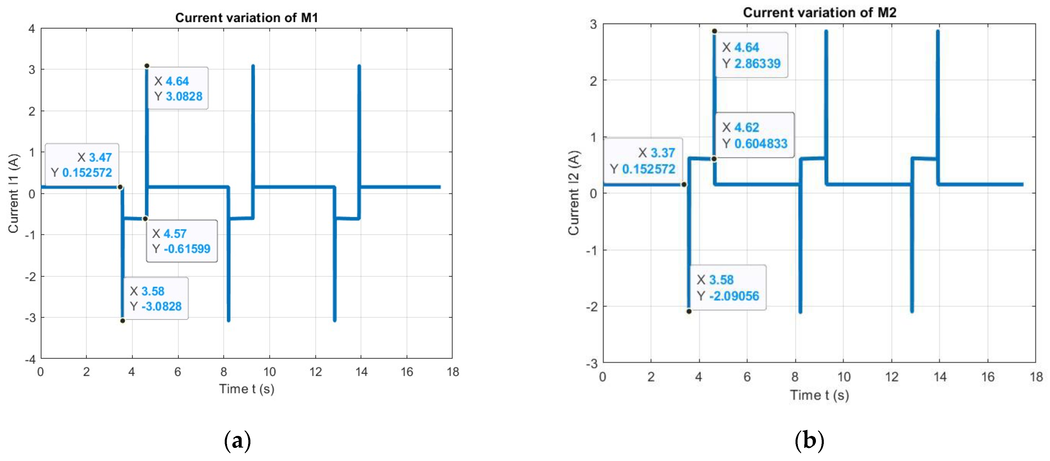
Figure 31.
Current variation determined in the model simulation for a 1 m square trajectory. (a) Wheel 1 (similar to wheel 3). (b) Wheel 2 (similar to wheel 4).
Figure 31.
Current variation determined in the model simulation for a 1 m square trajectory. (a) Wheel 1 (similar to wheel 3). (b) Wheel 2 (similar to wheel 4).
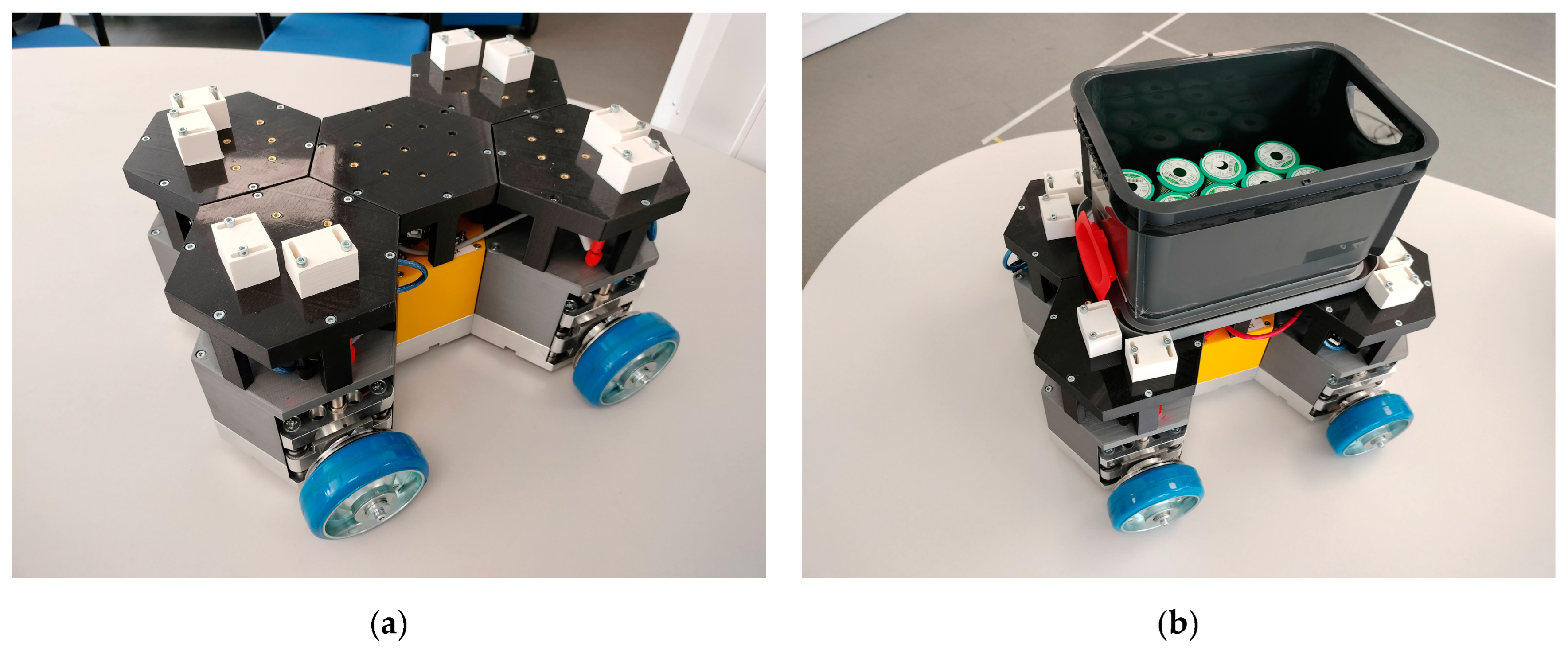
Figure 32.
Modular mobile robot with conventional four wheels. (a) Without transport box. (b) With load carried.
Figure 32.
Modular mobile robot with conventional four wheels. (a) Without transport box. (b) With load carried.
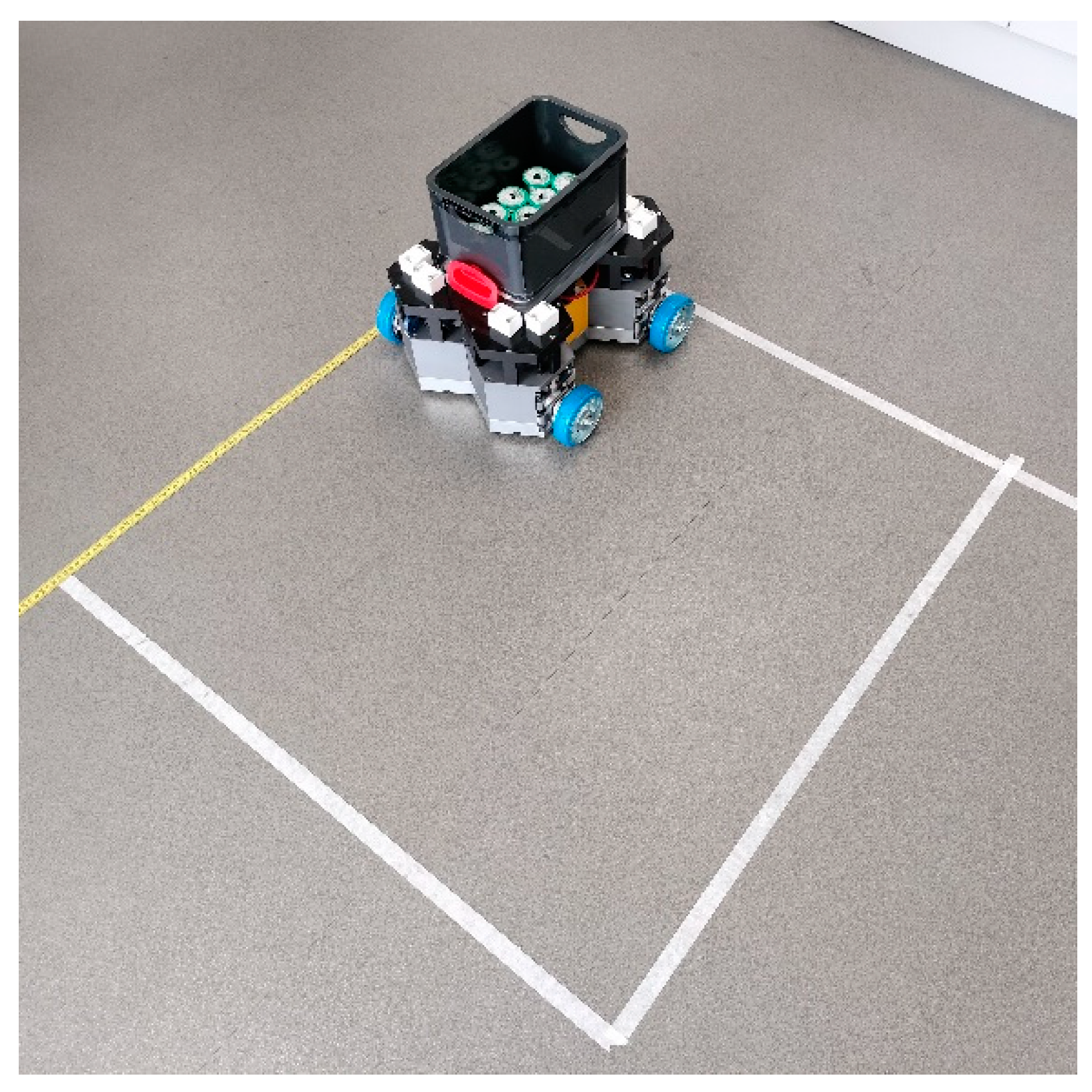
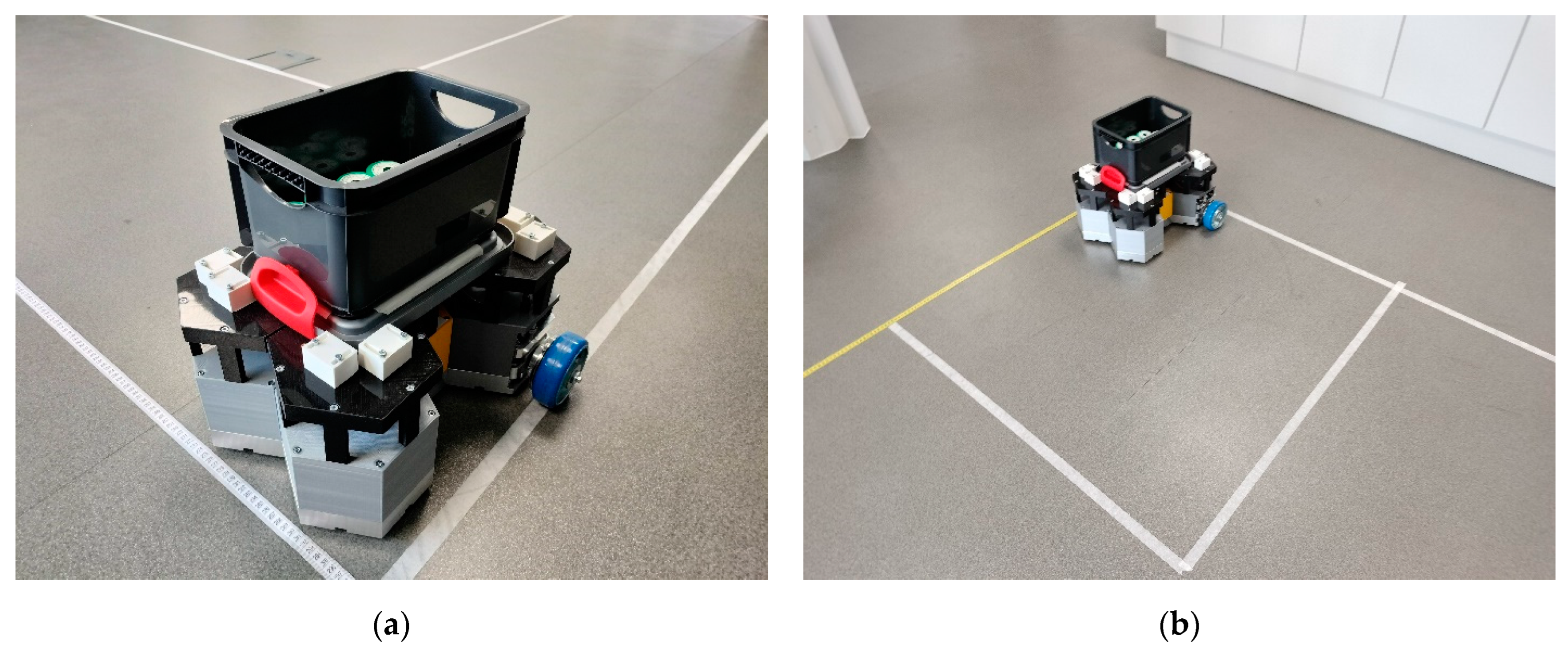
Figure 33.
Physical path and real mobile robot.
Figure 33.
Physical path and real mobile robot.
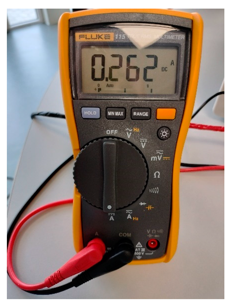
Figure 34.
Fluke 115 Digital Multimeter.
Figure 34.
Fluke 115 Digital Multimeter.
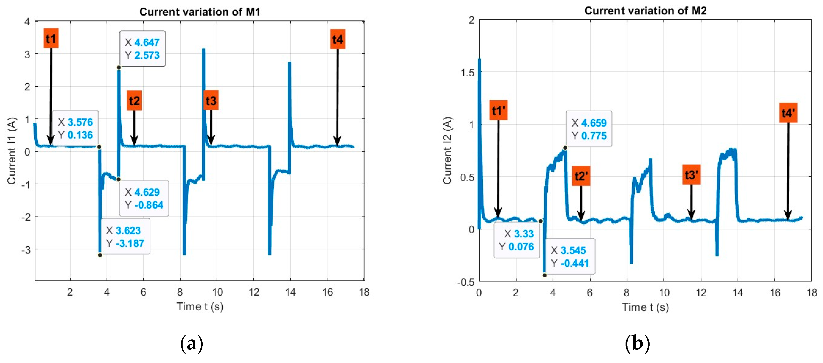
Figure 35.
Current variation measured using the functional model for moving on the redefined path. (a) Wheel 1 (similar to wheel 3). (b) Wheel 2 (similar to wheel 4).
Figure 35.
Current variation measured using the functional model for moving on the redefined path. (a) Wheel 1 (similar to wheel 3). (b) Wheel 2 (similar to wheel 4).
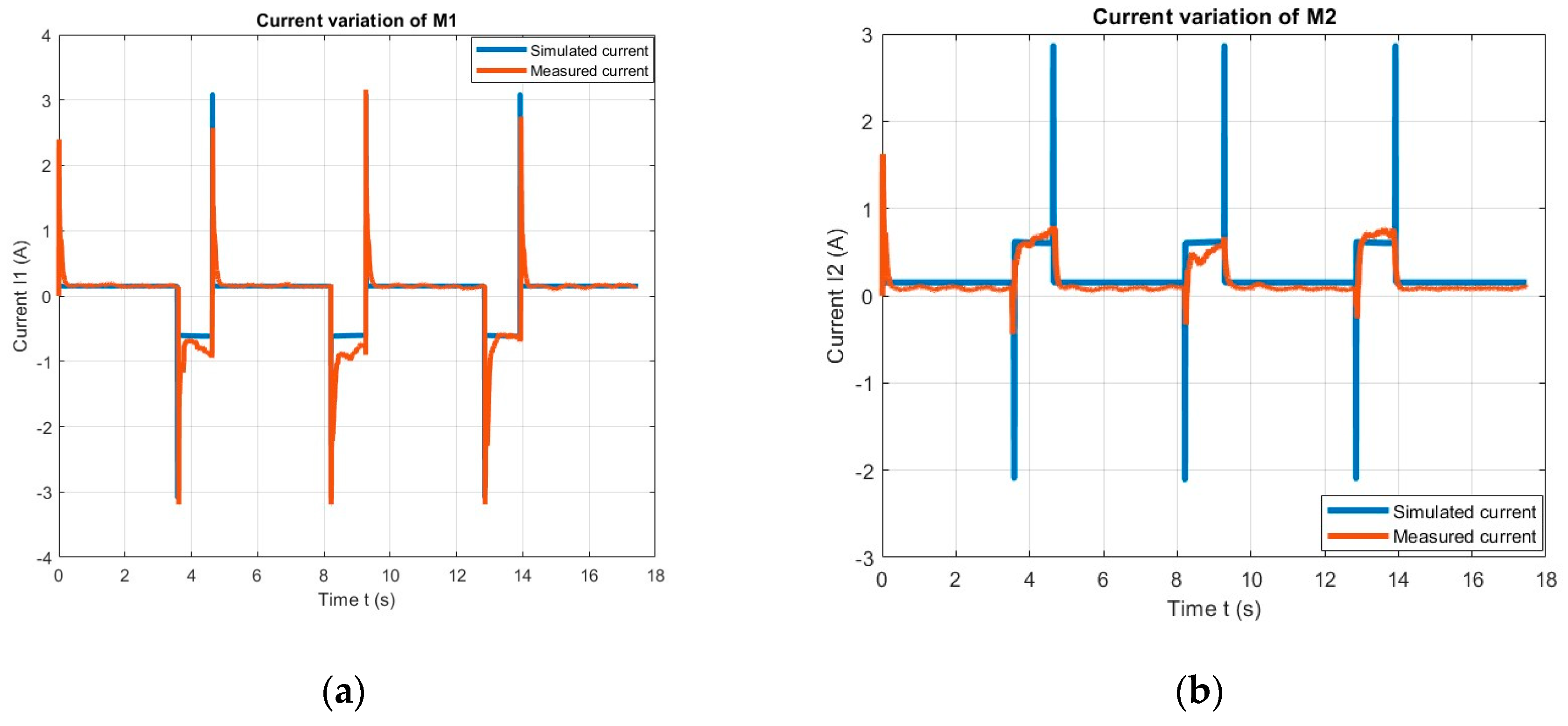
Figure 36.
Variation in the simulated and measured current. (a) Wheel 1 (similar to wheel 3). (b) Wheel 2 (similar to wheel 4).
Figure 36.
Variation in the simulated and measured current. (a) Wheel 1 (similar to wheel 3). (b) Wheel 2 (similar to wheel 4).
Figure 37.
Physical path and real mobile robot. (a) Close view. (b) Mobile robot on the path.
Figure 37.
Physical path and real mobile robot. (a) Close view. (b) Mobile robot on the path.
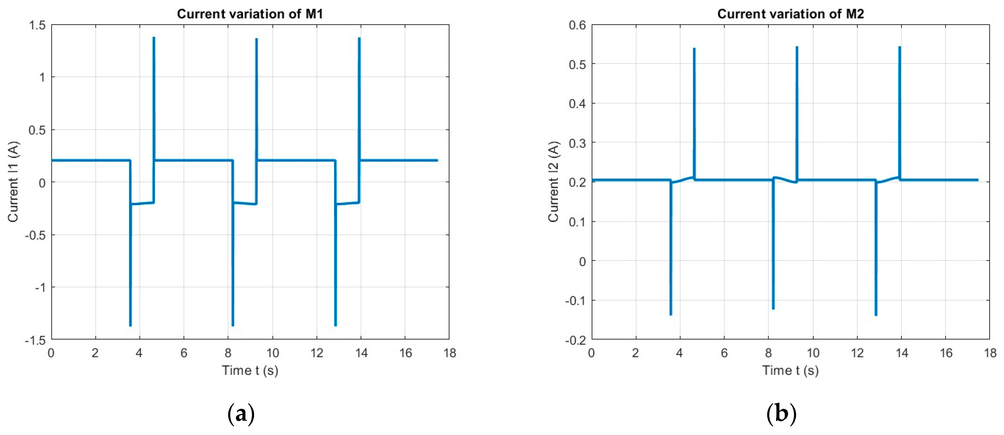
Figure 38.
Current variation simulated for a 1 m square path. (a) Wheel 1. (b) Wheel 2.
Figure 38.
Current variation simulated for a 1 m square path. (a) Wheel 1. (b) Wheel 2.
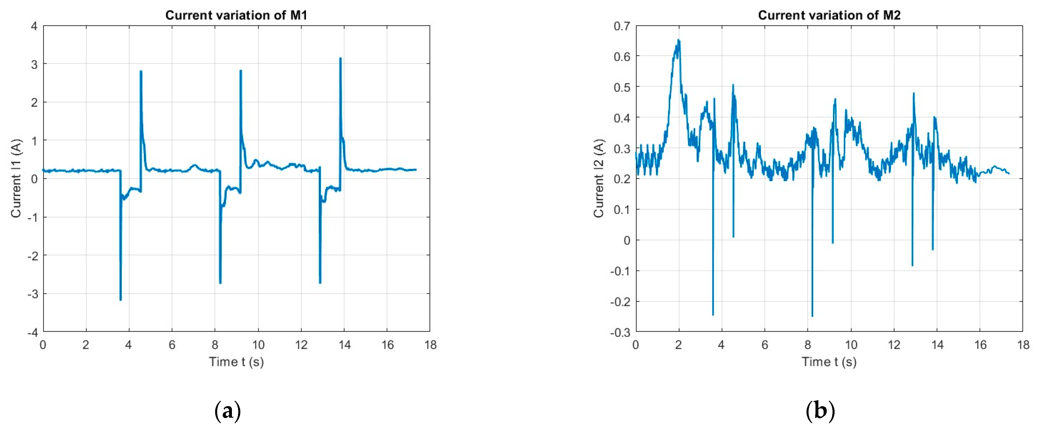
Figure 39.
Current variation measured using the functional model for moving on the predefined path. (a) Wheel 1. (b) Wheel 2.
Figure 39.
Current variation measured using the functional model for moving on the predefined path. (a) Wheel 1. (b) Wheel 2.
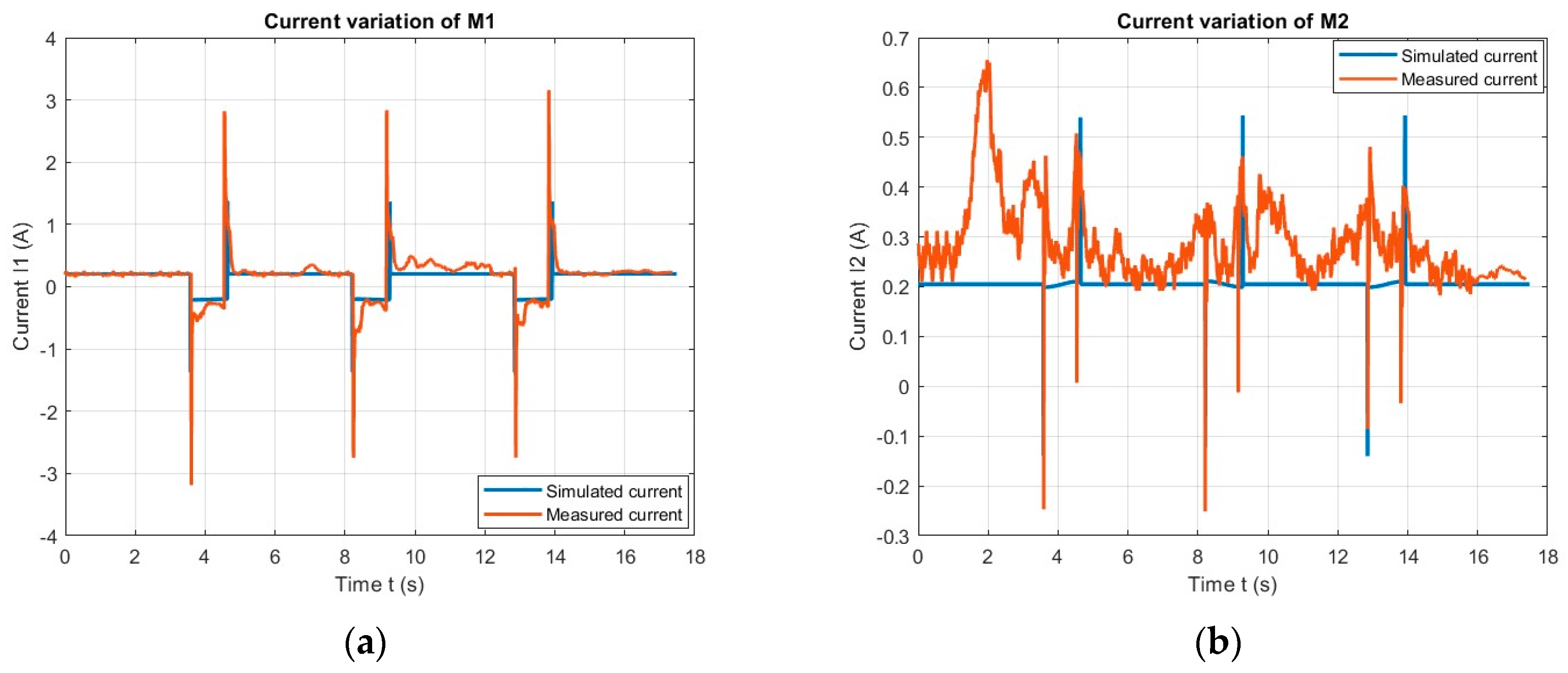
Figure 40.
Variation in the simulated and measured current. (a) Wheel 1. (b) Wheel 2.
Figure 40.
Variation in the simulated and measured current. (a) Wheel 1. (b) Wheel 2.
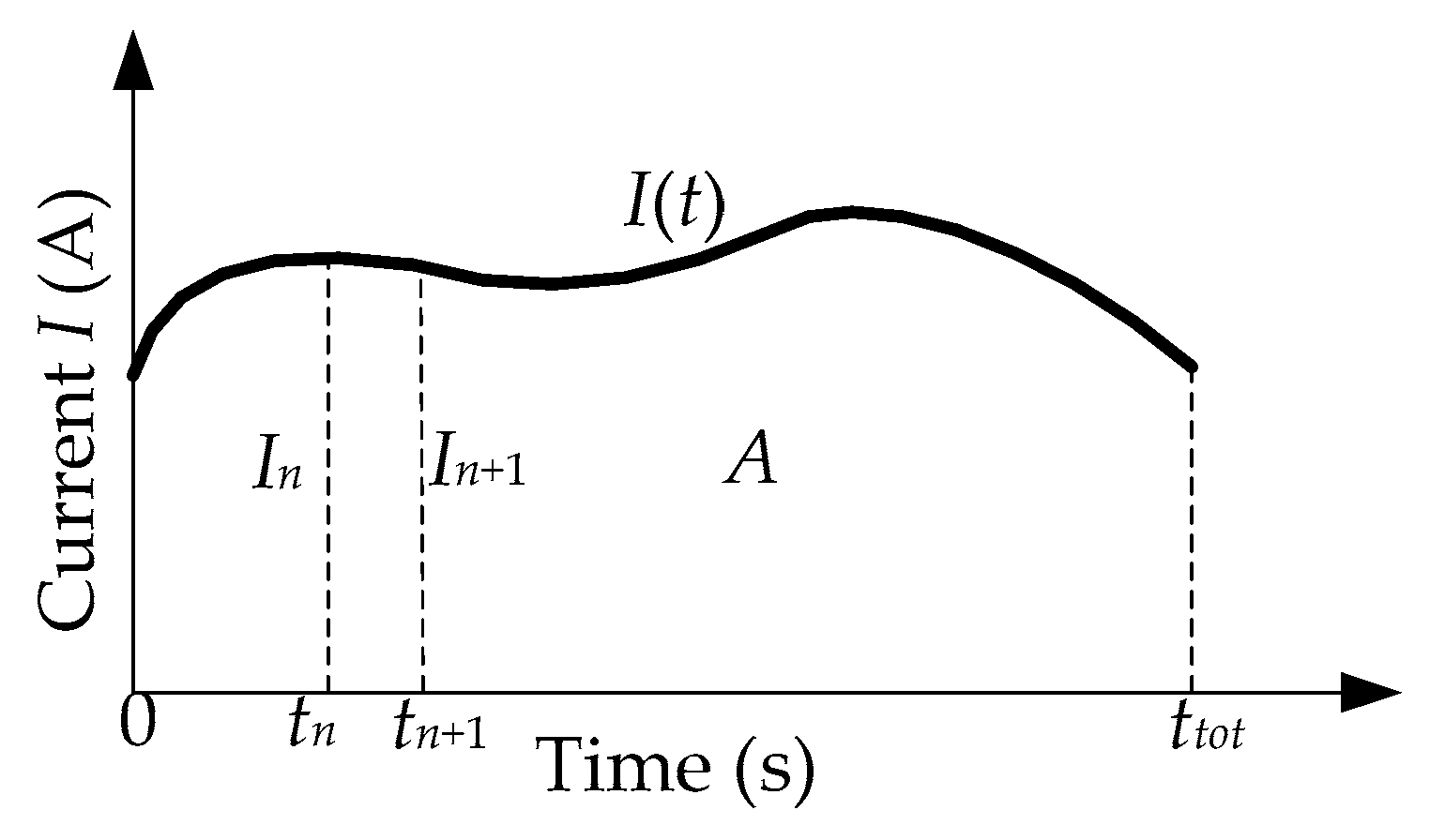
Figure 41.
Calculation of the definite integral.
Figure 41.
Calculation of the definite integral.
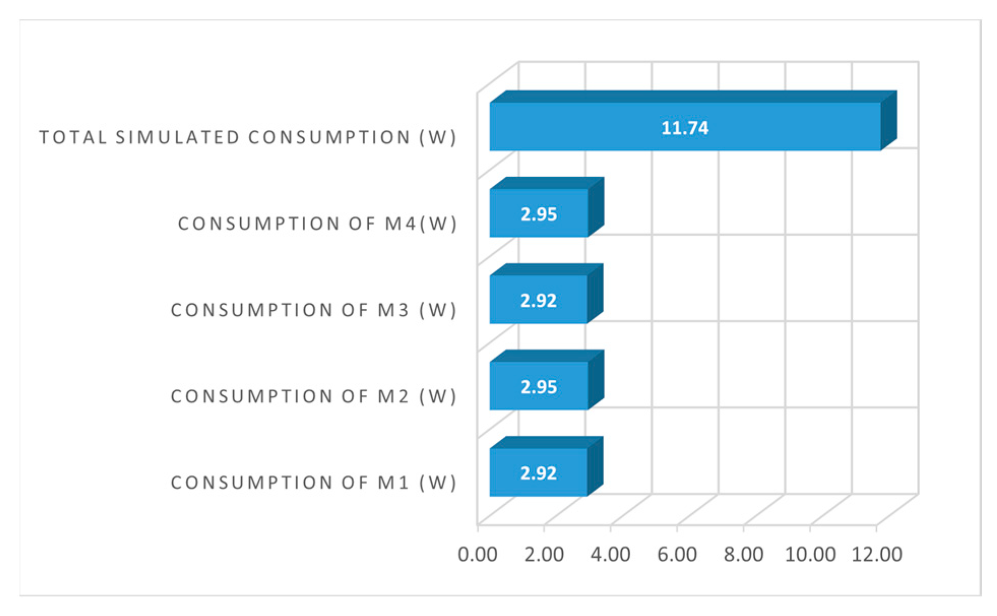
Figure 42.
Power consumption—simulated in the case of the four-wheeled robot.
Figure 42.
Power consumption—simulated in the case of the four-wheeled robot.
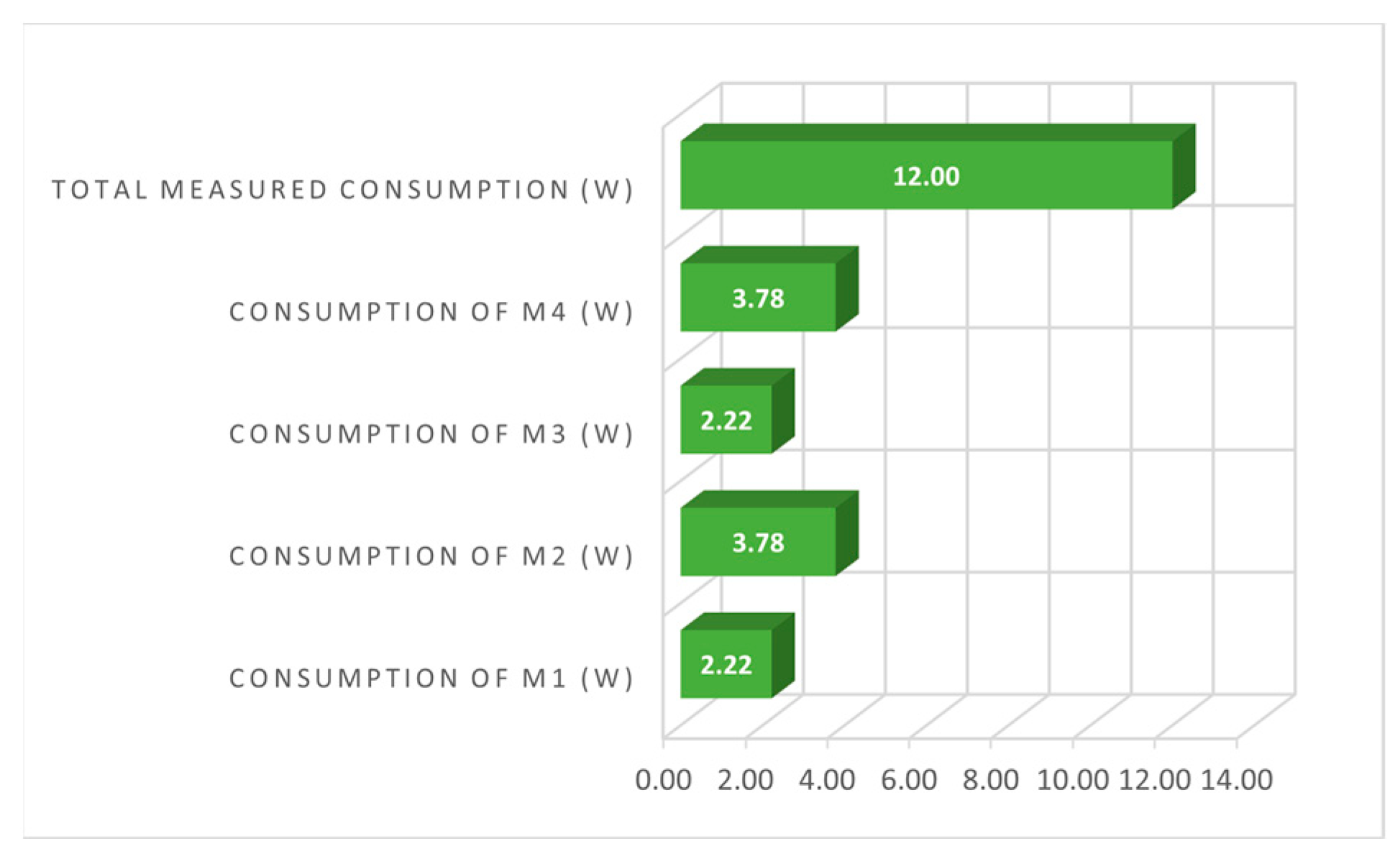
Figure 43.
Power consumption—measured in the case of the four-wheeled robot.
Figure 43.
Power consumption—measured in the case of the four-wheeled robot.
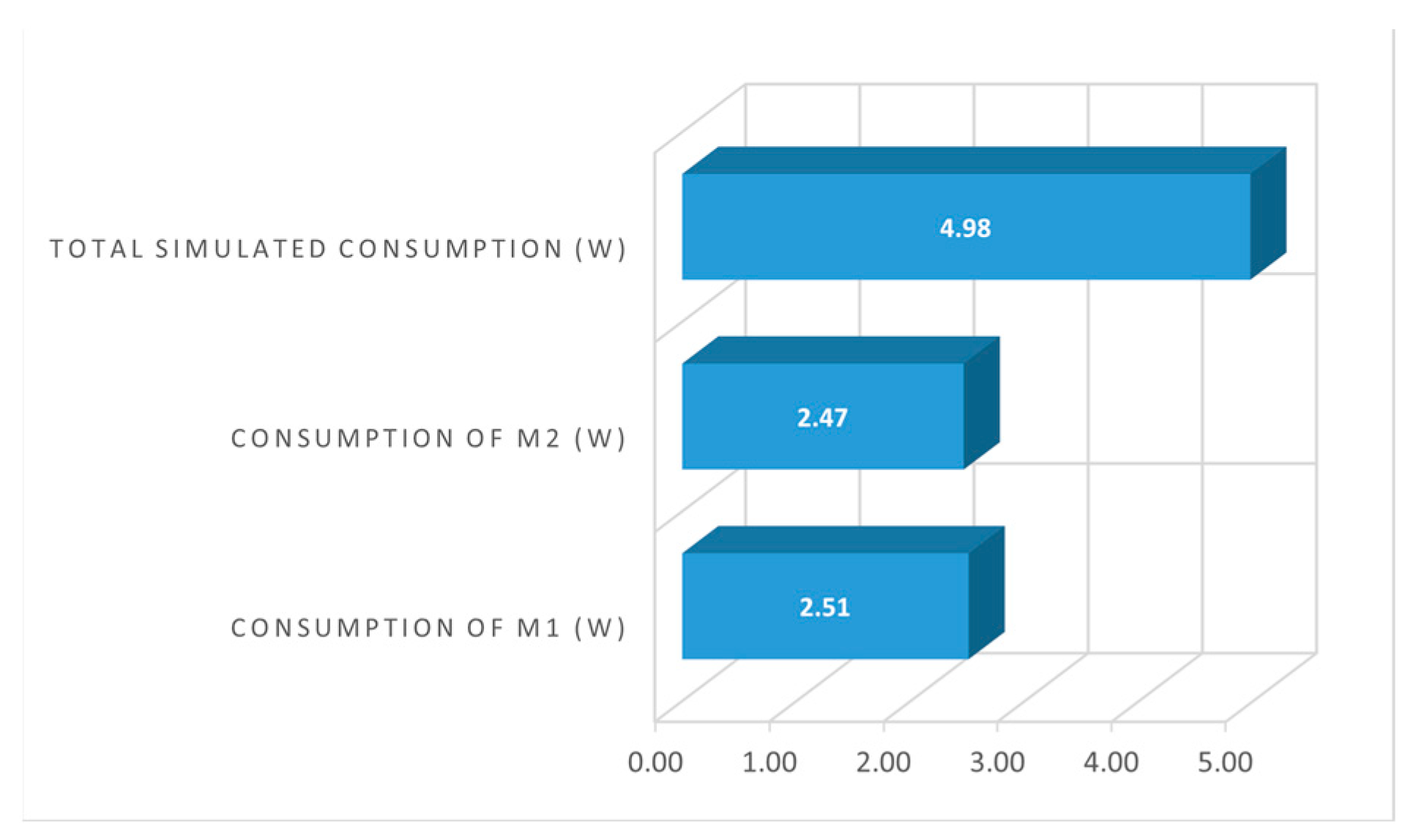
Figure 44.
Power consumption—simulated in the case of the two-wheeled robot.
Figure 44.
Power consumption—simulated in the case of the two-wheeled robot.
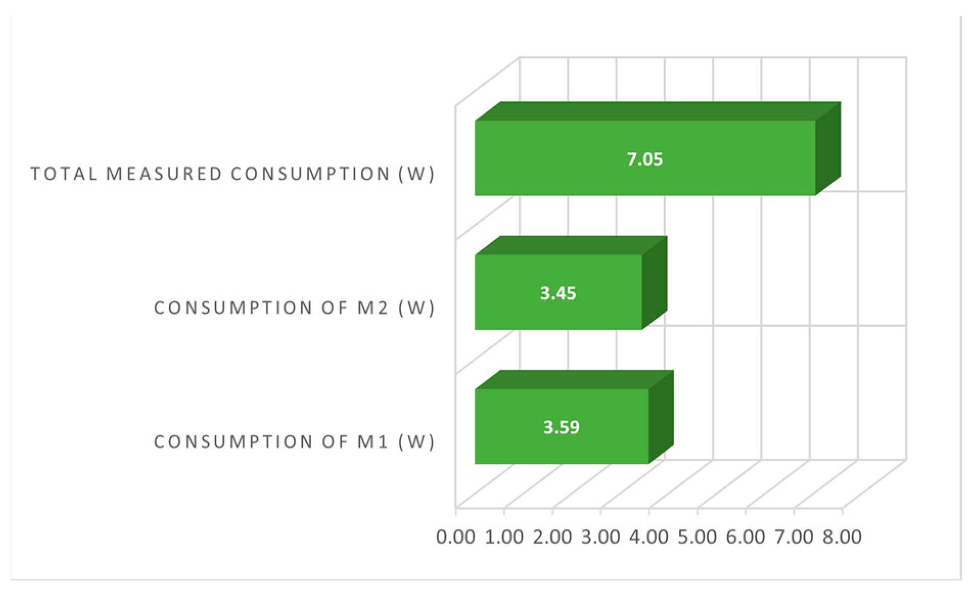
Figure 45.
Power consumption—measured in the case of the two-wheeled robot.
Figure 45.
Power consumption—measured in the case of the two-wheeled robot.
Table 1.
References of the state of the art on sections.
Table 1.
References of the state of the art on sections.
| Title [Source] | Document Type | Cited Reference Count | Times Cited, All Databases | Year | Categories |
|---|
| General aspects of mobile robots |
| Mobile Robots Locomotion [17] | Review | 73 | 3 | 2022 | Engineering, Mechanical |
| Wheeled mobile robot [18] | Review | 118 | 2 | 2021 | Disciplines, Multidisciplinary |
| Omnidirectional mobile robots [19] | Article | 354 | 21 | 2020 | Engineering, Mechanical |
| Navigation of mobile robot [20] | Review | 208 | 220 | 2019 | Engineering, Multidisciplinary |
| A review of mobile robots [8] | Review | 188 | 120 | 2019 | Robotics |
| Hall sensors |
| Hall-Effect Current Sensors [21] | Article | 103 | 6 | 2022 | Engineering, Applied |
| Photo-Induced Hall Sensors [22] | Article | 34 | 3 | 2021 | Engineering, Electrical |
| Current Sensors [23] | Article | 21 | 15 | 2019 | Engineering, Electrical |
| Wireless Current Monitoring [24] | C. Paper | 8 | 0 | 2019 | Engineering, Electrical |
| MagFET-current sensor [25] | Article | 23 | 14 | 2013 | Engineering, Electrical |
| Modular and reconfigurable mobile robots |
| Reconfigurable Mobile Robot [26] | Article | 23 | 8 | 2020 | Artificial Intelligence; Robotics |
| Modular ROS [27] | C. Paper | 31 | 1 | 2020 | Engineering, Robotics |
| Modular Mobile Platform [28] | C. Paper | 16 | 3 | 2019 | Automation and Control Systems |
| Reconfigurable Robot [29] | C. Paper | 16 | 25 | 2010 | Automation and Control Robotics |
| Design of iMobot [30] | C. Paper | 12 | 51 | 2010 | Automation and Control Robotics |
| Matlab Simulink modeling for mobile robots |
| Holonomic Mobile Robot [31] | Article | 40 | 4 | 2022 | Multidisciplinary; Engineering |
| Control of wheeled robots [32] | Article | 66 | 5 | 2021 | Automation and Control Systems |
| Trajectory Mobile Robots [33] | C. Paper | 27 | 1 | 2021 | Engineering, Industrial |
| Four-wheel-driven autonomous [34] | Article | 29 | 30 | 2019 | Engineering, Electrical |
| Mobile Robots Simscape [35] | C. Paper | 14 | 5 | 2019 | Engineering, Multidisciplinary |
| Energy consumption of mobile robots |
| Energy Differential Drive [36] | Article | 30 | 12 | 2020 | Engineering, Electrical |
| Energy estimation robots [37] | Article | 23 | 11 | 2020 | Robotics |
| Energy Modeling robots [9] | Article | 30 | 27 | 2019 | Energy and Fuels |
| Power Consumption Robots [38] | Article | 25 | 18 | 2019 | Computer Science, Robotics |
| Energy Consumption on Trajectory [39] | Article | 21 | 17 | 2019 | Robotics |
Table 2.
Technical characteristics of the conventional two-wheeled modular mobile robot.
Table 2.
Technical characteristics of the conventional two-wheeled modular mobile robot.
| Size | 493 × 421 × 210 mm3 |
| Robot mass | 21.5 kg |
| Maximum transported mass | ~10 kg |
| Maximum travel speed | 0.5 m/s |
| Maximum acceleration | 1 m/s2 |
| Motor supply voltage | 12 V |
| Maximum torque developed by the engine | max. 7.3 Nm |
| Whell diameter | 100 mm |
| Whell type | Conventional NBR |
| Suspension system | Adjustable suspension with hydraulic shock absorbers |
| Navigation sensors | RPLidar A2 360 grade, QTR-8RC for line tracking |
| Inertial sensors | Gyro and accelerometer module MPU 6065 |
| Current monitoring sensors | Sensors Hall ACS712-5A |
| Command boards | Raspberry Pi 4, Ardunio Mega 2560 |
| Software | Possibility of integration of the ROS operating system |
Table 3.
Features of the servo motor Dynamixel MX64 AT [
42].
Table 3.
Features of the servo motor Dynamixel MX64 AT [
42].
| Item | Specifications |
|---|
| Dimensions (W × H × D) | 40.2 × 61.1 × 41 mm3 |
| Weight | 135 g |
| Gear Ratio | 200:1 |
| Stall Torque | 5.5 Nm (at 11.1 V, 3.9 A)
6.0 Nm (at 12 V, 4.1 A)
7.3 Nm (at 14.8 V, 5.2 A) |
| No Load Speed | 58 rev/min (at 11.1 V)
63 rev/min (at 12 V)
78 rev/min (at 14.8 V) |
| Input voltage | 10.0–14.8 V (Recommended: 12.0 V) |
| Standby current | 100 mA |
| Command signal | Digital Packet |
| Operating temperature | −5 to +80 °C |
| MCU | ARM CORTEX-M3 (72 MHz, 32 Bit) |
| Motor | Coreless (Maxon) |
| Position sensor | Contactless absolute encoder AS5045 (12 Bit, 360°) Makerams |
| Resolution | 4096 positions/rev |
Table 4.
Constructive variants of the ACS712 sensor [
46,
47].
Table 4.
Constructive variants of the ACS712 sensor [
46,
47].
| Sensor Model | Temperature (°C) | Measurement Range | Sensitivity (mV/A) |
|---|
| ACS712ELCTR-05A | −40 to 85 | ±5 | 185 |
| ACS712ELCTR-20A | −40 to 85 | ±20 | 100 |
| ACS712ELCTR-30A | −40 to 85 | ±30 | 66 |
Table 5.
Main features of the ACS712 sensor [
46,
47].
Table 5.
Main features of the ACS712 sensor [
46,
47].
| Parameters | Values |
|---|
| Minimum Isolation Voltage (Input and Output) | 2.1 kVrms |
| Working Temperature | From (−40 to + 85) °C |
| Supply Voltage | 5 V |
| Sensitivity (±5, ±20 and ±30) A | (66, 100, 185) mV/A |
| Drawn current | 10 mA |
Table 6.
Values obtained experimentally with the current sensor and the multimeter for motor M1.
Table 6.
Values obtained experimentally with the current sensor and the multimeter for motor M1.
| Time (s) | M1 Current Measured Using Sensor ACS712-05 | M1 Current Measured Using Multimeter Fluke 115 | Error (%) |
|---|
| t1 | 1.11 | 0.16 | 0.163 | 1.84% |
| t2 | 5.95 | 0.177 | 0.172 | 2.82% |
| t3 | 9.44 | 0.261 | 0.262 | 0.38% |
| t4 | 17.29 | 0.157 | 0.161 | 2.48% |
Table 7.
Values obtained experimentally with the current sensor and the multimeter for motor M2.
Table 7.
Values obtained experimentally with the current sensor and the multimeter for motor M2.
| Time (s) | M2 Current Measured Using Sensor ACS712-05 | M2 Current Measured Using Multimeter Fluke 115 | Error (%) |
|---|
| t1′ | 1 | 0.124 | 0.136 | 8.82% |
| t2′ | 5.21 | 0.125 | 0.131 | 4.58% |
| t3′ | 11.38 | 0.081 | 0.072 | 11.1% |
| t4′ | 17.25 | 0.08 | 0.069 | 13.75% |
Table 8.
Comparison between simulated and measured current—data statistics for motor M1.
Table 8.
Comparison between simulated and measured current—data statistics for motor M1.
| Description | Variation in Simulated Current (A) | Variation in Measured Current (A) | Error (%) |
|---|
| Maximum value | 3.08 | 3.15 | 2.3% |
| Average or mean value | 0.0136 | 0.0131 | 3.9% |
| Median value | 0.152 | 0.151 | 1.0% |
| Smallest value | −3.08 | −3.18 | 3.2% |
| Most frequent value | 0.152 | 0.154 | 0.9% |
| Standard deviation | 0.34 | 0.48 | 29.1% |
Table 9.
Comparison between simulated and measured current—data statistics for motor M2.
Table 9.
Comparison between simulated and measured current—data statistics for motor M2.
| Description | Variation in Simulated Current (A) | Variation in Measured Current (A) | Error (%) |
|---|
| Maximum value | 2.86 | 1.62 | 43.2% |
| Average or mean value | 0.23 | 0.18 | 22.8% |
| Median value | 0.15 | 0.08 | 41.6% |
| Smallest value | −2.10 | −0.44 | 79.0% |
| Most frequent value | 0.15 | 0.08 | 42.1% |
| Standard deviation | 0.22 | 0.21 | 7.4% |
Table 10.
Comparison between simulated and measured current—data statistics for motor M1.
Table 10.
Comparison between simulated and measured current—data statistics for motor M1.
| Description | Variation in Simulated Current (A) | Variation in Measured Current (A) | Error (%) |
|---|
| Maximum value | 1.38 | 3.15 | 56.1% |
| Average or mean value | 0.13 | 0.16 | 19.2% |
| Median value | 0.205 | 0.208 | 1.4% |
| Smallest value | −1.38 | −3.18 | 56.6% |
| Most frequent value | 0.20 | 0.19 | 2.9% |
| Standard deviation | 2.75 | 0.37 | 242.6% |
Table 11.
Comparison between simulated and measured current—data statistics for motor M2.
Table 11.
Comparison between simulated and measured current—data statistics for motor M2.
| Description | Variation in Simulated Current (A) | Variation in Measured Current (A) | Error (%) |
|---|
| Maximum value | 0.54 | 0.65 | 16.9% |
| Average or mean value | 0.20 | 0.29 | 30.5% |
| Median value | 0.20 | 0.27 | 24.6% |
| Smallest value | −0.14 | −0.25 | 44.2% |
| Most frequent value | 0.20 | 0.25 | 19.6% |
| Standard deviation | 0.68 | 0.90 | 24.4% |
Table 12.
Current and power consumption values of the motors and of the entire mobile robot with four drive wheels.
Table 12.
Current and power consumption values of the motors and of the entire mobile robot with four drive wheels.
| | M1 | M2 | M3 | M4 | Total |
|---|
| Measured current (A) | 0.19 | 0.32 | 0.19 | 0.32 | 1.02 |
| Simulated current (A) | 0.24 | 0.25 | 0.24 | 0.25 | 0.98 |
| Current error (%) | −26.3 | 21.9 | −26.3 | 21.9 | 3.9 |
| Power consumption based on measurements (W) | 2.22 | 3.78 | 2.22 | 3.78 | 12.00 |
| Power consumption based on simulations (W) | 2.92 | 2.95 | 2.92 | 2.95 | 11.74 |
| Power error (%) | −31.5 | 22.0 | −31.5 | 22.0 | 2.2 |
Table 13.
Current and power consumption values of the motors and the entire mobile robot with two drive wheels.
Table 13.
Current and power consumption values of the motors and the entire mobile robot with two drive wheels.
| | M1 | M2 | Total |
|---|
| Measured current (A) | 0.29 | 0.28 | 0.57 |
| Simulated current (A) | 0.20 | 0.20 | 0.4 |
| Current error (%) | 31.0 | 28.6 | 29.8 |
| Power consumption based on measurements (W) | 3.59 | 3.45 | 7.04 |
| Power consumption based on simulations (W) | 2.50 | 2.46 | 4.96 |
| Power error (%) | 30.4 | 28.7 | 29.5 |


 ,
, 


