Article

Modeling and Analysis of a Novel 3R Parallel Compliant Mechanism

1
School of Arts and Design, Guilin University of Electronic Technology, Guilin 541004, China
2
Faculty of Engineering, McMaster University, Hamilton, ON L8S 4L8, Canada
3
Department of Mechanical Engineering, Lassonde School of Engineering, York University, Toronto, ON M3J 1P3, Canada
4
Institute of Rehabilitative Engineering & Technology, University of Shanghai for Science and Technology, Shanghai 200093, China
*
Author to whom correspondence should be addressed.
Machines 2023, 11(3), 375; https://doi.org/10.3390/machines11030375
Submission received: 17 February 2023 / Revised: 8 March 2023 / Accepted: 8 March 2023 / Published: 10 March 2023
(This article belongs to the Section Automation and Control Systems)

Abstract

:
This paper presents and investigates a new three-rotation (3R) parallel compliant mechanism that uses compliant rods to achieve three rotations. The mechanism is designed for use in pointing devices or as a spatial parallel manipulator. The mobility analysis is based on the Cosserat rod model and Lagrangian dynamics equations. The dynamics equations are then effectively solved using the back-propagation neural network and chaos-enhanced accelerated particle swarm optimization. After studying the mobility of the moving platform, a simplified model is proposed and used for kinematic analysis. The analysis of motion includes discussions on forward kinematics, inverse kinematics, singularities, and the workspace. Furthermore, experiments with a prototype are conducted to verify the accuracy and stability of the mobility analysis and the simplified model.

1. Introduction

A compliant mechanism (CM) is a device that employs the deformation of its compliant elements to transform or transmit loads and motions. One of the significant benefits of CMs is their ability to reduce costs and improve performance by minimizing the number of parts required, shortening assembly times, simplifying manufacturing processes, and decreasing wear, friction, and noise. These advantages make CMs widely used in different applications, such as compliant assembly systems, vibratory bowl feeders, and high-precision manipulators.
Recently, CMs have drawn much attention from researchers, and have been used in precision position systems, metrology instruments, MEMS/NEMS devices and other fields.
For precision position systems, Schitter [1] presented a novel design of a scanning unit for atomic force microscopy (AFM). Kim [2] designed a new AFM with a 2D plane CM for the establishment of a standard technique of nano-length measurement. Minh [3] designed a decoupled 6-DOF compliant parallel mechanism.
For metrology instrumentation, Khalid [4] applied a CM in 3D coordinate measurement. Jin [5] and Hao [6] used CMs as force/moment sensors. Hansen [7] and Gao [8] designed displacement/acceleration sensors with CMs. For bio-medical/health devices, Sung [9] designed an ankle rehabilitation with CMs. Chen [10] applied CMs to a body-gravity compensation device. Awtar [11] presented a new minimally invasive surgical tool design paradigm that enables enhanced dexterity.
For MEMS/NEMS devices, Liew [12] designed a bulk-micromachined CMOS micro-mirror. In [13,14], Olfatnia applied electrostatic comb-drive actuators to drive a large-range dual-axis micro-stage. Aten [15] presented a self-reconfiguring metamorphic nanoinjector for injection into mouse zygotes. For compliant space mechanisms, Fowler [16] studied compliant space mechanisms applied to a frontier and a space-pointing mechanism. Throughout all the CMs in these applications, most of them use plate-shape compliant elements which mainly provide deformation in a plane. In this paper, compliant elements that can provide deformation in three-dimensional space will be used. Thalman [17] proposed an approach to design Flexure Pivot time bases.
The main challenge in CM application and analysis is the modeling of compliant element deformation. Accurate modeling of CMs is consistently desired to provide quick insight into the effect of material properties, displacements, geometrical parameters, and loads on the performance characteristics of CMs. The key issue in accurate modeling is how to describe the coordinates of any point on the compliant rod. There are many emerging modeling methods [18,19,20,21,22,23,24,25,26,27,28,29,30,31] for compliant elements.
For free-body diagram methods [18,19,20,21], Mldha [18] proposed parametric deflection approximations for end-loaded, large-deflection beams in 1995. Awtar [19,20] used the standard double-parallelogram flexure module in analyzing XY flexure mechanisms. Hao [21] proposed multi-beam modules in a nonlinear analysis of spatial compliant parallel mechanisms.
For energy methods [22,23], Sen [22] used a closed-form nonlinear model when analyzing the constraint characteristics of symmetric spatial beams. In [23], Awter proposed the nonlinear strain energy formulation for two-dimensional beam flexures.
For numerical solutions [24,25,26,27,28,29,30,31], the elliptical integration method is commonly used to address large geometrical nonlinearity [24]. Saxena and Kramer [25] solved these equations with numerical integration using Gauss–Chebyshev quadrature formula. Howell et al. [26] first proposed the pseudo-rigid body method (PRBM), which can help simplify the design and analysis of compliant mechanisms. Pietro [27] used the pseudo-rigid body method to synthesize a sub-optimal lumped compliance solution. More recently, other PRBM with prismatic (P) joints [28] was proposed to incorporate the elastic extension effect and even the effects from shearing deflection and cross-section changes for Timoshenko beams. With the Cosserat rod model widely used in computer graphics, some researchers [29,30] have tried to apply it to robotics. Weak-form Cosserat rod models can be formulated and solved using a finite-element [31], finite-difference, or discrete-differential geometry approach, and will be used in this study.
In the above studies, the exact solution of the compliant rod requires a huge amount of computation. This is not conducive to real-time precise control of CMs. How to balance the contradiction between accuracy and calculation amount is another challenge in compliant rod modeling. Therefore, this paper will combine neural networks to simplify the mapping relationship between the input and output variables of CMs, and discuss the modeling and kinematics analysis of the novel compliant mechanism.
The rest of this paper is organized as follows. 
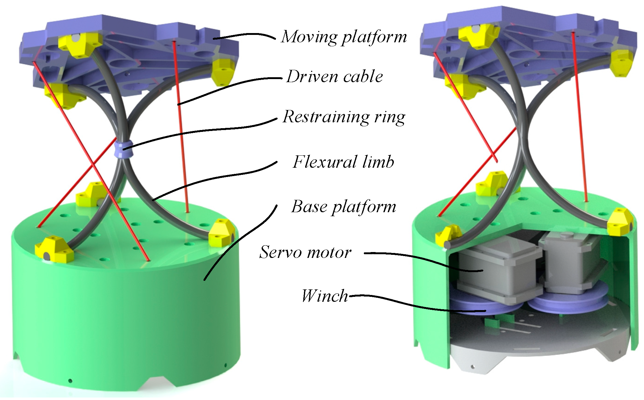
Section 2 introduces the novel compliant mechanism and its structure. Section 3 introduces the theoretical models used in analyzing compliant rods, and discusses the mobility of the novel mechanism. In Section 4, the mechanism is simplified to a rigid model, and kinematic variables are calculated based on the simplified model. Next, the singularity is discussed with force analysis, and the workspace without singularity positions. Finally, a prototype is manufactured and used to verify the mobility analysis and simplified model.

2. Design of the 3R Parallel Compliant Mechanism

In this section, the construction of the novel 3R parallel compliant mechanism prototype structure and its analysis model will be proposed.

2.1. CAD Model

The basic design concept of the novel mechanism is illustrated in Figure 1. The prototype comprises a moving platform, a base, three flexible bars, and three drive cables. Both the moving platform and the base are designed as equilateral circles. The ends of each compliant rod are fixed at the edge of the moving platform and the base, respectively. The tangential direction of the rod’s end is parallel to the moving platform. The three compliant rods are connected at their midpoint by a restraining ring, and the tangential directions at the rods’ midpoint are identical to each other. One end of the drive cable is fixed to the edge of the moving platform, and the other end is fastened to the winch through a guide hole at the base’s edge. A servo motor drives the winch to rotate, and changes in the length of the drive cables result in the movement of the moving platform.

2.2. Mechanism Analysis Model

To analyze the novel mechanism’s movement characteristics, the position and posture of the mechanism will be calculated for any input parameter (three driven cables’ length li i = 1, 2, 3). As shown in Figure 2, the base coordinate is established as follows: the origin point is set at the restraining ring’s center, and X-axis is in the direction from the origin point to the middle point of line segment A1B1. Z-axis is in the direction from the base platform’s center to the moving platform’s center, and Y-axis is determined using the right-hand rule. Three vertices of the moving platform are defined as A1, A2 and A3, the same as the base platform’ vertices to B1, B2 and B3. The length of driven cable from B1 to A1 is defined as l1, the same as l2 and l3.
Next, force analysis will be discussed, which is the hardest part in calculating a compliant mechanism’s kinematics. To analyze the force in the mechanism, the mechanism is separated into the upper part and lower part. The upper part (shown in Figure 2b) contains the moving platform and compliant rods’ segments from the constraining ring to the moving platform, and the remaining parts belong to the lower part (shown in Figure 2d). In analyzing a compliant rod in the upper part, one rod’s end is fixed at the origin point, and the another end exerts forces form the moving platform pfAi and driven cable fi (i = 1, 2, 3), as in the lower part. As mentioned in Section 2.1, the moving platform and the base platform have the same structure dimension. When the mechanism is rotated along any axis in X-Y plane at 180 degrees, the mechanism will keep the same shape and position. This means that the upper part and lower part can be replaced by each other. Thus, the force pFA1 has equal numerical value and opposite direction compared to pFB1, the same as pFA2 and pFA3.
F Ai p + F Bi p = 0 ( i = 1 , 2 , 3 )
Since the cables can only bear tension, the force Fl1 is coincident with cable direction, the same as Fl2 and Fl3.
F l i × A i B i ¯ = 0 ( i = 1 , 2 , 3 )
For the moving platform, this just bears the moment of the force from three compliant rods at the rods’ ends. When the system reaches equilibrium, the amount of external force in the moving platform is zero.
i = 1 3 F Ai p = i = 1 3 F Bi p = 0
According to the geometric constraint, the direction of the rods’ ends is collinear to the platform’s triangle midline, and the direction of the other end is collinear to the Z-axis:
d 3 A 1 ( 1 ) × ( A 1 A 2 ¯ + A 1 A 3 ¯ ) = d 3 A 2 ( 1 ) × ( A 1 A 2 ¯ + A 2 A 3 ¯ ) = d 3 A 3 ( 1 ) × ( A 3 A 2 ¯ + A 1 A 3 ¯ ) = 0 d 3 B 1 ( 1 ) × ( B 1 B 2 ¯ + B 1 B 3 ¯ ) = d 3 B 2 ( 1 ) × ( B 1 B 2 ¯ + B 2 B 3 ¯ ) = d 3 B 3 ( 1 ) × ( B 3 B 2 ¯ + B 1 B 3 ¯ ) = 0
where d3ij (i = A, B; j = 1, 2, 3) is the normal of the rods’ cross-section, as explained in Section 3.2.
According to the structure, the length between the rods’ ends is equal to the triangle’s side length:
A 1 A 2 ¯ = A 2 A 3 ¯ = A 3 A 1 ¯ = 3 r a B 1 B 2 ¯ = B 2 B 3 ¯ = B 3 B 1 ¯ = 3 r a
Assuming there is a function between forces and position at the compliant rod’s end:
{ x , y , z , q 1 , q 2 , q 3 , q 4 } = F f ( F , M )
According to the lengths of driven cables:
A i B i ¯ = l i ( i = 1 , 2 , 3 )
By solving Equations (1)–(7) above, the moving platform’s position and pose can be obtained. However, the relationship between the compliant rod’s deformation and force is unknown. On the other hand, the equations are nonlinear and huge, and almost cannot be solved with analytical solutions. To solve these problems, three methods will be applied here and introduced in next section.

3. Theoretical Model

In this section, three methods will be introduced to analyze the mechanism’s movement characteristics. At first, the Cosserat rod model will be applied to the analysis of the compliant rod. The relationship between force and deformation of a compliant rod will be investigated with the Cosserat rod model and Lagrangian dynamics equation. Next, the relationship will be trained as a neural network, and the neural network will be used to calculate the mechanism’s kinematics. To solve a large number of nonlinear equations in the mechanism’s kinematics, a chaos-enhanced accelerated particle swarm optimization method will be used.

3.1. Method 1: Cosserat Rod Model

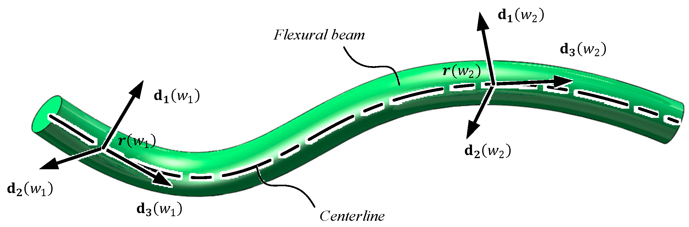
This section provides a brief introduction to the Cosserat rod model of elastic rods. An elastic rod can be visualized as a long thin deformable body. If a rod’s length is much greater than its radius, the rod’s continuous configuration can be characterized by the centerline r(w) = {rx(w), ry(w), rz(w)}T, where r(w) assigns a position in space to each line parameter value w ∈ [0, 1]. An orthonormal frame with basis vectors {d1(w), d2(w), d3(w)} is attached to every point on the curve, such that d1 and d2 span the plane of the rod’s cross-section, and d3 is the normal to the cross-section (as shown in Figure 3).
To relate the directions di to the reference frame, quaternions are chosen as a representation of rotation. Quaternions can be present as a quadruple q = {q1, q2, q3, q4}T with qiR. Only unit quaternions represent pure rotations, thus the qi is not independent but coupled by the constraint ‖q‖ = 1. The directions di in terms of the quaternion q are given by:
d 1 = { q 1 2 q 2 2 q 3 2 + q 4 2 , 2 ( q 1 q 2 + q 3 q 4 ) , 2 ( q 1 q 3 q 2 q 4 ) } T d 2 = { 2 ( q 1 q 2 q 3 q 4 ) , q 1 2 + q 2 2 q 3 2 + q 4 2 , 2 ( q 2 q 3 + q 1 q 4 ) } T d 3 = { 2 ( q 1 q 3 + q 2 q 4 ) , 2 ( q 2 q 3 q 1 q 4 ) , q 1 2 q 2 2 + q 3 2 + q 4 2 } T
For elastic rods, the potential energy consists of three parts, namely the energy versus the stretch deformation, energy Vb of the bending deformation, and energy Vt of the torsional deformation. However, the bending deformation and torsional deformation are similar in expression, and can be integrated to Vb,t. The three energies are given as:
V s = 1 2 0 1 K s ( r 1 ) 2 d w V b , t = 1 2 0 1 k = 1 3 K k ( 2 q 2 B k q q u ^ k ) 2 d w
where Ks = Esπrr2 is the stretching stiffness; Es is the stretch modulus; the ûk conform to the intrinsic bending and torsion of the rod; Kk is the stiffness tensor (K1 = K2 = 0.25 Eπrr2, K3 = 0.5 Gπrr2); E is the Young’s modulus governing the bending resistance; G is the shear modulus governing the torsional resistance; and rr is the radius of the rod’s cross-section.
The dynamic equilibrium configuration of an elastic rod is characterized as a critical point of the Lagrangian. Details can be found in Goldstein [32].
d d t T g ˙ i T g i + V g i + D g ˙ i + λ C p g i + μ C q g i = 0 1 F e d w D = 1 2 0 1 γ t r ( r ˙ r ) r 2 r ( r ˙ r ) r 2 d w + 1 2 0 1 γ r 2 B k 0 q q ˙ q 2 2 B k 0 q q ˙ q 2 d w C p = r r d 3 = 0 C q = q 2 1 = 0
where the gi∈{rx, ry, rz, q1, q2, q3, q4} are coordinates and Fe are external forces and torques; T and V = vs. + Vb + Vt are the kinetic energy and the potential energy of the system; D is the total dissipation energy; γt is the translational internal friction coefficient; γr is the rotational internal friction coefficient; Cp and Cq are holonomic constraints; λ and μ are Lagrangian multipliers; Bk and Bk0 are a constant skew-symmetric matrix; r’ is the tangent vector at point r; r ˙ ′ is the derivative of r′.
B 1 = 0 0 0 1 0 0 1 0 0 1 0 0 1 0 0 0 , B 2 = 0 0 1 0 0 0 0 1 1 0 0 0 0 1 0 0 , B 3 = 0 1 0 0 1 0 0 0 0 0 0 1 0 0 1 0 B 1 0 = 0 0 0 1 0 0 1 0 0 1 0 0 1 0 0 0 , B 2 0 = 0 0 1 0 0 0 0 1 1 0 0 0 0 1 0 0 , B 3 0 = 0 1 0 0 1 0 0 0 0 0 0 1 0 0 1 0

3.2. Method 2: Back-Propagation Neural Network

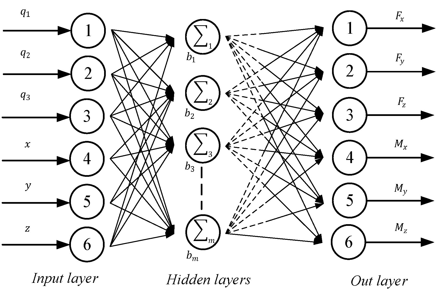
The back-propagation (BP) network is a widely used multi-layer feed-forward network with error inverse propagation. It is generated using the BP algorithm, which is a type of supervised learning algorithm. The BP algorithm continuously calculates the network’s weights and the error’s trend in the direction that minimizes the error. By doing so, it gradually reduces the error until the sum of squares of errors is minimal. The weights and the error’s trend are positively correlated with the network’s errors and are transmitted in reverse to every layer. The BP network can learn and store numerous input–output mapping relationships without a mathematical expression. It can be used to map the relationship between forces and the position and direction at a compliant rod’s end.
A BP network consists of an input layer, an output layer, and multiple hidden layers. In this study, positions and quaternions of a compliant rod are taken as the input layer, and the forces at the rod’s end are taken as the output layer. This BP network’s structure is shown in Figure 4, and can replace the function Ff in Equation (6). To train the neural network, 6.4 × 10⁷ sets of data are calculated and used as the samples.

3.3. Method 3: Chaos-Enhanced Accelerated Particle Swarm Optimization Method

Kennedy and Eberhart developed the standard Particle Swarm Optimization (PSO) in 1995. Extensive studies have demonstrated that PSO is highly efficient for optimizing many problems. However, for highly multimodal problems, it may suffer from premature convergence. The standard PSO uses g (the current global best) and x (the individual best) to increase the diversity in quality solutions. To simplify the algorithm and accelerate convergence, the global best can be used exclusively. In 2008, accelerated particle swarm optimization (APSO) [33] was proposed, which generates the velocity vector using a simpler formula.
v i t + 1 = v i t + α r r a n d o m ( t ) + β ( g * x i t )
where rrandom is drawn from N (0,1).
During each iteration, the particle’s position is updated by
x i t + 1 = x i t + v i t + 1 Δ t
The randomization term αr allows the system to escape local optima, and r can be solved by a probability distribution. Typically, a value of β ranging from 0.2 to 0.7 is adequate for most situations. Another enhancement to APSO involves reducing randomness as iterations progress. This can be achieved using the follow function:
α = δ t
where 0 < δ < 1 is an annealing-like parameter whose value can be taken as 0.7 to 0.9 for most applications; t is the t-th iteration.
There is no requirement to maintain a constant value of β in standard APSO. However, a varying β may provide advantages and lead to faster convergence of the algorithm. Since all chaotic maps are normalized, a chaos-enhanced APSO (known as chaotic APSO) uses the chaotic map to tune the parameter β. In [34], after comparing various chaotic APSO variants, the sinusoidal map is deemed the best chaotic APSO, and is expressed as follows:
β k + 1 = a β k 2 sin ( π β k )

3.4. Numerical Computation

In this section, all these three methods will be integrated. There are two steps in this integration. The first is to analyze a single compliant rod with the Cosserat rod model and BP network. The second is to build the compliant mechanism’s kinematical model.
The purpose of the first step is to establish the relationship between forces, positions and quaternion of a compliant rod. First, the rod will be simplified to a Cosserat rod model. By solving the Lagrange dynamic equations, the rod’s position and quaternion can be calculated under forces. In addition, all the material parameters for the compliant rod are shown in Table 1. To facilitate the solution of the motion’s equations, the rod is discretized into elements. First, the centerline of the rod is expressed as a chain of N nodes ri, i ∈ [1, N]. The centerline elements ri+1ri may differ in size. The orientations of the centerline elements are represented by quaternions qj, j ∈ [1, N − 1], as illustrated in Figure 2. The discrete spatial derivative ri′ of the centerline and qj′ are obtained as
r i = r i + 1 r i r i + 1 r i q j q j + 1 q j r j + 1 r j
Next, a large number of the rod’s positions and quaternions can be calculated as samples in the training BP network. Taking the positions and quaternions as the input parameters and the forces and moments as the output parameters, the BP network is trained with 10 hidden neurons and the Levenberg–Marquardt algorithm.
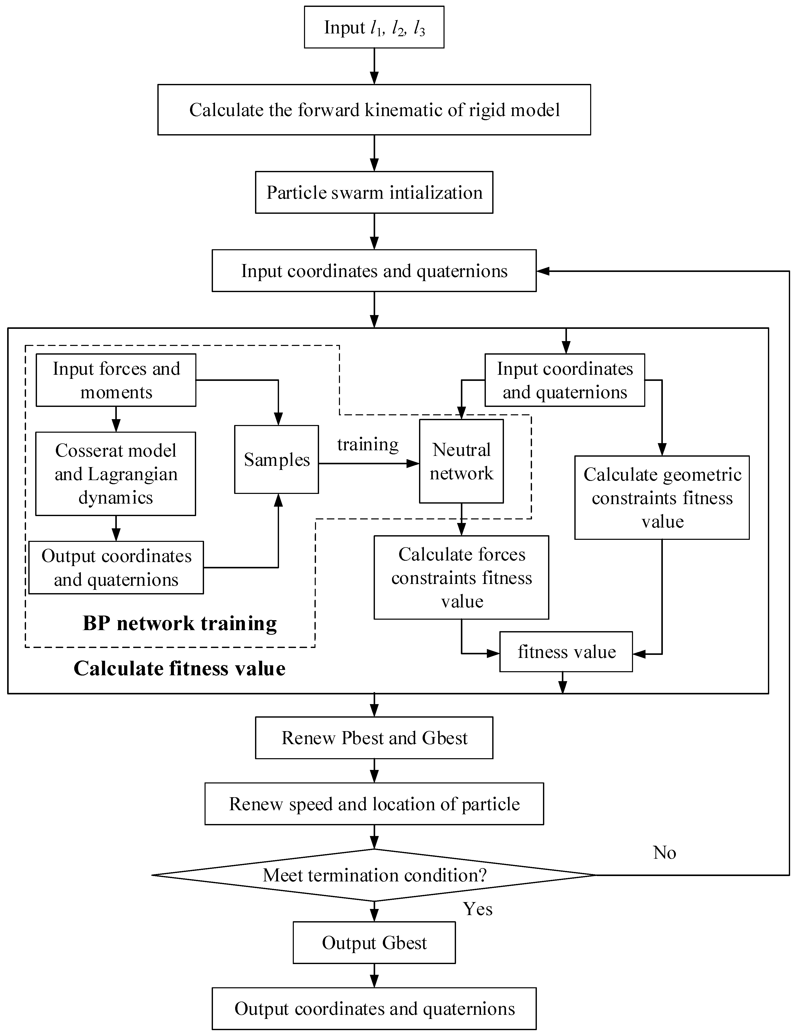
The second step is to build the compliant mechanism’s kinematical model. The model is introduced in Section 2.2. However, as it is hard to solve these equations with an analytical solution, the chaos-enhanced accelerated particle swarm optimization method is used here. As shown in Figure 5, the numerical computation can be separated into serval steps:
(a) taking the mechanism as a rigid mechanism, the position and quaternions can be calculated. The result can be taken as the initial value. Next, all particle swarms can be initialed.
(b) calculating the fitness value.
(c) renewing the Pbest, Gbest and particles’ speed and location.
(d) judging the termination condition. If the Gbest meets the termination condition, output the Gbest; if not, come back to step (a).

3.5. Results and Summary

For numerical computation, the radii of the moving platform and base platform is set as 65 mm. The range of the driven cable’s length is set to be 65 mm–185 mm. To reduce the calculation amount and ensure the result’s reliability, 124 sets inputs are chosen randomly from the range of the driven cable’s length.
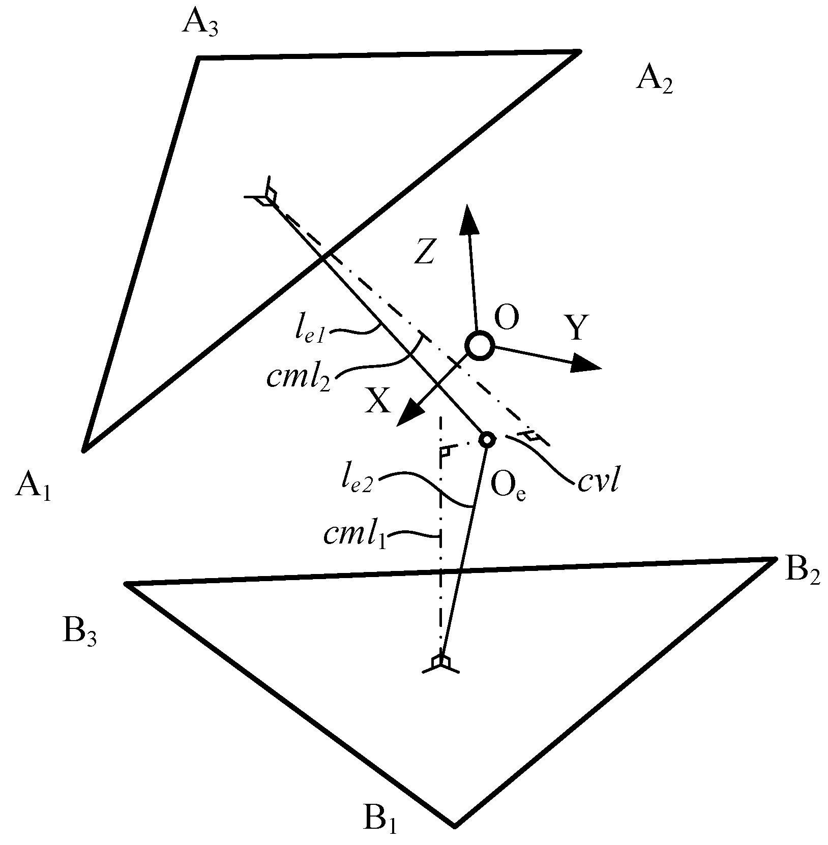
Next, all these positions will be analyzed. The relative motion between a moving platform and base platform will be investigated. According to the moving platform and base platform positions, the relative rotating center (RRC) and the relative rotating radius (RRR) will be defined here. As shown in Figure 6, cml1 is the normal line of the moving platform via the moving platform’s center point OA, the same as cml2 to base platform. Next, the common vertical line of cml1 and cml2 could be found, and the middle point of common vertical line is set as Oe. Point Oe is approximately seen as the relative rotational center. Next, the distance between Oe and the moving platform’s center point OA is approximately seen as its relative rotational radii le1, the same as le2 to the base platform. The mean of le1 and le2 are seen as the mechanism’s RRR.
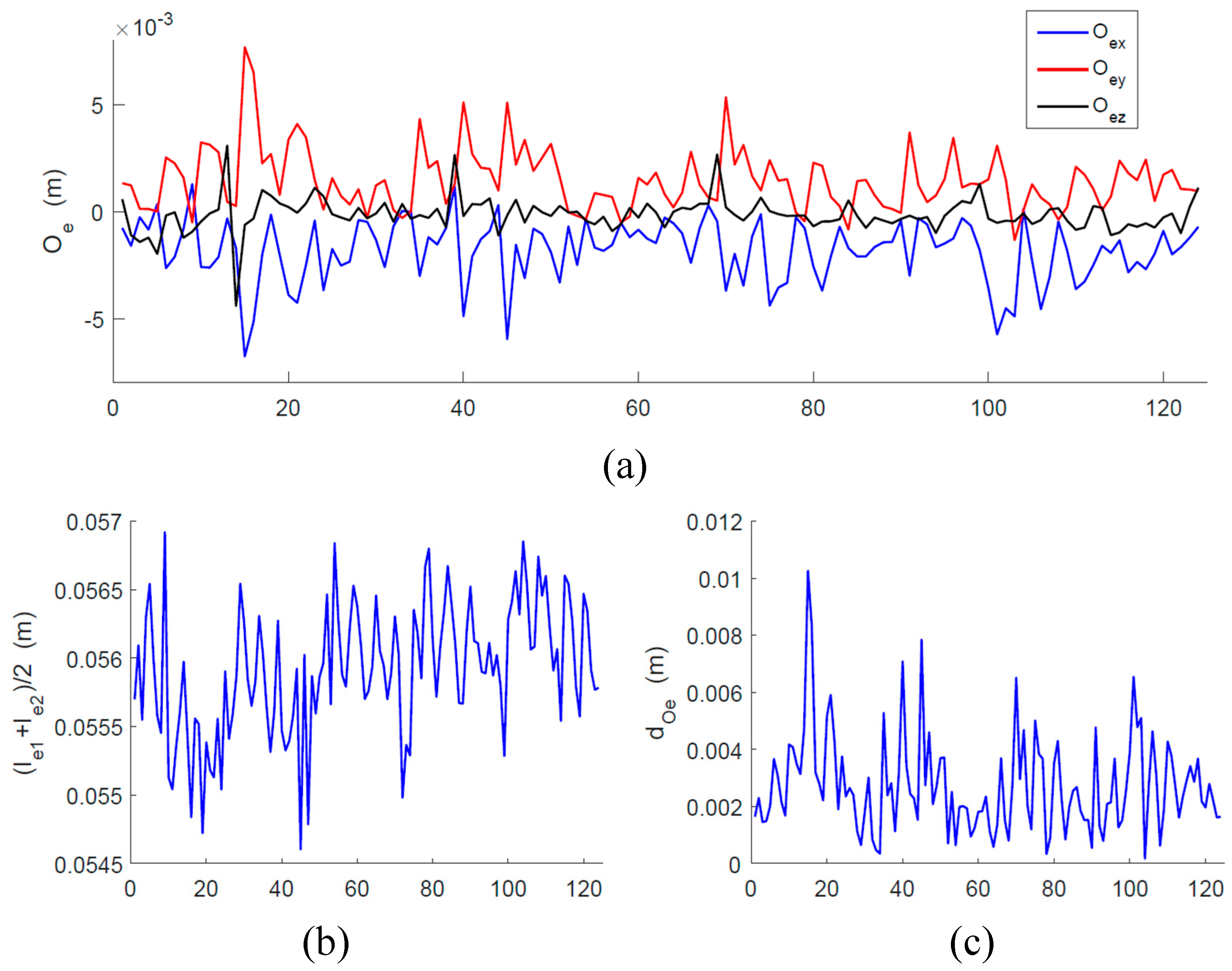
According to the position results, a set of RRC and RRR can be calculated. The results are shown in Figure 7. From Figure 7c, the RRC is close to the origin point O, and the mean distance is 2.7 mm. On the other hand, the RRR ranges from 54 mm to 57 mm, and the mean is 56 mm. It is obvious that 2.7 is far less than 56 mm, which means that origin point O could be taken as the mechanism’s RRC. In addition, the RRR can be seen as a constant. A constant rotate radius and a fixed rotational center means that the moving platform and base platform move along a spherical surface. In summary, the moving platform has three spatial rotational degrees of freedom.

4. Kinematics Analysis of 3R Parallel Compliant Mechanism

From the conclusion in 
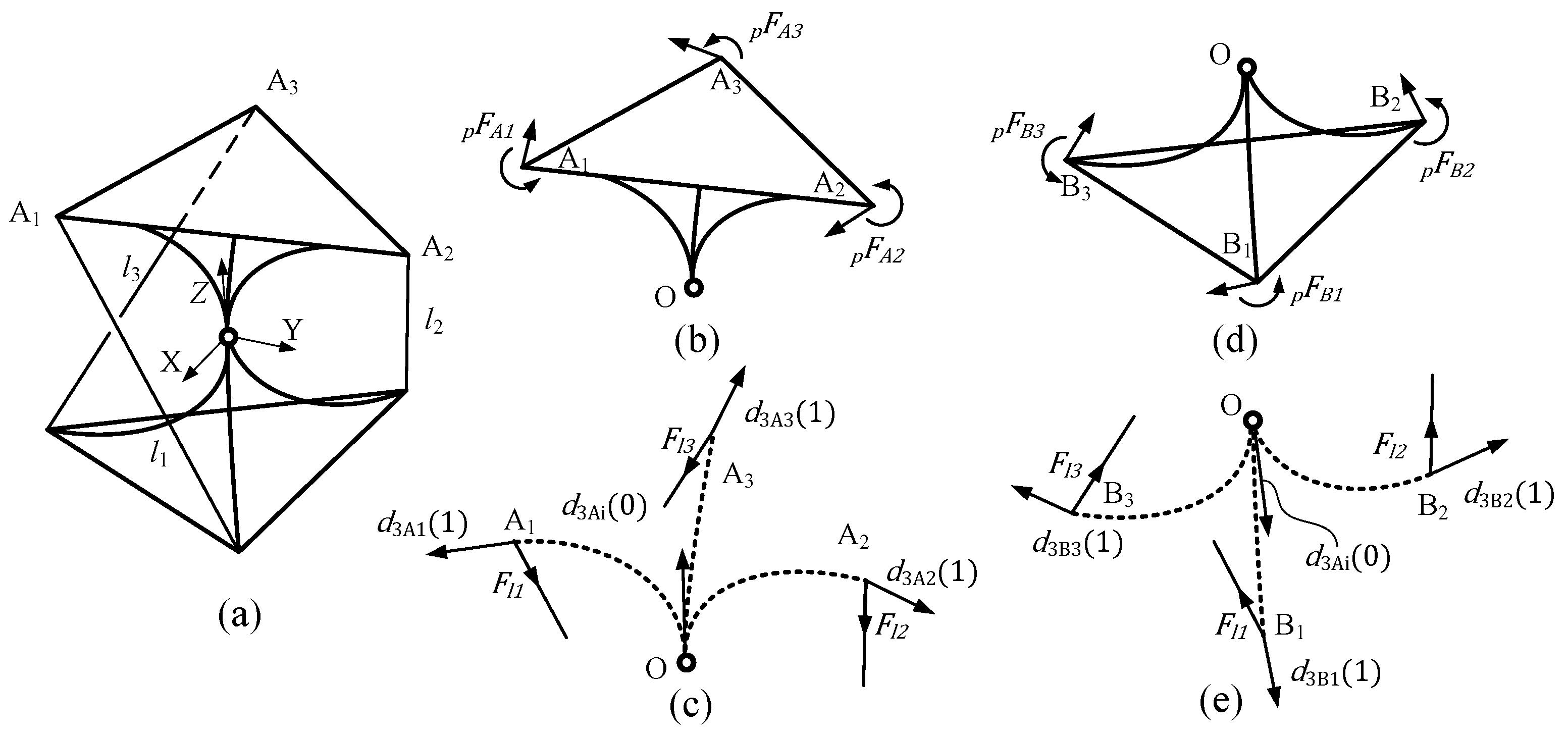
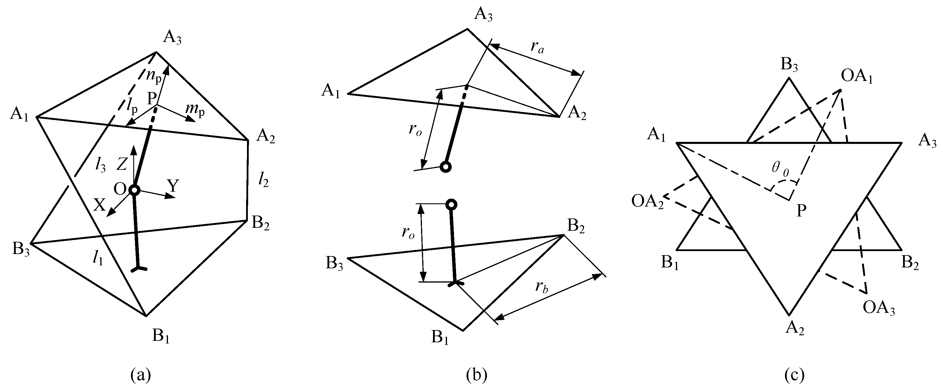
Section 3.5, the novel compliant mechanism is a device whose moving platform can rotate around the center point in any direction. Thus, it can be considered to be a rigid parallel mechanism with three rotational degrees of freedom. As shown in Fig.8, three flexural limbs are replaced by a spatial ball hinge at a center point. On the other hand, the driven cable can only bear the tension. That means the cable can just drive the moving platform rotate counterclockwise along the Z-axis. To drive the moving platform to rotate clockwise at the initial position, there must be a pre-rotation at the initial position. As shown in Figure 8c, the position OA1OA2OA3 is the moving platform in assembly-complete state without pre-rotation. Next, a pre-rotation is applied to the mechanism. Then, the mechanism reaches the initial position A1A2A3 with a counterclockwise degree θ0.

4.1. Direct Kinematics

The direct kinematics analysis of a parallel mechanism aims to calculate moving platform attitude angles and positions according to given joint variables. For the novel mechanism, the three driven cables’ lengths li (I = 1, 2, 3) are joint variables, and the three attitude angles are the moving platform’s pose. In this study, Z-Y-X Euler angles are applied to express the moving platform’s pose, as the sensor in the experiment used it. The Z-Y-X Euler angles mean that the moving platform rotates θz degrees along the Z-axis of the fixed frame first, acquiring a new frame X′Y′Z′. Then, the moving platform rotates θy degrees along the Y′-axis of the new frame X′Y′Z′, acquiring another new frame X″Y″Z″. After that, the moving platform rotates θx degrees along X″-axis of the new frame X″Y″Z″. Next, the rotation matrix of the moving platform can be expressed as follows.
R = C y C z C y S z S y C z S x S y C x S z C x C z + S x S y S z C y S x C x C z S y + S x S z C z S x + C x S y S z C x C y
where Ci and Si represent cos(θi) and sin(θi), and i = x, y, z.
At the initial position, the vertexes’ coordinates of the moving platform and base platform can be expressed as follows.
A 1 , 0 = 1 2 r a , 3 2 r a , r o T , A 2 , 0 = 1 2 r a , 3 2 r a , r o T , A 3 , 0 = r a , 0 , r o T B 1 = 1 2 r b , 3 2 r b , r o T , B 2 = r b , 0 , r o T , B 3 = 1 2 r b , 3 2 r b , r o T
Then, the vertexes’ coordinate of the moving platform at any position can be written as follows.
A i = R A i , 0 ( i = 1 , 2 , 3 )
According to the given driven cables’ lengths li, forward kinematics equations can be obtained.
l i = A i B i ¯ ( i = 1 , 2 , 3 )
By solving Equation (19), three Euler angles can be obtained.

4.2. Inverse Kinematics

The inverse kinematics of the novel mechanism aims to solve the three driven cable’s lengths according to a given moving platform pose. According to Equations (16)–(19), the inverse kinematics can be solved.
l i = ( R A i , 0 B i ) ( R A i , 0 B i ) ( i = 1 , 2 , 3 )

4.3. Results and Summary

A mechanism is driven by actuators to move. When a mechanism experiences changes in its kinematical or dynamic performance at certain positions, it may become stuck in dead-point positions, lose balance stability, or alter its degree of freedom. Consequently, the mechanism cannot transfer movements or be controlled properly. These positions are known as singularities. In the case of a novel mechanism, the movement of the moving platform depends on compliant rods and driven cables. Thus, the mechanism will only encounter singularity positions when the deformation of the compliant rods disappears or the tension in the driven cables disappears.

4.3.1. Compliant Rods’ Deformation Disappearance

Compliant rods’ deformation includes bending, stretching, and twisting. In this mechanism, the compliant rods mainly bear radial forces, so stretching will not be discussed here. The key points are bending and twisting deformation. When rod bending disappears, rods will recover to become straight rods. However, whatever position the moving platform is in, the compliant rod will always bend. As a result, the rod bending will not disappear.
For rod twisting deformation, when the mechanism is at initial position, there is a pre-rotation along the Z-axis. When the twisting deformation disappeared, the mechanism’s pre-rotation will disappear. Thus, when the moving platform’s rotation angle along the Z-axis clockwise is bigger than θ0, the mechanism is in singularity positions.
θ z θ 0

4.3.2. Driven Cables’ Tension Disappearance

Considering that cables only can bear tension, when the driven cables’ tension disappears, the moving platform will lose the control along with the power from driven cables. Thus, the mechanism is in a singularity position.
When the three driven cables’ length are given, the position and quaternion can be calculated according to Section 4.1. Next, the forces at the rods’ ends can be calculated from Section 3.1, and the driven cable’s force Fli can be obtained too.
F l i + F Ai p = F f ( A i , q A i ) ( i = 1 , 2 , 3 )
When the directions of cables’ force were reverse to vector A i B i ¯ , the mechanism is in singularity positions.
F l i A i B i ¯ 0 ( i = 1 , 2 , 3 )

4.4. Workspace

In this section, the parasitic motion workspace and the reachability of the novel mechanism are obtained based on forward position analysis and singularity analysis. The key points in analyzing the workspace are the mechanism’s kinematical constraints and singularity. The kinematical constraints include action range and physical joint range.
The actuator’s range limits the mechanism’s workspace. Because of the actuator’s physical structure, its range is usually between a minimum value and a maximum value. The corresponding actuator’s constraint condition can be expressed as follows:
80 m m l i 150 m m ( i = 1 , 2 , 3 )
Physical joints also limit the mechanism’s range of motion. As mentioned in Section 3.5, the compliant rods are equivalently replaced by a ball hinge joint. However, a ball hinge joint’s range is limited by its physical structure. For this mechanism, the moving platform and base platform have the same structure size, so the maximum angle between these two platforms is 90 degrees. Thus, the angle between the moving platform’s normal and Z-axis should be less then 90 degrees. According to the rotation matrix, this constraint can be present as
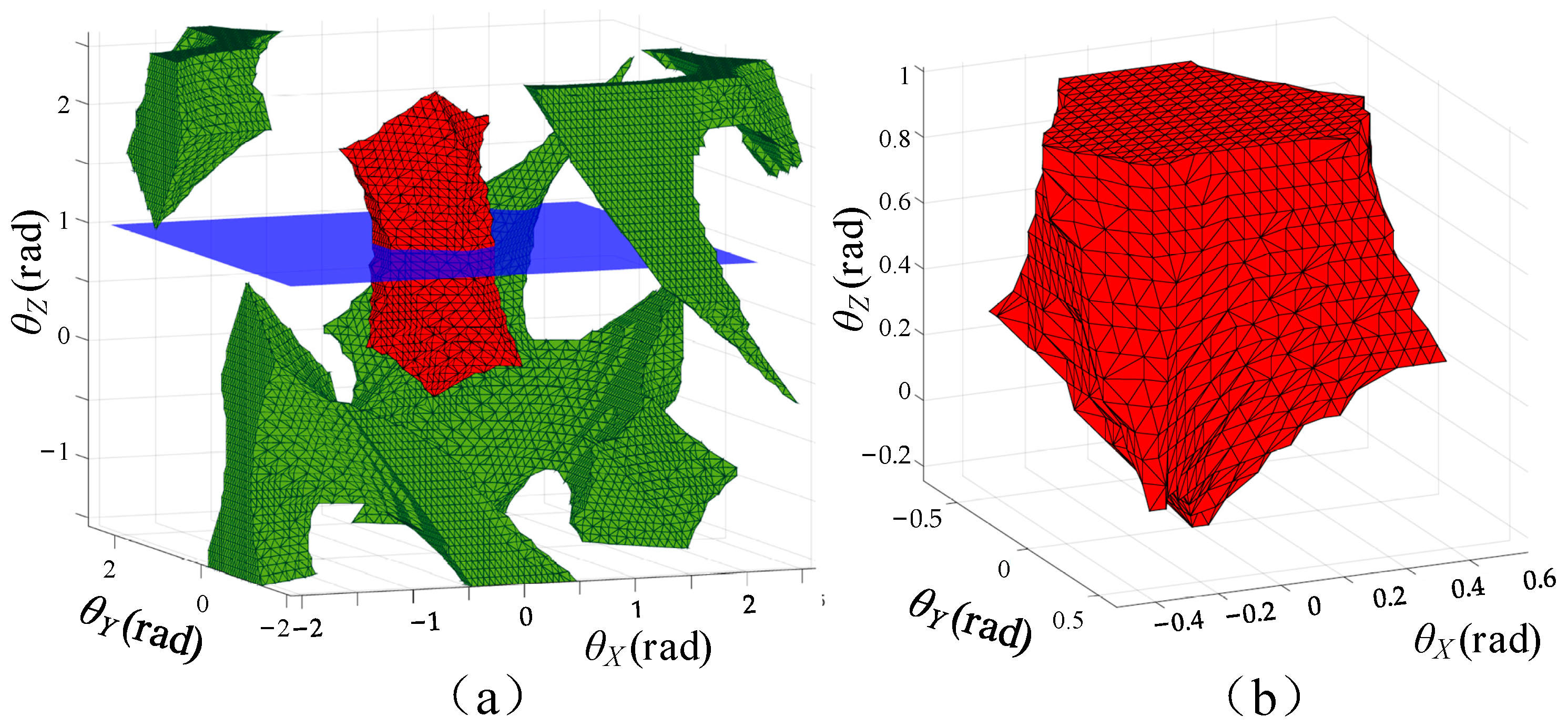
( R 0 , 0 , 1 T ) 0 , 0 , 1 T 0
According to Section 4.3, the mechanism has two kinds of singularity position. The first depends on the pre-rotation angle. When the prototype is manufactured, the pre-rotation angle θ0 is set as 60 degrees. The second singularity position is related to the mechanism’s forward kinematic and force analysis in Section 2.2.
Figure 9a shows the mechanism’s workspace with singularity positions. The blue plane is the border of the pre-rotation angle, and the green parts are the positions of that mechanism’s driven cable without tension. After excluding singularities, the mechanism’s final workspace is shown in Figure 9b.

5. Validation and Results

To verify the simplified model and improve the algorithm’s accuracy and stability, two group experiments are designed in this section. An angle sensor is fixed on the moving platform to measure its Z-Y-X Euler angles.

5.1. Experimental Design

These two group experiments are designed to test the mechanism’s forward and inverse kinematics model. In the forward kinematics experiment, a set of input parameters are designed and input to the prototype and simulation. Next, the output Euler angles from the prototype and simulation will be recorded. In the inverse kinematics experiment, a set of moving platform movement trajectories is designed, and the input parameters are calculated according to the simplified model. Next, the input parameters are input to the prototype, and the output angles of the moving platform are recorded.

5.2. Experimental Setup

The experimental devices (shown in Figure 10) include a novel mechanism’s prototype, an angle sensor and an analysis system. The prototype applies three high-performance actuators (dynamixel mx64t). The actuators whose maximum output torque is 5 Nm can achieve 360° rotation. The angle sensor (jy901) weighs about 50 g and integrates a nine-axes accelerometer and dynamic Kalman filter, and can output angles, angular velocities and angular accelerations in three axes. The analysis system is a high-performance workstation with Intel i7-6850 CPU, Amd w5100 graphic card. Communication with the prototype and the sensor is carried out using Matlab installed on a workstation. Two serial ports are used in Matlab. One sends input parameters to the prototype with RS485 protocol. The other one receives angle data from the sensor with the RS232 protocol. The moving platform of the prototype weighs about 95 g.
In the forward kinematics experiment, three sets of input parameters (shown in Figure 11a) are designed. The first set is designed with only one actuator driven along a straight line. The second set is driven by two actuators along the same straight line. In the third set, three actuators move along a straight line, but one of them moves in the opposite direction. The workstation sends these parameters into the prototype and drives the prototype movement. Next, the Euler angle data from the angle sensor is recorded.
In an inverse kinematics experiment, three sets of moving platform movement trajectories (shown in Figure 11b) are designed. In these three trajectories, the moving platform rotates along three axes. Next, the input parameters are calculated with the simplified model, and be sent to the prototype. Then, the moving platform’s angles are recorded from the sensor.

5.3. Experiment Results and Analysis

By comparing the recorded data from the sensor and given the movement trajectory, the simplified model and improved algorithm accuracy and stability in inverse kinematics is discussed. As shown in Figure 12, the recorded data are drawn as curves. All these curves are made up of three segments. The first one is from the beginning to 602 ms, the second one is from 602 ms to 1204 ms, and the last one is from 1204 ms to 1806 ms.
In Figure 12a, the experiment data almost coincides with the simulation data in the X- and Y-axes, showing the same curve trend. However, there are still some differences, as the experimental data’s amplitude is lower than the simulation data. Two main reasons explain the difference. First, plastic deformation reduces the rotation angle, and deviations occur mainly in positions with large angles. Second, deviations also occur at inflection points, especially at junctions between two segments. The actuator’s acceleration is not continuous at inflection points, causing a shiver in the moving platform and magnifying the sensor’s error. In the Z-axis, the experimental data shows the same trend as the simulation data, but its deviation is more obvious than in the X- and Y-axes. This is mainly due to the sensor, which measures the Z-axis angle differently from the X- and Y-axes. The angle in the Z-axis is obtained by measuring the Earth’s magnetic induction line, which is easily influenced by external factors, such as the electrical motor’s magnetic field.
In Figure 12b, the experiment data in the inverse kinematic experiment almost coincides with the simulation data for the three axes, and there are still errors because of the plastic deformation, inflection points, and external interferences. However, the errors are lower than in the forward kinematic experiment. This means the simplified model performs better in inverse kinematic, and is good for controlling the mechanism.
In summary, the experiment results tally with the simulation results in both forward and inverse kinematics. The experiment results not only verify the simplified model’s accuracy, but also prove that the novel mechanism has three rotational degrees of freedom.

6. Conclusions

In this paper, a novel compliant mechanism with three rotational degrees of freedom is proposed. The compliant rods are simulated with Cosserat rod models, and the mechanism is analyzed with a back-propagation neural network and chaos-enhanced accelerated particle swarm optimization method. Next, the mechanism’s mobility is verified by numerical analysis, and the mechanism is simplified into a rigid mechanism whose compliant rods are replaced by a spatial ball hinge. With the simplified model, the mechanism’s forward and inverse kinematics can be calculated more effectively. In addition, with force analysis, the mechanism’s singularity is calculated, and the workspace without singularity positions is obtained. Finally, experiments with a prototype verify the mobility analysis and simplified model.

Author Contributions

Conceptualization, L.P. and J.W.Z.; methodology, L.P. and H.T.; software, J.W.Z. and H.T.; validation, L.P., J.W.Z. and D.Z.; formal analysis, L.P.; writing—original draft preparation, L.P. and J.W.Z.; writing—review and editing, D.Z. and H.T. All authors have read and agreed to the published version of the manuscript.

Funding

This research received no external funding.

Data Availability Statement

Data sharing is not applicable to this article.

Conflicts of Interest

The authors declare no conflict of interest.

References

  1. Schitter, G.; Thurner, P.J.; Hansma, P.K. Design and input-shaping control of a novel scanner for high-speed atomic force microscopy. Mechatronics 2008, 18, 282–288. [Google Scholar] [CrossRef]
  2. Kim, D.; Lee, D.Y.; Gweon, D.G. A new nano-accuracy AFM system for minimizing Abbe errors and the evaluation of its measuring uncertainty. Ultramicroscopy 2007, 107, 322–328. [Google Scholar] [CrossRef]
  3. Pham, M.T.; Yeo, S.H.; Teo, T.J.; Wang, P.; Nai, M.L.S. A Decoupled 6-DOF Compliant Parallel Mechanism with Optimized Dynamic Characteristics Using Cellular Structure. Machines 2021, 9, 5. [Google Scholar] [CrossRef]
  4. Alblalaihid, K.; Lawes, S.; Kinnell, P. Variable stiffness probing systems for micro-coordinate measuring machines. Precis. Eng. 2016, 43, 262–269. [Google Scholar] [CrossRef] [Green Version]
  5. Jin, Z.; Gao, F.; Zhang, X. Design and analysis of a novel isotropic six-component force/torque sensor. Sens. Actuators A Phys. 2003, 109, 17–20. [Google Scholar]
  6. Hao, G.; Murphy, M.; Luo, X. Development of a compliant mechanism-based compact three-axis force sensor for high-precision manufacturing. In Proceedings of the ASME 2015 International Design Engineering Technical Conferences & Computers and Information in Engineering Conference (IDETC/CIE 2015), Boston, MA, USA, 2–5 August 2015. [Google Scholar]
  7. Hansen, B.J.; Carron, C.J.; Jensen, B.; Hawkins, A.; Schultz, S. Plastic latching accelerometer based on bistable compliant mechanisms. Smart Mater. Struct. 2007, 16, 1967. [Google Scholar] [CrossRef]
  8. Gao, Z.; Zhang, D. Design, analysis and fabrication of a multidimensional acceleration sensor based on fully decoupled compliant parallel mechanism. Sens. Actuators A Phys. 2010, 163, 418–427. [Google Scholar] [CrossRef]
  9. Sung, E.; Slocum, A.H.; Ma, R.; Bean, J.F.; Culpepper, M.L. Design of an ankle rehabilitation device using compliant mechanisms. J. Med. Devices 2011, 5, 011001. [Google Scholar] [CrossRef] [Green Version]
  10. Chen, G.; Zhang, S. Fully-compliant statically-balanced mechanisms without prestressing assembly: Concepts and case studies. Mech. Sci. 2011, 2, 169–174. [Google Scholar] [CrossRef] [Green Version]
  11. Awtar, S.; Trutna, T.T.; Nielsen, J.M.; Abani, R.; Geiger, J. FlexDex™: A minimally invasive surgical tool with enhanced dexterity and intuitive control. J. Med. Devices 2010, 4, 035003. [Google Scholar] [CrossRef]
  12. Liew, L.A.; Tuantranont, A.; Bright, V. Modeling of thermal actuation in a bulk-micromachined CMOS micromirror. Microelectron. J. 2000, 31, 791–801. [Google Scholar] [CrossRef]
  13. Olfatnia, M.; Cui, L.; Chopra, P.; Awtar, S. Large range dual-axis micro-stage driven by electrostatic comb-drive actuators. J. Micromechanics Microengineering 2013, 23, 105008. [Google Scholar] [CrossRef] [Green Version]
  14. Olfatnia, M.; Sood, S.; Gorman, J.J.; Awtar, S. Large stroke electrostatic comb-drive actuators enabled by a novel flexure mechanism. J. Microelectromechanical Syst. 2013, 22, 483–494. [Google Scholar] [CrossRef]
  15. Aten, Q.T.; Jensen, B.D.; Burnett, S.H.; Howell, L.L. A self-reconfiguring metamorphic nanoinjector for injection into mouse zygotes. Rev. Sci. Instrum. 2014, 85, 055005. [Google Scholar] [CrossRef]
  16. Fowler, R.; Howell, L.; Magleby, S. Compliant space mechanisms: A new frontier for compliant mechanisms. Mech. Sci. 2011, 2, 205–215. [Google Scholar] [CrossRef] [Green Version]
  17. Thalmann, E.; Gubler, Q.; Henein, S. Gravity-Compensation Design Approaches for Flexure-Pivot Time Bases. Machines 2022, 10, 580. [Google Scholar] [CrossRef]
  18. MIdha, A. Parametric deflection approximations for end-loaded, large-deflection beams in compliant mechanisms. J. Mech. Des. 1995, 117, 157. [Google Scholar]
  19. Awtar, S.; Slocum, A.H. Constraint-based design of parallel kinematic XY flexure mechanisms. J. Mech. Des. 2007, 129, 816–830. [Google Scholar] [CrossRef]
  20. Awtar, S.; Slocum, A.H.; Sevincer, E. Characteristics of beam-based flexure modules. J. Mech. Des. 2007, 129, 625–639. [Google Scholar] [CrossRef] [Green Version]
  21. Hao, G.; Kong, X.; Reuben, R.L. A nonlinear analysis of spatial compliant parallel modules: Multi-beam modules. Mech. Mach. Theory 2011, 46, 680–706. [Google Scholar] [CrossRef]
  22. Sen, S.; Awtar, S. A closed-form nonlinear model for the constraint characteristics of symmetric spatial beams. J. Mech. Des. 2013, 135, 031003. [Google Scholar] [CrossRef]
  23. Awtar, S.; Sen, S. A generalized constraint model for two-dimensional beam flexures: Nonlinear strain energy formulation. J. Mech. Des. 2010, 132, 081009. [Google Scholar] [CrossRef]
  24. Howell, L.L.; Magleby, S.P.; Olsen, B.M. Handbook of Compliant Mechanisms; John Wiley & Sons: Hoboken, NJ, USA, 2013. [Google Scholar]
  25. Kramer, S.; Saxena, A. A simple and accurate method for determining large deflections in compliant mechanisms subjected to end forces and moments. J. Mech. Des. 1998, 120, 392–400. [Google Scholar]
  26. Midha, A.; Howell, L. Evaluation of equivalent spring stiffness for use in a pseudo-rigid-body model of large deflection compliant mechanisms. ASME Trans. J. Mech. Des. 1996, 118, 126–131. [Google Scholar]
  27. Bilancia, P.; Berselli, G. Design and testing of a monolithic compliant constant force mechanism. Smart Mater. Struct. 2020, 29, 044001. [Google Scholar] [CrossRef]
  28. Venkiteswaran, V.K.; Su, H.J. A parameter optimization framework for determining the pseudo-rigid-body model of cantilever-beams. Precis. Eng. 2015, 40, 46–54. [Google Scholar] [CrossRef]
  29. Bryson, C.E.; Rucker, D.C. Toward parallel continuum manipulators. In Proceedings of the 2014 IEEE International Conference on Robotics and Automation (ICRA), Hong Kong, China, 31 May–7 June 2014; pp. 778–785. [Google Scholar]
  30. Till, J.; Bryson, C.E.; Chung, S.; Orekhov, A.; Rucker, D.C. Efficient computation of multiple coupled Cosserat rod models for real-time simulation and control of parallel continuum manipulators. In Proceedings of the 2015 IEEE International Conference on Robotics and Automation (ICRA), Washington, WA, USA, 26–30 May 2015. [Google Scholar]
  31. Chen, G.; Ma, F.; Hao, G.; Zhu, W. Modeling large deflections of initially curved beams in compliant mechanisms using chained beam constraint model. J. Mech. Robot. 2019, 11, 011002. [Google Scholar] [CrossRef]
  32. Goldstein, H. Classical Mechanics; Pearson Education India: Bengaluru, India, 2011. [Google Scholar]
  33. Gandomi, A.H.; Yun, G.J.; Yang, X.-S.; Talatahari, S. Chaos-enhanced accelerated particle swarm optimization. Commun. Nonlinear Sci. Numer. Simul. 2013, 18, 327–340. [Google Scholar] [CrossRef]
  34. Yang, X.S. Engineering Optimization: An Introduction with Metaheuristic Applications; John Wiley & Sons: Hoboken, NJ, USA, 2010. [Google Scholar]
Figure 1. Three-dimensional model of the novel mechanism.
Machines 11 00375 g001
Figure 2. The structure diagram of the mechanism (a), moving platform (b), the base platform (d); the force analysis of the moving platform (c) and the base platform (e).
Machines 11 00375 g002
Figure 3. Compliant rod and its Cosserat model.
Machines 11 00375 g003
Figure 4. Structure of neural network.
Machines 11 00375 g004
Figure 5. Particle swarm algorithm flow chart.
Machines 11 00375 g005
Figure 6. Relative rotational center and relative rotation radii.
Machines 11 00375 g006
Figure 7. Simulation of RRC (a), RRR (b) and the distance between the RRC and origin point (c).
Machines 11 00375 g007
Figure 8. The overall simplified model (a), separation model (b), and top view (c) of the novel mechanism.
Machines 11 00375 g008
Figure 9. Workspace with the singularity positions (a) and workspace without the singularity positions (b).
Machines 11 00375 g009
Figure 10. Experiment devices.
Machines 11 00375 g010
Figure 11. Input parameter curve in forward kinematics (a) and inverse kinematics (b) experiments.
Machines 11 00375 g011
Figure 12. Experiment and simulation results of the forward kinematics (a) and inverse kinematics (b).
Machines 11 00375 g012
Table 1. Material parameters for compliant rods.
Length (mm)Radius (mm)Density (kg/m3)Young Modulus (MPa)
240378000.5
Shearing modulus (MPa)Stretch modulus (MPa)γt (10 −6 kg m3/s)γr (10 −6 kg m3/s)
0.520101
Disclaimer/Publisher’s Note: The statements, opinions and data contained in all publications are solely those of the individual author(s) and contributor(s) and not of MDPI and/or the editor(s). MDPI and/or the editor(s) disclaim responsibility for any injury to people or property resulting from any ideas, methods, instructions or products referred to in the content.

