Frame Angular Velocity Control Design of SGCMG for Unmanned Two-Wheeled Motorcycle

Abstract

In contrast to driverless cars and other three-wheeled and four-wheeled motorcycle vehicles, driverless two-wheeled motorcycles have the problem of maintaining balance. In this paper, we propose the design of an SGCMG frame angular velocity controller to realize the balance control of the motorcycle under static and dynamic working conditions. Meanwhile, since the roll angular acceleration of the actual body movement of the cross roll cannot be obtained directly, this paper proposes a Kalman filtering method based on the nonlinear dynamics model of the motorcycle to obtain a reliable angular acceleration signal. First, we modeled the dynamics of the motorcycle by analyzing the various types of moments generated by the motorcycle equipped with the SGCMG under static and dynamic conditions; Then, the design of the angular velocity control of the SGCMG frame was carried out with the feedback and through MATLAB/Simulink simulation to restore various types of actual working conditions to verify the controller has good robustness; Finally, we have completed the test of the controller using the above filtering method on the real vehicle with an embedded system and compared the effect with other controllers, obtained the results that the body is stable and balanced under static conditions and the applied load can automatically find a new balance point, so as to prove the effectiveness of the designed control.

1. Introduction

1.1. Motivation

At a time when road conditions are becoming more and more complicated and roads are becoming more and more crowded, two-wheeled motorcycles are coming back into the public’s view with their small size and high passability, and major manufacturers have started their research on self-balancing motorcycles. Famous motorcycle companies such as BMW, Yamaha, Honda, and Harley have conducted in-depth research on motorcycle self-balancing control and driverless technology.

Compared with other vehicles, two-wheeled motorcycles have strong mobility in complex and congested road conditions, especially in extreme conditions, such as mountains and deserts, and have great performance advantages compared with two-track vehicles. The self-balancing two-wheeled motorcycle can be used for complex and dangerous cargo transportation, road warning, etc. The structure of two-wheeled motorcycles makes it impossible to achieve self-balancing, so it is of great importance to realize a reliable self-balancing motion of the two-wheeled motorcycle under various operating conditions by means of a control method. This is the main motivation that leads to the work of this paper.

1.2. Related Jobs

In order to study the stability of single-rut two-wheeled vehicles such like bicycles and motorcycles, single-rut two-wheeled vehicles have been modeled for a long time. Several scholars have subsequently done a lot of work based on this model, such as Boyer and Porez, who simplified the equations by using a general approximation on the main fiber clump [1]. For incomplete systems, the Gibbs-Appell method was used by Xiong et al. to obtain the kinetic equations with minimum dimensionality and thus derive the approximate kinetic equations [2]. The equations of motion obtained by Xiong et al. for the case of a single rutted two-wheeled vehicle on a curved surface using Lagrange’s equations of the first type [3].

The existing control methods are roughly divided into three categories: the first one is to generate centrifugal momentum by steering control to keep the vehicle balanced. Getz [4] in 1995, Astrom [5] in 2005 conducted a theoretical analysis and simulation of steering control dynamics. Tanaka and Murakami in 2004 used steering control methods for the first time to realize a self-balancing bike prototype [6]. In 2009, they studied the attitude control of an electric bicycle and tracking a straight line by using steering control [7]. Jiarui He et al. in the Robotics Control Laboratory of Tsinghua University designed a constant speed steering controller to realize the balance control of bicycle driving in a straight line and steering at constant speed in 2015 [8]. Yang et al. designed a handlebar-less, fully automatic electric balancing motorcycle in 2016 to realize the self-balancing control of the vehicle at various speed ranges by steering control [9]. In 2017, Huang and Dong [10] designed a robotic bicycle with an uncertain center of gravity. They considered the bicycle with deviations in the center of gravity to establish a nonlinearized model of a two-wheeled bicycle. The controller was designed using Lyaprov’s stability theorem to eliminate the effect of the actual deviation, and finally, the two-wheeled bicycle was self-balanced using the LQR principle. In recent years, with the rapid development of control theory and technology, there have also brings new ideas to steering control. In 2019, Ziad Fawaz [11] from the University of Michigan, USA, used a high-speed electric linear actuator to provide automatic steering for a bicycle, derived the equations of motion of the bicycle modeled and simulated the bicycle using a second order linear system, proposed an experimental test of the feedback system by using a gain scheduling controller scheme to achieve self-balancing of a two-wheeled bicycle. Baquero-Suárez [12] in 2019 to achieve self-balancing of the vehicle while the unmanned bicycle is traveling at a constant speed, which employs a two-stage feedback control algorithm that includes an observer. In 2021, Kumar [13] proposed a new approach for bicycle robot balancing control that uses reduced-order modeling of a high-order, pre-specified design controller structure to derive a reduced-order controller that allows the bicycle’s post-balancing system to better resist perturbations. In 2021, Singh [14] developed a self-balancing controller that uses an improved ant colony optimization (ACO) to optimize the PID controller to analyze characteristics such as transient response and steady-state error, which allows the conventional PID controller to be used for better tuned body attitude and position control. The second type is to balance the body by generating the momentum wheel with a moment opposite to the combined moment of the body. In the famous self-balancing bicycle robot “Murata Boy”, the reaction wheel generates a reaction moment by rotating a huge reaction wheel to resist the Gravity moment. Wonia et al. in 2020 designed reaction wheel-based PID control for self-balancing control of electric motorcycles [15]. In 2020, Ngoc et al. [16,17] designed a low-order RH∞ robust controller for the control problem of a flywheel-controlled self-balancing two-wheeled vehicle to control the balance of a two-wheeled bicycle and proposed a reduced-order algorithm. Using this algorithm, the order of the RH∞ full-order controller is reduced so as to obtain a low-order controller while ensuring quality. The implication of this reduced order is to reduce the response time of the system, and the results show that the model simplification algorithm is able to balance the two-wheeled bicycle more quickly. In 2022, Jacob [18] proposed a design for a self-balancing bicycle assisted by a reaction wheel modeled on an inverted pendulum, a control system that uses an inertial measurement unit to measure the angular displacement of the bicycle, a torque gyroscope device to correct its position by calculating the required correction torque. And suggested that the vehicle could also be used as a rehabilitation and transportation tool for disabled and elderly people. The third category is to maintain the balance of the vehicle by controlling the moment gyroscope to generate the precession moment. Beznos et al. in 1998 described a bicycle with gyroscopic stabilization capable of autonomous motion along straight and curved lines [19]. Thanh et al. also proposed a hybrid H2/H∞ controller specified for a two-wheeled robot structure based on gyroscopic stabilizer [20]. Harun Yetkin et al. in 2014 used the CMG module to maintain the balance of the bike at low speeds [21]. Ouchi et al. in Japan designed a two-wheeled vehicle autopilot controller using a gyroscope in 2015 [22]. Sergio proposed in 2017 a control scheme based on a cascaded extended state observer, where the design of the internal and external control loops is based on the self-anti-disturbance principle where the disturbances affecting each loop are estimated and suppressed online. The control scheme has the stability and disturbance suppression problem of controlling the bicycle of the torque gyro, which showing sufficient robustness [23]. Lot et al. proved in 2018 that actively controlled gyroscopes are capable of stabilising the vehicle in its whole range of operating speed, as well as during braking [24]. The Arab Academy of Science and Technology [25] in 2019 compared the regulation time, overshoot, and steady-state error of three control techniques (PID, LQR, and LQR + I) by means of a simulation model and a real test bench, concluding that LQR + I robustness is superior. Sang-Hyung of Seoul National University of Science and Technology et al. [26] in 2020 proposed a linear quadratic regulation algorithm for active balancing of a scissored-pair CMG to achieve an unmanned bicycle with good resistance to impulsive external perturbations and static constant perturbations. Tian from Nanjing Forestry University et al. [27] studied the straight-line travel and turning control of two-wheel self-balancing (DA TWSB) vehicles with different axles and designed a system of sliding mode controllers (SMC) and adaptive sliding mode controllers (ASMC) for controlling the lateral camber feedback. Compared with SMC, ASMC enables two-wheeled single-rut vehicles to recover upright faster in straight travel and better achieve the desired lateral camber angle when turning, and ASMC ensures the vehicle’s resistance to interference and steering. Wang and Jiang et al. [28,29] used nonlinear control techniques to balance an unmanned bicycle with an extended stability domain. Self-balancing of the vehicle at larger vehicle speeds and operating conditions was achieved.

Among the above three types of motorcycle self-balancing control, the steering control cannot satisfy the self-balancing of the body at static or very low speed conditions, and the larger the body mass, the larger the m inimum speed required for the steering control to stabilize the body, and at the same time, its resistance to transient shocks at low speed is poor, and the moment of shock will cause a significant change in the attitude of the body. The momentum wheel control is fast and can meet the dynamic and static conditions of self-balancing, but due to its limited output moment caused by the size of the structure, so the control cannot provide enough moment to maintain the balance of the body when the motorcycle is moving at a large speed, a large angle, or a large body mass. However, these two control methods are not satisfactory when the motorcycle is subjected to large transient shocks, rapid acceleration, and deceleration, especially when considering the actual operating conditions of the motorcycle (bad roads, sudden accidents, etc.), and it is difficult to ensure the self-balance of the motorcycle.

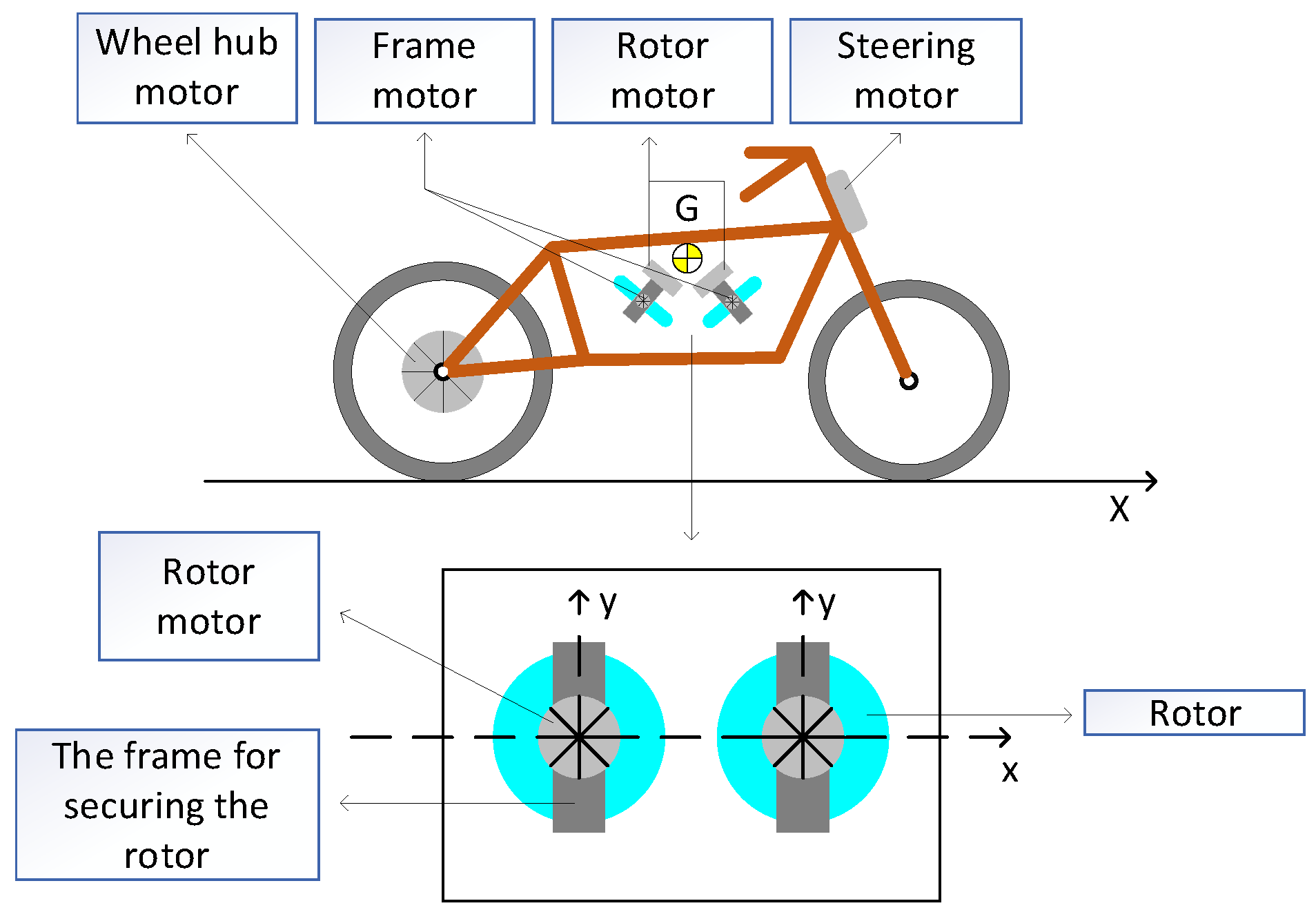
SGCMG (Single-Gimbaled Control Moment Gyroscopes) is an important space actuator, which generally consists of a rotor and a frame component. The rotor rotates at a constant angular velocity, providing a constant angular momentum. The frame assembly drives the rotor assembly to rotate around the frame axis perpendicular to the direction of the angular momentum vector, changing the direction of the angular momentum vector while outputting the gyroscopic moment. The SGCMG control used in this paper can generate large torque and has good control effect for all kinds of operating conditions of the vehicle.

According to the literature cited in this paper, it is known that the studies using the above three control methods are all validated by bikes or small prototypes. The simulation and test conditions are quite single. At the same time, the validation of the effectiveness of the control methods is quite limited, and the robustness of the controller is not systematically analyzed. In this paper, the effectiveness and robustness of the controller are fully verified based on the simulation experiments of the large mass motorcycle model with multiple working conditions and the verification of some working conditions on the real vehicle.

1.3. Contributions

This paper presents the design of a SGCMG frame angular velocity controller, it is also claimed that the controller can realize the self-balancing of linear and curvilinear motions under static and dynamic conditions of motorcycle and make the body of the motorcycle with good anti-disturbance capability. In this paper, the SGCMG frame angular velocity controller based on the feedback of the body’s angular acceleration is used for the first time to self-balance the linear and curvilinear motions of a large mass motorcycle under static and dynamic conditions, and its excellent robustness is verified by multi-case simulation experiments. Finally, the feasibility of the control algorithm was verified by porting it to a real vehicle equipped with the embedded system for testing. Section II presents the dynamics modeling of the two-wheeled motorcycle, Section III presents the design of the SGCMG frame angular velocity controller, Section IV conducts MATLAB/Simulink simulation experiments and analysis based on the dynamics model, Section V conducts the design of the Kalman filter for the actual body roll angular acceleration and the real-world testing and analysis, and finally, Section VI summarizes the above work and provides an outlook for future work.

2. System Template Background

To fully describe the overall motion of the motorcycle, six degrees of freedom are required, namely three axes of displacement, i.e., x, y, and z positions. And three axes of attitude, i.e., roll angle, pitch angle, and heading angle. This paper focuses on the equilibrium characteristics of the motorcycle, so this paper only focuses on the moment balance equations of the motorcycle in the roll direction [30].

The analytical assumptions made in this section of the modeling process are as follows:

• The contact between the front and rear wheels and the ground is point contact, and the wheel-ground friction is static (no relative sliding);
• The entire bicycle is a multi-stiff body structure (no deformation);
• The bicycle wheels are in constant contact with the ground, and the motion is considered only in the horizontal plane.

We first define the physical parameters of the vehicle used in the derivation process:

• G is the center of mass of the whole vehicle;
• $\mathsf{\alpha }$ is the precession angle of the frame;
• $\mathsf{\omega }$ is the rotational speed of the rotor, where ${\mathsf{\omega }}_1=-{\mathsf{\omega }}_2$;
• h is the height of the whole vehicle’s center of mass from the ground;
• l_r is the distance from the center of mass to the rear wheel center;
• L is the wheelbase of the vehicle, which is the distance from the front wheel center to the rear wheel center;
• r_f, r_r are the rolling radii of the front and rear wheels, respectively;
• λ is the tilt angle of the front fork;
• $\dot{\mathsf{\delta }}$ is the steering angular velocity of the handlebar;
• $\mathsf{\theta }$ is the roll angle of the car body rotating around the X-axis;
• m is the mass of the whole car;
• g is the acceleration of gravity;
• ${\mathsf{\delta }}_{\mathrm{R}}$ is the steering angle of the motion of the fork, ${\mathsf{\delta }}_{\mathrm{R}}={\tan }^{-1}(\frac{\cos (\mathsf{\lambda })\sin (\mathsf{\delta })}{\cos (\mathsf{\theta })\cos (\mathsf{\delta })-\sin (\mathsf{\theta })\sin (\mathsf{\lambda })\sin (\mathsf{\delta })})$;
• R is the radius of rotation of the whole car around the instantaneous center;
• Rf, Rr are the radii of rotation of the front and rear wheels around the instantaneous center;
• ${\mathrm{I}}_{\mathrm{o}}{, \mathrm{I}}_{\mathrm{g}}$ are the rotational inertia of the whole car around the center of mass and parallel to the rolling axis, and the rotor’s rotational inertia;
• V_f, V_r are the linear velocities of the front and rear wheels;
• a_r is the linear acceleration of the rear wheel.

Figure 1 shows the overall structure of a two-wheeled motorcycle equipped with CMG, in which various types of motors are used for the actuators. The body motion coordinate system O-XYZ and the rotor motion coordinate system o-xyz are also established.

2.1. Virtual Inertia Moment

The moment of inertia is not a real moment, but the sum of all other moments, resulting from the rotational effect of the angular acceleration, which is the rotational form of Newton’s second law.

$${\mathrm{M}=(\mathrm{I}}_{\mathrm{o}}{+\mathrm{mh}}^2){\ddot{\mathsf{\theta }}}_{\mathrm{e}}$$

(1)

2.2. Precession Moment of SGCMG

For a single moment gyro [31]:

$${\mathrm{T}}_1{=\mathrm{I}}_{\mathrm{g}}\dot{{\mathsf{\alpha }}_1}\dot{{\mathsf{\omega }}_1}{, \mathrm{T}}_2{=\mathrm{I}}_{\mathrm{g}}\dot{{\mathsf{\alpha }}_2}\dot{{\mathsf{\omega }}_2}$$

(2)

The component of the precession moment on the X and Z axes (as shown in Figure 2) of the car body:

$${\mathrm{T}}_{1\mathrm{X}}{=\mathrm{I}}_{\mathrm{g}}\dot{{\mathsf{\alpha }}_1}{\mathsf{\omega }}_1{\cos (\mathsf{\alpha }}_1), {\mathrm{T}}_{1\mathrm{Z}}{=\mathrm{I}}_{\mathrm{g}}\dot{{\mathsf{\alpha }}_1}{\mathsf{\omega }}_1{\sin (\mathsf{\alpha }}_1)$$

(3)

$${\mathrm{T}}_{2\mathrm{X}}{=\mathrm{I}}_{\mathrm{g}}\dot{{\mathsf{\alpha }}_2}{\mathsf{\omega }}_2{\cos (\mathsf{\alpha }}_2), {\mathrm{T}}_{2\mathrm{Z}}{=\mathrm{I}}_{\mathrm{g}}\dot{{\mathsf{\alpha }}_2}{\mathsf{\omega }}_2{\sin (\mathsf{\alpha }}_2)$$

(4)

In the above equation:

$$\dot{{\mathsf{\alpha }}_1}=-\dot{{\mathsf{\alpha }}_2},{\mathsf{\omega }}_1=-{\mathsf{\omega }}_2$$

Therefore:

$${\mathrm{T}}_{1\mathrm{X}}{=\mathrm{T}}_{2\mathrm{X}}{, \mathrm{T}}_{1\mathrm{Z}}=-{\mathrm{T}}_{2\mathrm{Z}}$$

So, the gyroscope produces a moment of advance ${\mathrm{T}}_{\mathrm{X}}$ around the X-axis (inverse to the Gravity moment) of:

$${\mathrm{T}}_{\mathrm{X}}{=(\mathrm{I}}_{\mathrm{g}}\dot{{\mathsf{\alpha }}_1}{\mathsf{\omega }}_1{\cos (\mathsf{\alpha }}_1{)+\mathrm{I}}_{\mathrm{g}}\dot{{\mathsf{\alpha }}_2}{\mathsf{\omega }}_2{\cos (\mathsf{\alpha }}_2{))=2\mathrm{T}}_{1\mathrm{X}}{=2\mathrm{T}}_{2\mathrm{X}}$$

(5)

2.3. Total Vehicle Weight Moment

The state of the car body when it has a roll angle is shown in the Figure 3. When the angle of the roll deviates from the vertical equilibrium point, the force arm is generated in the lateral direction of the body, and the weight moment ${\mathrm{M}}_{\mathrm{g}}$ is generated in the axial direction of the roll:

$${\mathrm{M}}_{\mathrm{g}}=\mathrm{mghsin}(\mathsf{\theta })$$

(6)

2.4. Centrifugal Moment of the Whole Vehicle Rotating around the Transient Center

2.4.1. Rear Wheel Centrifugal Acceleration a_cr

The top view of the whole vehicle rotating around the transient center is shown in Figure 4, where the rear wheel turning radius R_r around the transient center is:

$${ \mathrm{R}}_{\mathrm{r}}=\frac{\mathrm{L}}{{\tan (\mathsf{\delta }}_{\mathrm{R}})}$$

(7)

$${\mathrm{a}}_{\mathrm{cr}}=\frac{{\mathrm{v}}_{\mathrm{r}}^2}{{\mathrm{R}}_{\mathrm{r}}}=\frac{{\mathrm{v}}_{\mathrm{r}}^2{\tan (\mathsf{\delta }}_{\mathrm{R}})}{\mathrm{L}}$$

(8)

The centrifugal acceleration of the rear wheels, perpendicular to the roll axis X, forms the centrifugal moment on the roll axis, which directly affects the stability of the body.

2.4.2. Centrifugal Acceleration of the Front Wheel a_cf

The turning radius R_f of the front wheel around the transient center is:

$${\mathrm{R}}_{\mathrm{f}}=\frac{\mathrm{L}}{{\sin (\mathsf{\delta }}_{\mathrm{R}})}$$

(9)

The front wheel speed v_f is:

$${ \mathrm{v}}_{\mathrm{f}}=\frac{{\mathrm{v}}_{\mathrm{r}}}{{\cos (\mathsf{\delta }}_{\mathrm{R}})}$$

(10)

The centrifugal acceleration of the front wheel a_cf is:

$${\mathrm{a}}_{\mathrm{cf}}=\frac{{\mathrm{v}}_{\mathrm{f}}^2}{{\mathrm{R}}_{\mathrm{f}}}=\frac{{\mathrm{v}}_{\mathrm{r}}^2{\sin (\mathsf{\delta }}_{\mathrm{R}})}{{\mathrm{Lcos}(\mathsf{\delta }}_{\mathrm{R}}{)}^2}$$

(11)

The component of the centrifugal acceleration of the front wheel in the Y-axis a_cfy is:

$${\mathrm{a}}_{\mathrm{cfY}}{=\mathrm{a}}_{\mathrm{cf}}{\cos (\mathsf{\delta }}_{\mathrm{R}})=\frac{{\mathrm{v}}_{\mathrm{r}}^2{\sin (\mathsf{\delta }}_{\mathrm{R}})}{{\mathrm{Lcos}(\mathsf{\delta }}_{\mathrm{R}}{)}^2}{\cos (\mathsf{\delta }}_{\mathrm{R}})=\frac{{\mathrm{v}}_{\mathrm{r}}^2{\tan (\mathsf{\delta }}_{\mathrm{R}})}{\mathrm{L}}$$

(12)

Combining Equations (8) and (12), the centrifugal acceleration of the front wheel and the rear wheel around the instantaneous center is equal in the Y-axis, so the centrifugal acceleration along the Y-axis at the center of mass is also equal to this acceleration.

$${\mathrm{a}}_{\mathrm{ccY}}{=\mathrm{a}}_{\mathrm{cr}}{=\mathrm{a}}_{\mathrm{cfY}}=\frac{{\mathrm{v}}_{\mathrm{r}}^2{\tan (\mathsf{\delta }}_{\mathrm{R}})}{\mathrm{L}}$$

(13)

The centrifugal moment M_C of the whole vehicle around the transient center is (inverse to the heavy moment):

$${\mathrm{M}}_{\mathrm{c}}{=\mathrm{ma}}_{\mathrm{ccY}}\mathrm{hcos}(\mathsf{\theta })=\mathrm{mhcos}(\mathsf{\theta })\frac{{\mathrm{v}}_{\mathrm{r}}^2{\tan (\mathsf{\delta }}_{\mathrm{R}})}{\mathrm{L}}=\frac{1}{\mathrm{L}}{\mathrm{mv}}_{\mathrm{r}}^2\mathrm{htan}({\mathsf{\delta }}_{\mathrm{R}})\cos (\mathsf{\theta })$$

(14)

2.5. Rolling Moment from Accelerated Driving

The acceleration generated by the change of the linear velocity of the wheel will cause the acceleration of different parts of the vehicle with different magnitudes and direction, and produce the acceleration component in the Y-axis direction, which will generate the moment around the X-axis and affect the balance of the vehicle. The relevant diagram is shown below, where the point of force is the contact point between the tire and the ground, and the symbol convention is shown below.

Figure 5 shows the state of the motorcycle motion during acceleration.

The direction of the force arm points from the fulcrum to the point of force, the direction of the force arm is the fulcrum pointing to the point of force, that is, the center of mass points to the tire landing place, so the moment term in the combined moment equation in the latter part of the text needs to add a negative sign.

2.5.1. Front Wheel Line Acceleration ${\mathrm{a}}_{\mathrm{f}}$

$${\mathrm{a}}_{\mathrm{fX}}{=\mathrm{a}}_{\mathrm{r}}{=\mathrm{a}}_{\mathrm{f}}{\cos (\mathsf{\delta }}_{\mathrm{R}})$$

(15)

$${\mathrm{a}}_{\mathrm{f}}=\frac{{\mathrm{a}}_{\mathrm{r}}}{{\cos (\mathsf{\delta }}_{\mathrm{R}})}$$

(16)

The Y-Directional component ${\mathrm{a}}_{\mathrm{fy}}$ of the linear acceleration of the front wheel is:

$${\mathrm{a}}_{\mathrm{fY}}{=\mathrm{a}}_{\mathrm{f}}{\sin (\mathsf{\delta }}_{\mathrm{R}})=\frac{{\sin (\mathsf{\delta }}_{\mathrm{R}})}{{\cos (\mathsf{\delta }}_{\mathrm{R}})}{\mathrm{a}}_{\mathrm{r}}{=\tan (\mathsf{\delta }}_{\mathrm{R}}{)\mathrm{a}}_{\mathrm{r}}$$

(17)

2.5.2. The Y-Directional Component of the Acceleration at Point O

$${\mathrm{a}}_{\mathrm{OY}}=\frac{{\mathrm{l}}_{\mathrm{r}}}{\mathrm{L}}{\mathrm{a}}_{\mathrm{fy}}=\frac{{\mathrm{l}}_{\mathrm{r}}}{\mathrm{L}}{\tan (\mathsf{\delta }}_{\mathrm{R}}{)\mathrm{a}}_{\mathrm{r}}$$

(18)

2.5.3. The x-Axis Moment Generated by the Linear Acceleration of the Wheel ${\mathrm{M}}_{\mathrm{acc}}$

$${\mathrm{M}}_{\mathrm{acc}}{=\mathrm{ma}}_{\mathrm{OY}}\mathrm{hcos}(\mathsf{\theta })=\frac{{\mathrm{l}}_{\mathrm{r}}}{\mathrm{L}}{\mathrm{ma}}_{\mathrm{r}}{\mathrm{htan}(\mathsf{\delta }}_{\mathrm{R}})\cos (\mathsf{\theta })$$

(19)

2.6. Rolling Moment from Angular Velocity of Fork Steering

The angular velocity of the front fork steering axis when turning will change the direction of the front wheel’s linear velocity, resulting in acceleration. This acceleration will also have an effect on the velocity of the whole vehicle and produce an acceleration at the center of mass, thus producing an equivalent moment in the roll direction, which will have an effect on the balance of the whole vehicle. The kinetic and kinematic analysis of this factor is shown in Figure 6. The direction of the force arm is from the pivot point to the point of force. The center of mass is pointing to the tire landing point, so the moment term in the combined moment equation later in the article needs to add a negative sign.

2.6.1. Lateral Acceleration of the Center of Mass due to Fork Steering

The angular velocity of rotation $\dot{\mathsf{\delta }}$ of the front wheel velocity ${\mathrm{v}}_{\mathrm{f}}$ caused by the angular velocity ${\dot{\mathsf{\delta }}}_{\mathrm{Z}}$ of the fork steering is:

$${\dot{\mathsf{\delta }}}_{{\mathrm{Z}}^{\prime }}=\dot{\mathsf{\delta }}\cos (\mathsf{\lambda })$$

(20)

$${\dot{\mathsf{\delta }}}_{\mathrm{Z}}={\dot{\mathsf{\delta }}}_{{\mathrm{Z}}^{\prime }}\cos (\mathsf{\theta })=\dot{\mathsf{\delta }}\cos (\mathsf{\lambda })\cos (\mathsf{\theta })$$

(21)

The acceleration ${\mathrm{a}}_{\dot{\mathsf{\delta }}\mathrm{f}}$ at the front wheel junction is:

$${\mathrm{a}}_{\dot{\mathsf{\delta }}\mathrm{f}}={\dot{\mathsf{\delta }}}_{\mathrm{Z}}\times {\mathrm{v}}_{\mathrm{f}}=\dot{\mathsf{\delta }}{\mathrm{v}}_{\mathrm{f}}\cos (\mathsf{\lambda })\cos (\mathsf{\theta })$$

(22)

The lateral component ${\mathrm{a}}_{\dot{\mathsf{\delta }}\mathrm{fY}}$ of the acceleration at the front wheel junction is:

$${\mathrm{a}}_{\dot{\mathsf{\delta }}\mathrm{fY}}={\mathrm{a}}_{\dot{\mathsf{\delta }}\mathrm{f}}\cos ({\mathsf{\delta }}_{\mathrm{R}})=\dot{\mathsf{\delta }}{\mathrm{v}}_{\mathrm{f}}\cos (\mathsf{\lambda })\cos (\mathsf{\theta })\cos ({\mathsf{\delta }}_{\mathrm{R}})$$

(23)

The transverse acceleration component ${\mathrm{a}}_{\dot{\mathsf{\delta }}\mathrm{OY}}$ of the center of mass at the projection of the wheel ground line is:

$${\mathrm{a}}_{\dot{\mathsf{\delta }}\mathrm{OY}}=\frac{1_{\mathrm{r}}}{\mathrm{L}}{\mathrm{a}}_{\mathsf{\delta }\mathrm{fY}}=\frac{1_{\mathrm{r}}}{\mathrm{L}}\dot{\mathsf{\delta }}{\mathrm{v}}_{\mathrm{f}}\cos (\mathsf{\lambda })\cos (\mathsf{\theta })\cos ({\mathsf{\delta }}_{\mathrm{R}})$$

(24)

2.6.2. Rolling Moment due to Angular Velocity of Fork Steering

$${\mathrm{M}}_{{\dot{\mathsf{\delta }}}_{{\mathrm{V}}_{\mathrm{f}}}}={\mathrm{ma}}_{\dot{\mathsf{\delta }}\mathrm{OY}}\mathrm{hcos}(\mathsf{\theta })=\frac{1_{\mathrm{r}}}{\mathrm{L}}\mathrm{m}{\dot{\mathsf{\delta }}}_{{\mathrm{V}}_{\mathrm{f}}}\mathrm{hcos}(\mathsf{\lambda })\cos {(\mathsf{\theta })}^2\cos ({\mathsf{\delta }}_{\mathrm{R}})$$

(25)

The kinetic equation of the unmanned two-wheeled motorcycle equipped with SGCMG in the roll direction is obtained by the above derivation process:

$${(\mathrm{I}}_{\mathrm{o}}{+\mathrm{mh}}^2){\ddot{\mathsf{\theta }}}_{\mathrm{e}}=\mathrm{mghsin}(\mathsf{\theta })-({\mathrm{I}}_{\mathrm{g}}\dot{{\mathsf{\alpha }}_1}{\mathsf{\omega }}_1{\cos (\mathsf{\alpha }}_1{)+\mathrm{I}}_{\mathrm{g}}\dot{{\mathsf{\alpha }}_2}{\mathsf{\omega }}_2{\cos (\mathsf{\alpha }}_2))$$

$$-\frac{1}{\mathrm{L}}{\mathrm{mv}}_{\mathrm{r}}^2\mathrm{htan}({\mathsf{\delta }}_{\mathrm{R}})\cos (\mathsf{\theta })-\frac{{\mathrm{l}}_{\mathrm{r}}}{\mathrm{L}}{\mathrm{ma}}_{\mathrm{r}}\mathrm{htan}({\mathsf{\delta }}_{\mathrm{R}})\cos (\mathsf{\theta })$$

(26)

$$-\frac{{\mathrm{l}}_{\mathrm{r}}}{\mathrm{L}}\mathrm{m}\dot{\mathsf{\delta }}{\mathrm{v}}_{\mathrm{f}}\mathrm{hcos}(\mathsf{\lambda })\cos {(\mathsf{\theta })}^2\cos ({\mathsf{\delta }}_{\mathrm{R}})$$

3. Design of SGCMG Frame Angular Velocity Control

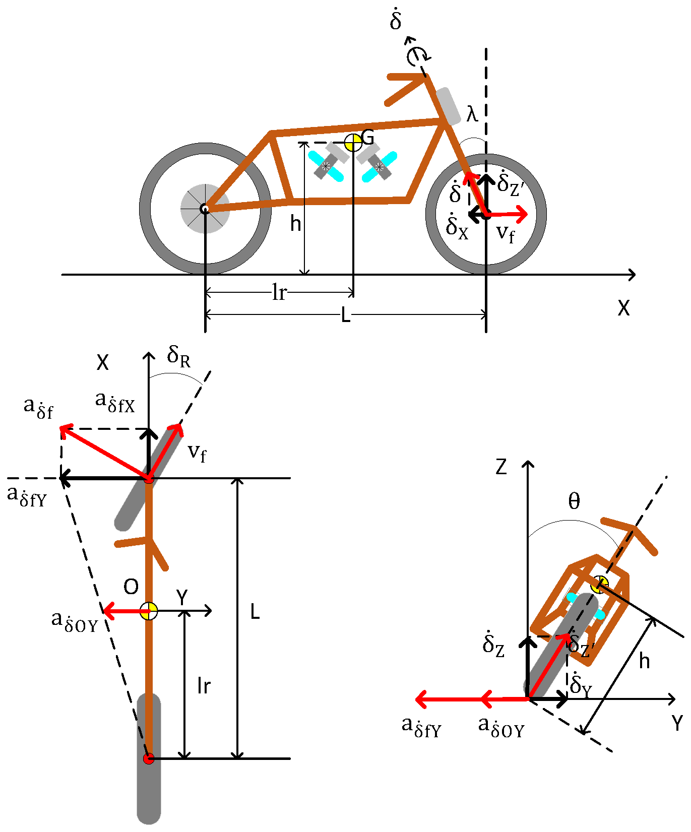
In this section, we present the design of SGCMG frame angular velocity control. The two-wheel motorcycle is a complex nonlinear system with static instability, and the relationship between the frame angular velocity $\dot{\mathsf{\alpha }}$ and the roll angular velocity $\dot{\mathsf{\theta }}$ is mainly considered after the introduction of the SGCMG model, and the roll angle $\mathsf{\theta }$, the steering angle $\mathsf{\delta }$ and the front and rear wheel linear velocities ${\mathrm{v}}_{\mathrm{f}}$ and ${\mathrm{v}}_{\mathrm{r}}$ are coupled as shown in Equation (26). In order to design the SGCMG frame angular speed controller, the nonlinear model of the two-wheeled motorcycle equipped with SGCMG needs to be simplified, and for this purpose we make the following assumptions:

• The vehicle is in a stationary non-steering state.

Based on the above assumptions, Equation (26) is linearized around $\mathsf{\theta }=0, \mathsf{\delta }=0, \mathsf{\alpha }=0$:

$${(\mathrm{I}}_{\mathrm{o}}{+\mathrm{mh}}^2)\ddot{\mathsf{\theta }}=\mathrm{mgh}\mathsf{\theta } -{ 2\mathrm{I}}_{\mathrm{g}}\dot{\mathsf{\alpha }}\mathsf{\omega }$$

(27)

Considering the motorcycle as a controlled system, the transfer function G(s) of the motorcycle is:

$$\mathrm{G}\left(\mathrm{s}\right)=\frac{\dot{\mathsf{\theta }}(\mathrm{s})}{\dot{\mathsf{\alpha }}(\mathrm{s})}=\frac{{2\mathrm{I}}_{\mathrm{g}}\mathsf{\omega }\mathrm{s}}{{(\mathrm{I}}_{\mathrm{o}}{+\mathrm{mh}}^2{)\mathrm{s}}^2- \mathrm{mgh}}$$

(28)

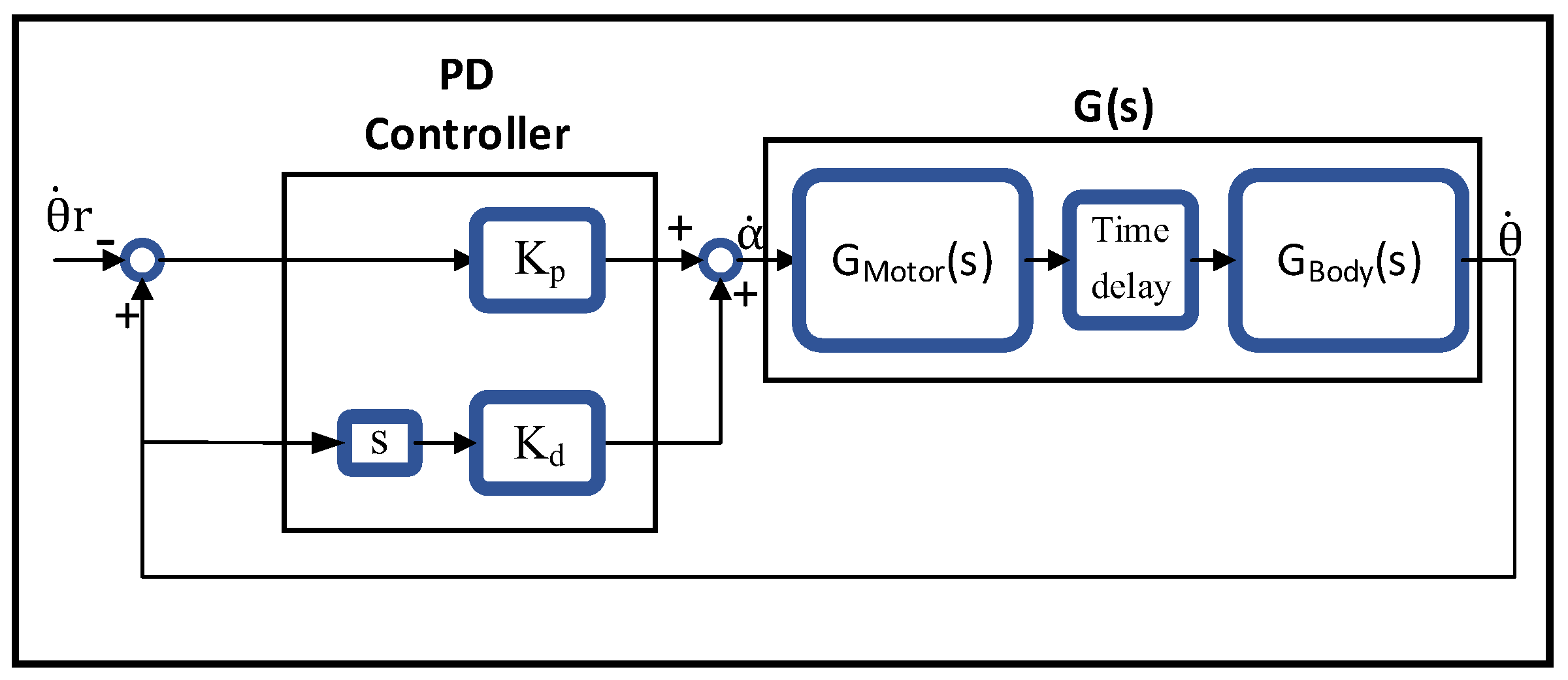
From Equation (28), we can see that only one of the two poles of the system is in the left half-plane, and the system is unstable. The condition for the equilibrium of the two-wheeled motorcycle is [$\ddot{\mathsf{\theta }}=0, \dot{\mathsf{\theta }}=0$] or [$\dot{\mathsf{\theta }}=0, \mathsf{\theta }=0$]. However, it should be noted that when the control uses [$\dot{\mathsf{\theta }},\mathsf{\theta }$] as the feedback, the car body will be balanced by sacrificing the frame angle when it is subjected to external disturbance without adding the integration link, and the singularity phenomenon exists in SGCMG, this resulting in the car body can only withstanding a rather limited continuous disturbance, and at the same time, [$\dot{\mathsf{\theta }},\mathsf{\theta }$] has a lag compared to $[\ddot{\mathsf{\theta }}]$, so the real-time control effect will also be greatly affected. Therefore, this paper chooses to design [$\ddot{\mathsf{\theta }},\dot{\mathsf{\theta }}$] as a PD controller with feedback, which will generate heavy moments to offset other moments by changing the car body’s roll angle in real time.

In the closed-loop system shown in Figure 7, the input is the desired roll angular velocity ${\dot{\mathsf{\theta }}}_{\mathrm{r}}$ and the output is the actual car body roll angular velocity $\dot{\mathsf{\theta }}$, the transfer function ${\mathrm{G}}_{\mathrm{l}}(\mathrm{s})$ of this closed-loop system is:

$${\mathrm{G}}_{\mathrm{l}}\left(\mathrm{s}\right)=\frac{\dot{\mathsf{\theta }}(\mathrm{s})}{\mathrm{R}\left(\mathrm{s}\right)}=\frac{{2\mathrm{I}}_{\mathrm{g}}{\mathsf{\omega }\mathrm{K}}_{\mathrm{p}}}{{(\mathrm{I}}_{\mathrm{o}}{+\mathrm{mh}}^2{+2\mathrm{I}}_{\mathrm{g}}{\mathsf{\omega }\mathrm{K}}_{\mathrm{d}}{)\mathrm{s}}^2{+2\mathrm{I}}_{\mathrm{g}}{\mathsf{\omega }\mathrm{K}}_{\mathrm{p}}\mathrm{s} - \mathrm{mgh}}$$

(29)

For the above closed-loop system to be stable, both poles of the transfer function ${\mathrm{G}}_{\mathrm{l}}(\mathrm{s})$ need to be in the left half-plane at the same time, ${\mathrm{s}}_1{ < 0,\mathrm{s}}_2 < 0$:

$$\mathrm{s}=\frac{-{2\mathrm{I}}_{\mathrm{g}}{\mathsf{\omega }\mathrm{K}}_{\mathrm{p}} \pm \sqrt{{{(2\mathrm{I}}_{\mathrm{g}}\mathsf{\omega })}^2{+4(\mathrm{I}}_{\mathrm{o}}{+\mathrm{mh}}^2{+2\mathrm{I}}_{\mathrm{g}}{\mathsf{\omega }\mathrm{K}}_{\mathrm{d}})(\mathrm{mgh})}}{{2(\mathrm{I}}_{\mathrm{o}}{+\mathrm{mh}}^2{+2\mathrm{I}}_{\mathrm{g}}{\mathsf{\omega }\mathrm{K}}_{\mathrm{d}})}<0$$

(30)

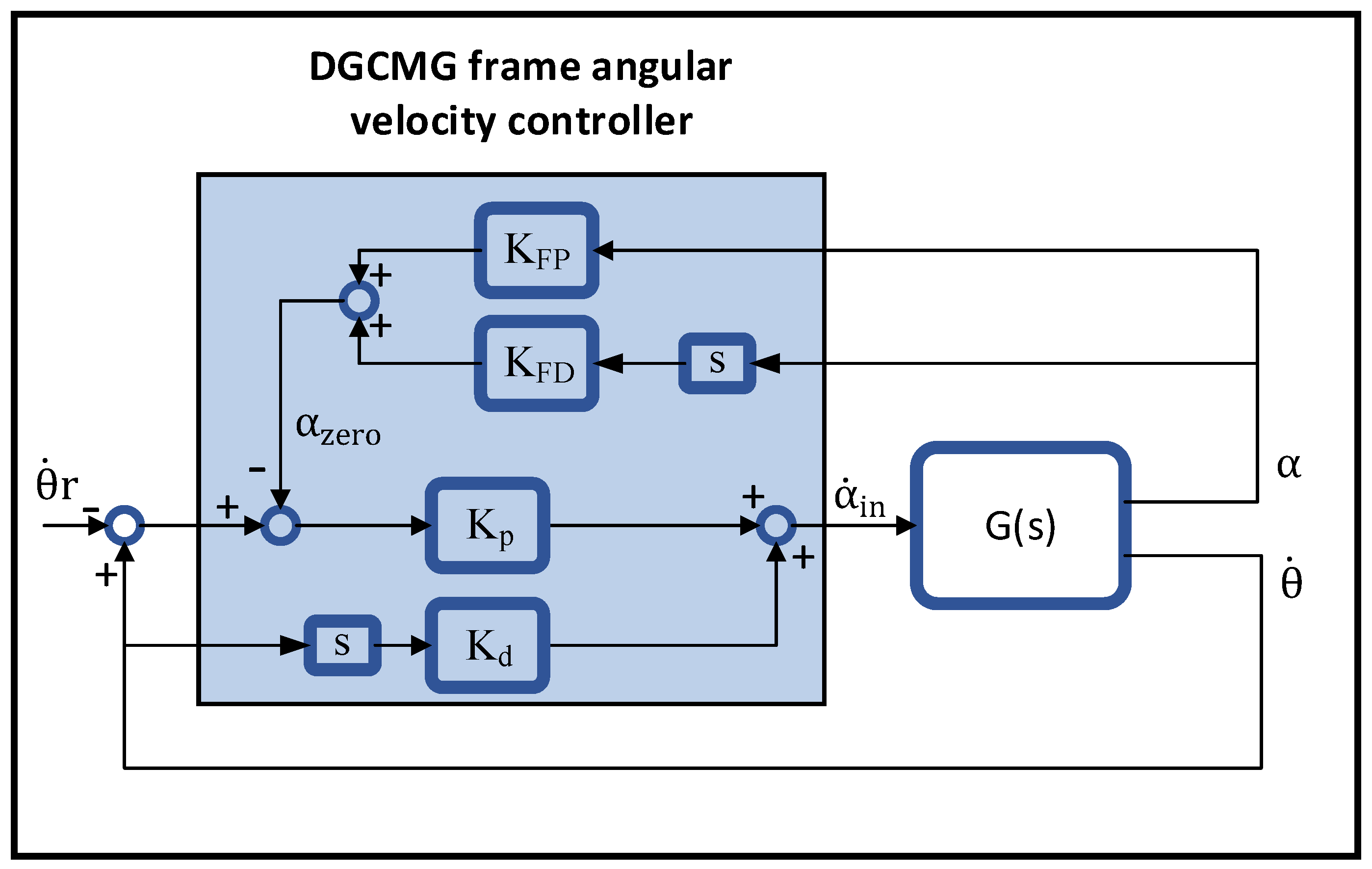
From Equation (5), it can be seen that SGCMG generates the maximum precession moment at $\mathsf{\alpha }=0$, 0 at $\mathsf{\alpha }=90°$ (singularity of SGCMG). Therefore, it is necessary to introduce a frame return to zero (frame singular avoidance) controller in the PD controller, the feedback loop equation of which is shown in Equation (31), so that the frame angle can be kept as close to 0° as possible at any time to maximize the effectiveness of the SGCMG and thus improve the impact resistance and stability of the vehicle body. The structure of the closed-loop system using the SGCMG frame angular velocity controller obtained from the above analysis is shown in Figure 8.

$${\mathsf{\alpha }}_{\mathrm{zero}}{=\mathrm{K}}_{\mathrm{FP}} ·{ \mathsf{\alpha }+\mathrm{K}}_{\mathrm{FD} }·\dot{\mathsf{\alpha }}$$

(31)

$${\dot{\mathsf{\alpha }}}_{\mathrm{in}}{=\mathrm{K}}_{\mathrm{P}}(\dot{\mathsf{\theta }}-{\dot{\mathsf{\theta }}}_{\mathrm{r}}-{\mathsf{\alpha }}_{\mathrm{zero}}{)+\mathrm{K}}_{\mathrm{d}} · \ddot{\mathsf{\theta }}$$

(32)

4. Simulation of Controller

This section shows that the SGCMG frame angular velocity controller can stabilize the motorcycle and has good robustness in the simulation. The parameters of the motorcycle prototype were obtained heuristically by measuring and estimating, as shown in

Table 1. Parameters of motorcycle and SGCMG.

Parameters	Value	Unit
m	256	kg
g	9.8	m/s2
h	0.46	m
lr	0.625	m
L	1.6	m
λ	0.5114	rad
rr	0.29	m
rf	0.28	m
ω	314.1593	rad/s
Ig	0.2	kg $·$ m2
IO	89.1696	kg $·$ m2

. According to Equation (30), it is known that ${\mathrm{K}}_{\mathrm{p}}{ > 34, \mathrm{K}}_{\mathrm{d}} > 0.7$.

Simulation experiments were conducted using MATLAB/Simulink on a Windows platform equipped with an Intel i7-10700 processor, where the simulation environment of Simulink is shown in Figure 9, and the above simulation uses the ode4 solver with a step size of 0.01. The noise in the actual system is not considered in this section, but the rotor speed and frame angular velocity are limited to ${\dot{\mathsf{\alpha }}}_{\max }$ = 2 pi rad/s, ω = 314.1593 rad/s in consideration of the actual efficiency of SGCMG and the following effect of the motor. In addition, considering the delay in the actual system and the command following speed of the motor, we try to restore the actual system in this section by introducing the time delay T₁ = 0.015 s and the transfer function ${\mathrm{G}}_{\mathrm{Motor}}{(\mathrm{s})=\mathrm{20,000}/(\mathrm{s}}^2+170\mathrm{s}+\mathrm{20,000})$ of the actual frame motor are introduced in the output frame angular velocity link shown in Figure 7 to improve the realism of the simulation.

The actual frame motor system consists of a DC servo motor, driver, and reducer. Among them, the motor is controlled by a matching drive with its own internal PID algorithm for motor speed control. The specific parameters of the motor system are given in

Table 2. DC servo motor parameter table.

Motor Model	Power (W)	Rated Voltage (VDC)	Rated Torque (N•M)	Rated Rotation Speed (rpm)	Rated Current (A)
DMKE 60TM-01330C5-C	400	48	1.27	3000	11 $\pm$ 10%

,

Table 3. Parameter table of matching drive.

Drive Model	Supply Voltage (VDC)	Switching Frequency (kHz)	Rated Current (A)	Peak Current (A)
ONKE DCPC-09016-E	20–90	15	16	48

and

Table 4. Parameter table of matching reducer.

Reducer Type	Size (mm)	Reduction Ratio
NMRV	30	1:50

.

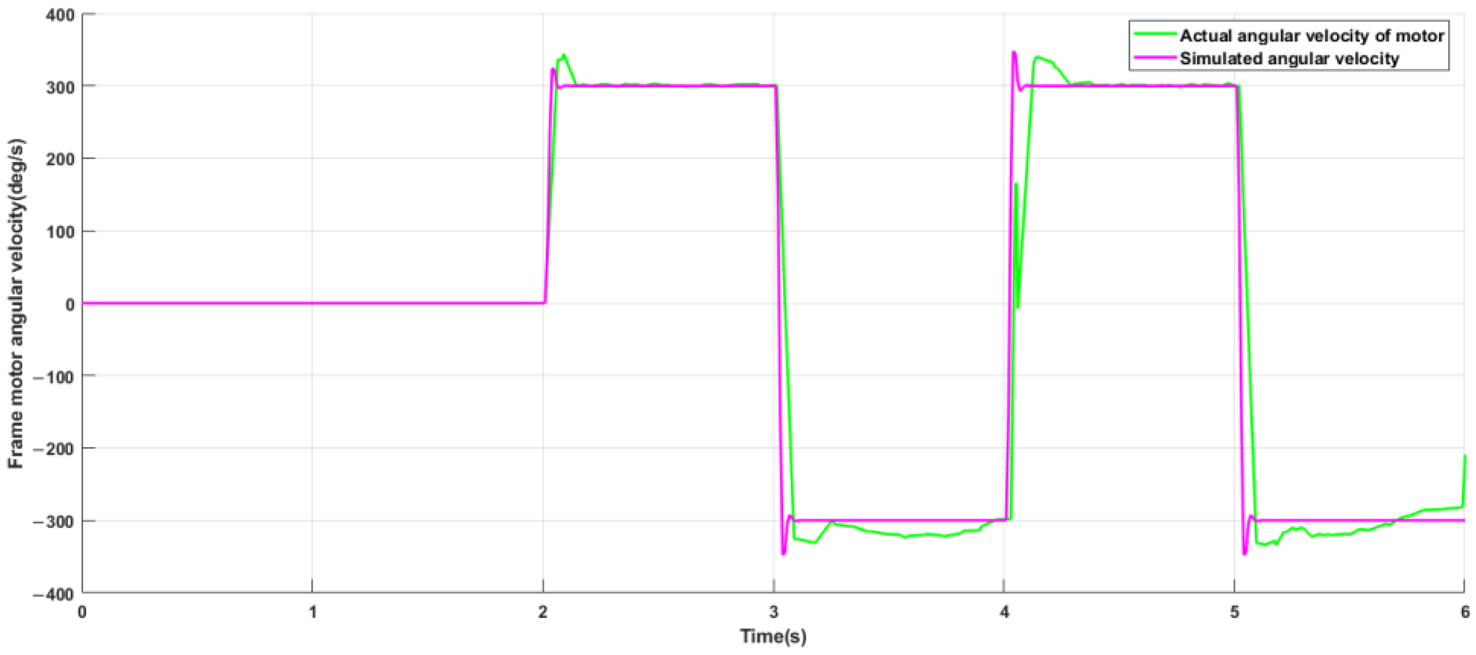
As can be seen from Figure 10, the output curve of the transfer function with the introduction of the time delay is a good fit to the output curve of the actual motor.

The control parameters are shown in

Table 5. Control parameters of the simulation.

Parameters	Value
Kp	35
Kd	6.15
KFP	−0.2
KFD	−0.265

. It is important to note that the robustness [32] of the control algorithm has a great impact on the control effect, so the robustness of the SGCMG frame angular velocity controller to changes in the parameters of the vehicle model and changes in the motion state of the vehicle needs to be analyzed next.

4.1. Robustness Analysis of Model Parameter Changes

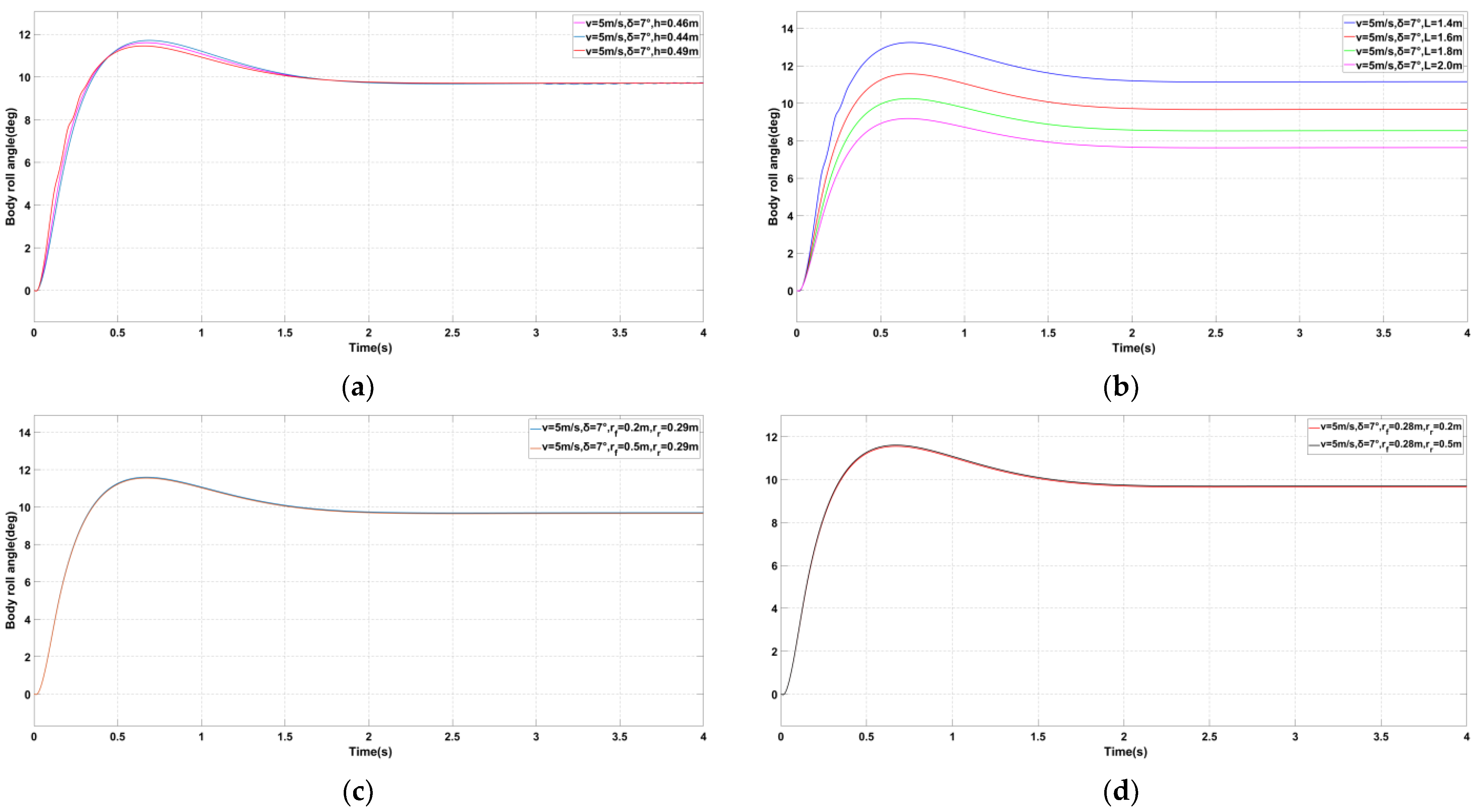
According to Equation (26), the self-balancing effect of the two-wheeled motorcycle body is related to parameters such as the wheelbase, tire size, center of mass height, and body mass. However, not all parameters will significantly affect the control effect. Therefore, the weight analysis of the parameters affecting the control effect needs to be carried out. The specific analysis process is shown in Figure 11.

Since the body model in this paper is based on the rigid body model of an unmanned motorcycle and the overall structure of the motorcycle does not undergo significant deformation during actual operation, small changes in parameters such as the body size and the height of the center of mass have little effect on the control effect of the controller. However, when the motorcycle is carrying people or goods, the mass of the motorcycle will change significantly. From Equation (26), it can be seen that the overall vehicle mass can significantly affect the overall vehicle stability. Therefore, it is necessary to carry out the robustness analysis of the controller for the variation of the vehicle mass.

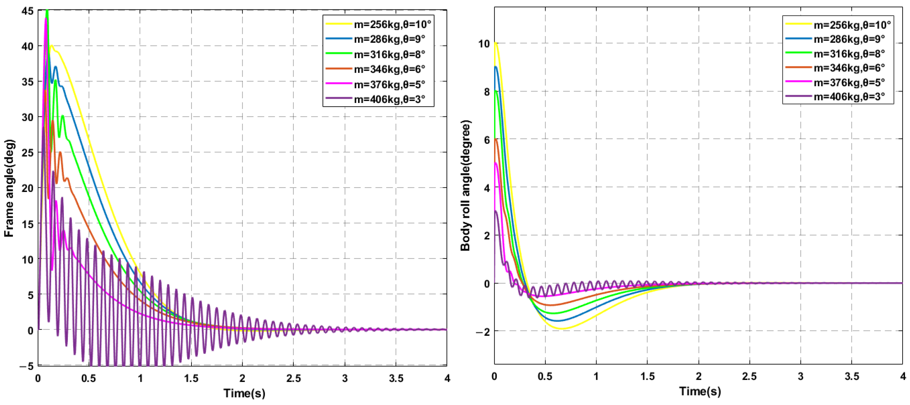
The minimum load mass of a normal motorcycle is 150 kg, so the robustness of the controller for the variation of the whole vehicle mass is analyzed in the range of 256–406 kg.

The fluctuations of the state [$\mathsf{\alpha }, \mathsf{\theta }$] with time for the case of the vehicle body at rest without steering angle and with an initial roll angle “θ” and changing the vehicle mass m are given in the Figure 12. From the above figure, it can be seen that changing the vehicle mass without changing the control parameters has a small effect on the control effect of the controller, where m = 406 kg (150 kg body load) is too large and the limited precession moment output by SGCMG weakens the control effect of the controller, resulting in a more violent vehicle shaking. At the same time, the limited feeding torque will make the maximum swing angle of the vehicle decrease with the increase of the vehicle mass.

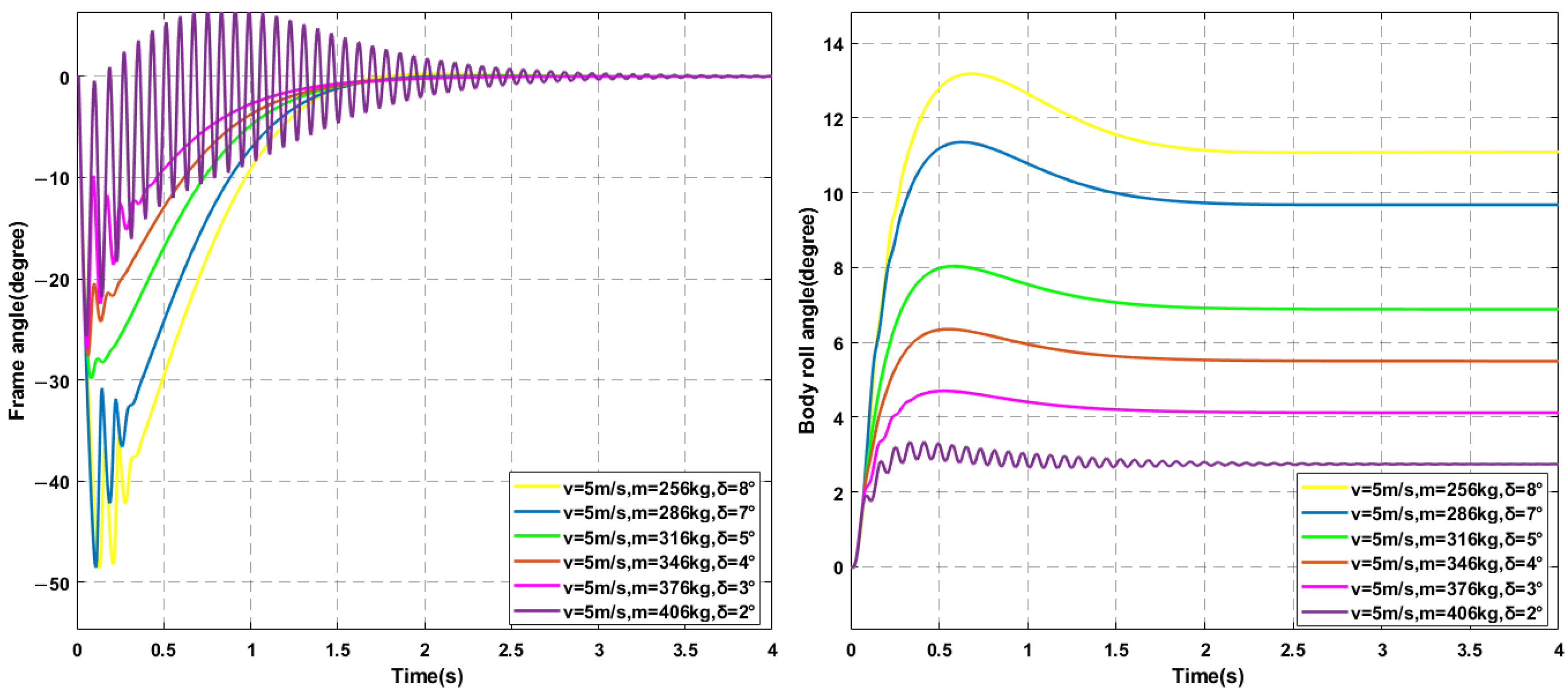
The fluctuations of the state [$\mathsf{\alpha }, \mathsf{\theta }$] with time for a vehicle speed of 5 m/s, having an initial steering angle δ and changing the whole vehicle mass m are given in Figure 13. In summary, the SGCMG frame angular velocity controller designed in this paper has good robustness to the whole vehicle mass change.

4.2. Robustness Analysis of Model Motion State Changes

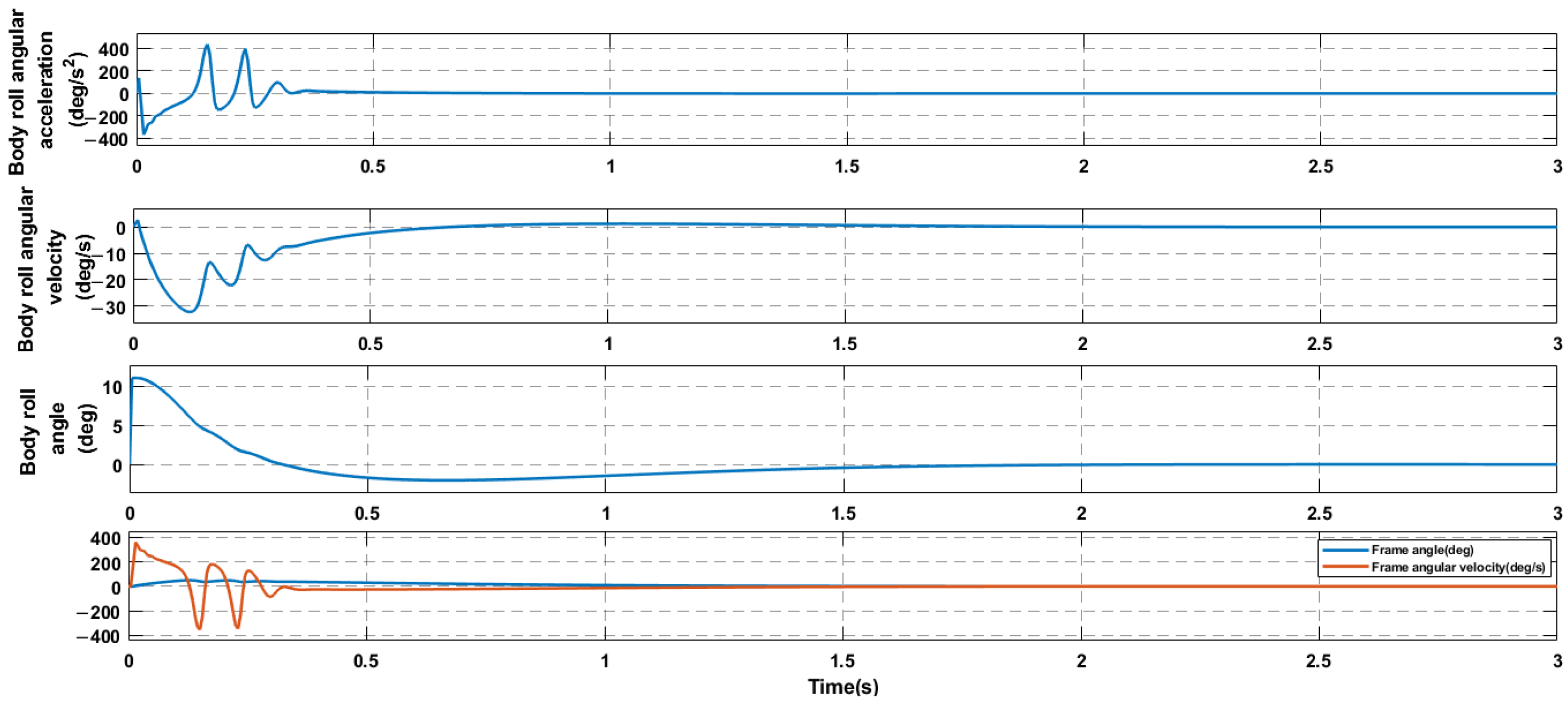
The states [$\ddot{\mathsf{\theta }},\dot{\mathsf{\theta }}$, θ, α] and the fluctuations of the system output $\dot{\mathsf{\alpha }}$ with time are given in Figure 14 for the case of a stationary vehicle with no steering angle and an initial traverse angle ${\mathsf{\theta }}_0$. From Figure 14, the initial states are [127.7°/s², 2.6°/s, 11°, 0°] and the target roll angular velocity ${\dot{\mathsf{\theta }}}_{\mathrm{r}}$ = 0°/s. The simulation results show that the state converges quickly to [0°/s², 0°/s, 0°, 0°] in 1.9 s.

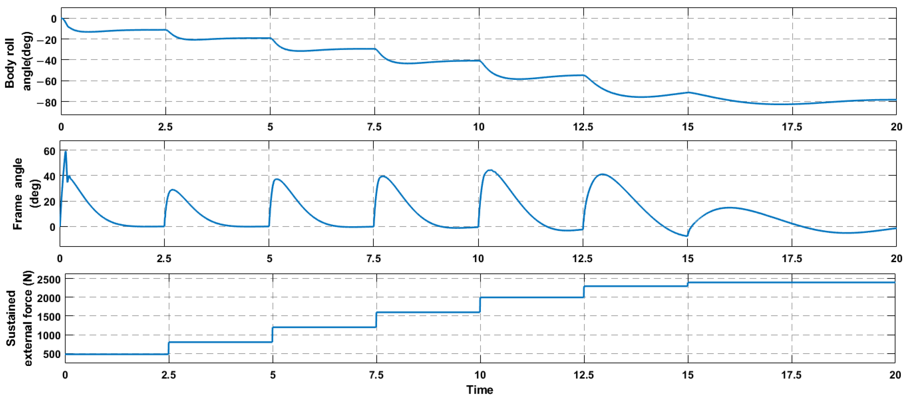
The states [$\mathsf{\theta }, \mathsf{\alpha }$] and the fluctuations of the applied external force perpendicular to the OXZ plane at the center of mass with time for the case of the car body at rest without steering and without the initial roll angle are given in Figure 15. From Figure 15, it can be seen that with the change of applied external force, the car body roll angle converges to a new equilibrium point under the control of the SGCMG frame angular velocity controller, and the roll angle that keeps the car body stable reaches −80° when the applied external force is 2400 N, which shows that the SGCMG frame angular velocity controller has a good ability to withstand the continuous disturbance. However, it should be noted that the external force application process in Figure 14 is relatively slow because the moment generated by SGCMG is limited by the frame angular velocity and rotor speed, so the car body cannot directly withstand a large, continuous external disturbance. The maximum sustained external force that can be directly applied to the car body under the condition of ${\dot{\mathsf{\alpha }}}_{\max }$ = 2 pi rad/s, ω = 314.1593 rad/s is 475 N.

The fluctuation of the instantaneous impact applied at the center of mass perpendicular to the OXZ plane with time is given in Figure 16 for the state [$\mathsf{\theta }, \mathsf{\alpha }$] of the vehicle body at rest without steering and without an initial roll angle. Considering that the collision time in the actual working condition should be much less than 0.04 s, the instantaneous impact at the center of mass of the actual car body should be much larger than 2850 N, which shows that the angular velocity controller of SGCMG frame has good resistance to transient the instantaneous shocks.

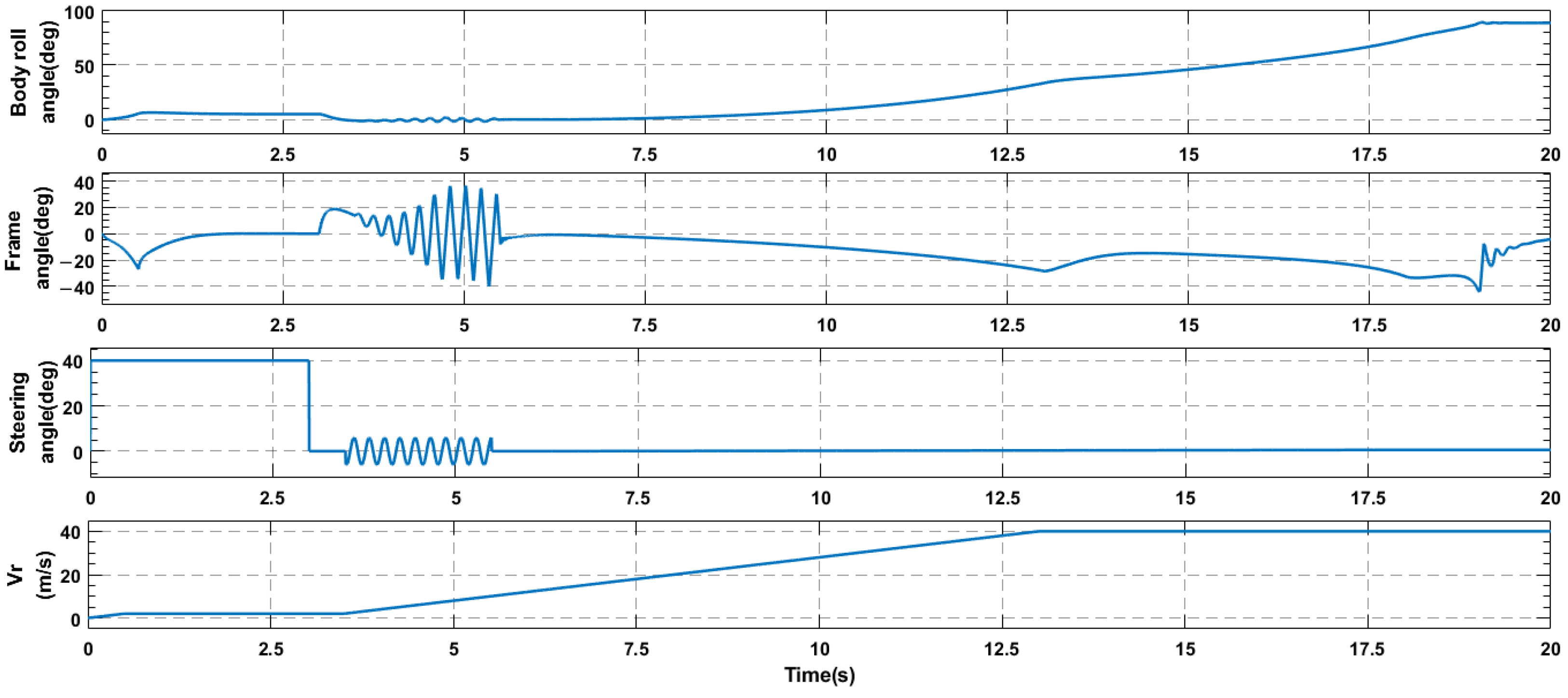
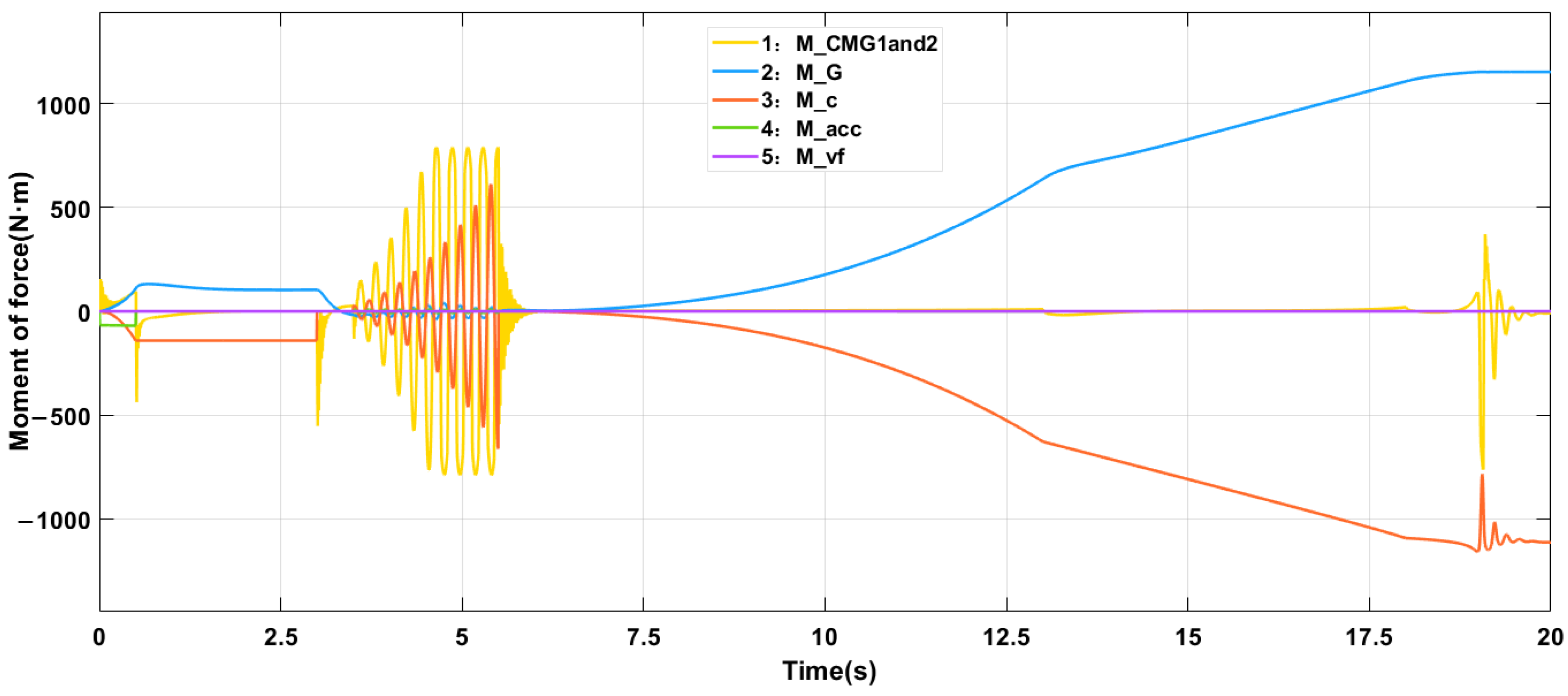
The states [${\mathsf{\theta }, \mathsf{\delta }, \mathrm{v}}_{\mathrm{r}}, \mathsf{\alpha }$] and the current fluctuations of various moments generated by the vehicle body with time are shown in Figure 17 and Figure 18, respectively, under dynamic driving conditions. It can be found that the angular velocity of the SGCMG frame can control the car body to complete the curve motion of 40° steering at low speed, the S steering motion with 6° steering amplitude and 15 rad/s frequency during acceleration, and the extreme bending motion of 0.6° steering at 40 m/s with an 88° roll angle. It can be seen that the controller has good dynamic adjustment ability for the vehicle self-balance.

From Figure 19 and

Table 6. Gain set of steering control parameters.

V(m/s)	K1	K2
1.5	4.5	11
2.0	3.0	8.0
3.0	2.0	5.0
4.0	1.75	3.5
5.0	1.0	1.75

, it can be seen that the steering controller designed in real vehicle test has extremely poor robustness for wheel speed variation, and a smaller wheel speed variation requires a significant change in the control parameters to ensure the control effect of the controller. In contrast, it can be seen from Figure 17 that the SGCMG frame angular velocity controller designed in this paper can control the vehicle at a stable speed of 0–40 m/s without changing the control parameters, which fully proves that the controller in this paper has good robustness and stability for wheel speed variation.

The above simulation results show that the SGCMG frame angular velocity controller is similar to the control of the instantaneous mass distribution of the “human-vehicle” system when a person rides a bicycle. For example, a racer in a small corner press at high speed mainly uses his body hanging to the side of the car body to make the system weight moment greater than the centrifugal moment to achieve the required roll angle for cornering. The human uses his own gravity to make the “human-vehicle” system move to the target balance state. The SGCMG frame angular velocity controller proposed in this paper replaces the weight moment applied to the vehicle body by generating the precession moment to control the movement of the vehicle body to the required roll angle for balance, which is in accordance with the motorcycle dynamics. The above simulation results also fully demonstrate the good robustness of the SGCMG frame angular velocity controller under various operating conditions for wheel speed variation, steering angle variation, acceleration variation, and external disturbance. However, it should be noted that the control effect of the controller depends on the performance of the SGCMG. As the precession moment generated by the SGCMG increases (frame angular velocity increases, rotor speed increases), the attitude change response, anti-interference ability, dynamic adjustment ability, and load capacity of the vehicle will be substantially improved.

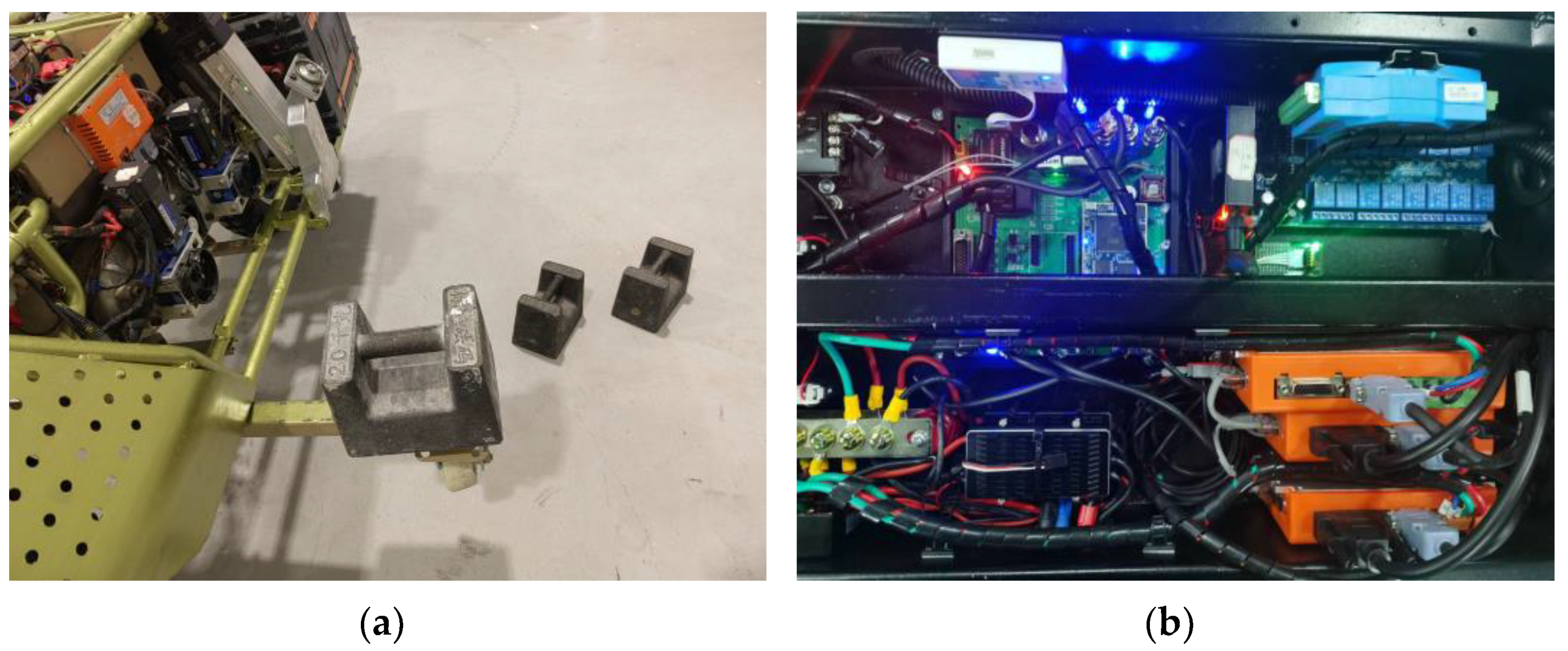
5. Experiments on Prototype

In order to verify the effectiveness of the SGCMG frame angular velocity controller, an experimental prototype, as shown in Figure 20a, was constructed for static tests (The complete physical picture of the prototype cannot be uploaded due to the confidentiality of the project). The prototype controller is an embedded system with a STM32H743 core board, as shown in Figure 20b, and all of its code was co-written by the authors of this paper using third-party software, Keil V5, instead of using model-based software to generate the code. The information of above core board and Keil V5 are given in the

Table 7. Information of the STM32H743.

Core Boar Model	Chip Model	Main Frequency (MHz)	FLASH Capacity (B)	SRAM Capacity (B)
STM32H743	STM32H743IIT6	480	2048 K	1060 K

and

Table 8. Information of the Keil V5.

Software Name	Supported Devices	Compiler Language	Software Tools
Keil V5	Cortex-M/Cortex-R4	C	Editor
	ARM7/ARM9	C++	Compiler

. Furthermore, the parameters of the prototype are different from the simulated parameters in several places, and the relevant parameters are given in

Table 9. Parameters of the prototype.

Parameters	Value	Unit
mr	320	kg
g	9.8	m/s2
hr	0.52	m
λr	0	rad
ωr	314.1593	rad/s

.

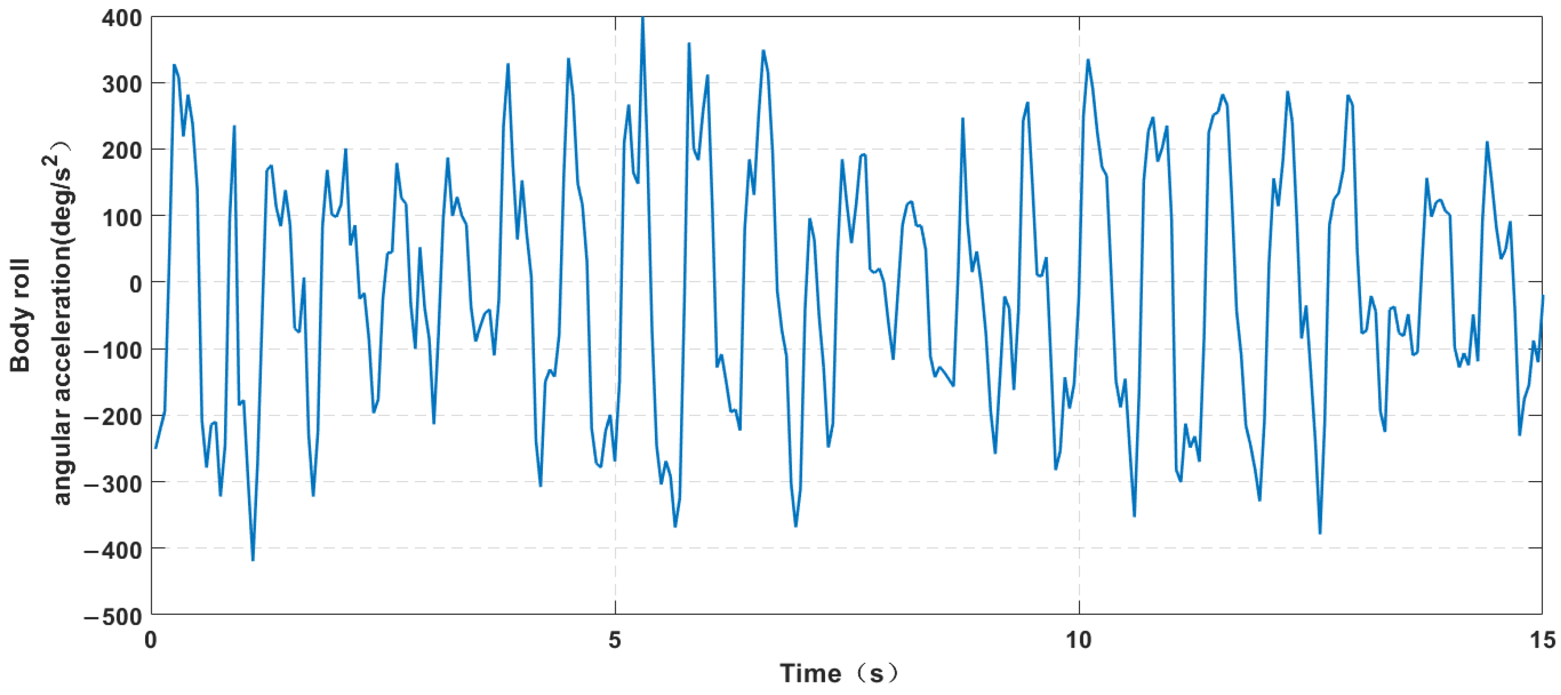
The quality of the feedback signal collected by the IMU needs to be evaluated before conducting the controller validation test. Since [$\dot{\mathsf{\theta }},\mathsf{\theta },\mathsf{\alpha },\dot{\mathsf{\alpha }}$] can all be captured directly by the IMU and frame motor driver, but the $\ddot{\mathsf{\theta }}$ signal cannot be output directly through the IMU, so the $\dot{\mathsf{\theta }}$ output from the IMU in the case of stationary running SGCMG is evaluated by unfolding the data after three-point differencing, and the ${\ddot{\mathsf{\theta }}}_{\mathrm{diff}}$ is obtained, as shown in Figure 21.

From Figure 21, it can be seen that the ${\ddot{\mathsf{\theta }}}_{\mathrm{diff}}$ signal is of very poor quality in the case of stationary running SGCMG, and the amplitude and frequency of the signal are too high for the controller to use it as a feedback signal. Therefore, this chapter considers the filtering of the $\ddot{\mathsf{\theta }}$ signal. Since the controller designed in this paper needs to control the $\ddot{\mathsf{\theta }}$ of the car body, the real-time requirement of the $\ddot{\mathsf{\theta }}$ signal is strict, so the Kalman filtering method is used to process the ${\ddot{\mathsf{\theta }}}_{\mathrm{diff}}$ signal in this section.

Kalman filtering is an algorithm that uses the state equation of a linear system to optimally estimate the system state from the input and output observations of the system. Since the observed data includes the influence of noise and disturbances in the system, the optimal estimation can also be regarded as a filtering process.

The Kalman filter contains five equations: a set of time update equations (two for prediction) and a set of measurement update equations (three for correction). The time update equations are executed at each moment k of the filter operation. In the prediction phase, the Kalman filter uses the state estimate of the previous moment k − 1 to make a state estimate of the current moment k. In the update phase, the filter uses the state observations for moment k to optimize the predicted values obtained in the prediction phase for moment k to obtain a more accurate new estimate for moment k.

Prediction (set of two time-update equations):

$${\hat{\mathrm{x}}}_{\mathrm{k}}^{-}{=\mathrm{A}\hat{\mathrm{x}}}_{\mathrm{k}-1}{+\mathrm{Bu}}_{\mathrm{k}}$$

(33)

$${\mathrm{P}}_{\mathrm{k}}^{-}{=\mathrm{AP}}_{\mathrm{k}-1}{\mathrm{A}}^{\mathrm{T}}+\mathrm{Q}$$

(34)

where ${\hat{\mathrm{x}}}_{\mathrm{k}}^{-}$ is the state pre-estimate at moment k, A,B are the state transfer matrices, ${\hat{\mathrm{x}}}_{\mathrm{k}-1}$ is the state estimate at moment k − 1, ${\mathrm{u}}_{\mathrm{k}}$ is the system input at moment k (in the case of the text, there is no such item), ${\mathrm{P}}_{\mathrm{k}}^{-}$ is the pre-estimate error covariance (a measure of the error between the state estimate and the true value) at moment k, ${\mathrm{P}}_{\mathrm{k}-1}$ is the estimate error covariance at moment k − 1, and Q is the covariance matrix of the predicted values.

Update (set of three measurement update equations):

$${\mathrm{K}}_{\mathrm{k}}{=\mathrm{P}}_{\mathrm{k}}^{-}{\mathrm{H}}^{\mathrm{T}}{/(\mathrm{HP}}_{\mathrm{k}}^{-}{\mathrm{H}}^{\mathrm{T}}+\mathrm{R})$$

(35)

$${\hat{\mathrm{x}}}_{\mathrm{k}}{=\hat{\mathrm{x}}}_{\mathrm{k}}^{-}{+\mathrm{K}}_{\mathrm{k}}{(\mathrm{z}}_{\mathrm{k}}-{\mathrm{H}\hat{\mathrm{x}}}_{\mathrm{k}}^{-})$$

(36)

$${\mathrm{P}}_{\mathrm{k}}=(\mathrm{I}-{\mathrm{K}}_{\mathrm{k}}{\mathrm{H}) \mathrm{P}}_{\mathrm{k}}^{-}$$

(37)

where ${\mathrm{K}}_{\mathrm{k}}$ is the Kalman gain at moment k, ${\hat{\mathrm{x}}}_{\mathrm{k}}$ is the state estimate at moment k, ${\mathrm{P}}_{\mathrm{k}}$ is the estimation error covariance at moment k, ${\mathrm{z}}_{\mathrm{k}}$ is the measurement at moment k, H is the state transfer matrix, I is the unit matrix, and R is the covariance matrix of the measurement.

Combining the above kinetic model as a prediction and ${\ddot{\mathsf{\theta }}}_{\mathrm{diff}}$ as an observation, given the above equation: A = H = I = 1, Q = 0.1, R = 10, ${\mathrm{P}}_0=1, {\mathrm{P}}_0^{-}=0.005$, ${\hat{\mathrm{x}}}_{\mathrm{k}-1}={\ddot{\mathsf{\theta }}}_{\mathrm{e}}$, ${\mathrm{z}}_{\mathrm{k}}={\ddot{ \mathsf{\theta }}}_{\mathrm{diff}}$, the following equation is obtained:

$${\hat{\mathrm{x}}}_{\mathrm{k}}^{-}={\ddot{\mathsf{\theta }}}_{\mathrm{e}}$$

$${\mathrm{P}}_{\mathrm{k}}^{-}{=\mathrm{P}}_{\mathrm{k}-1}+\mathrm{Q}$$

$${\mathrm{K}}_{\mathrm{k}}{=\mathrm{P}}_{\mathrm{k}}^{-}{/(\mathrm{P}}_{\mathrm{k}}^{-}+\mathrm{R})$$

$${\hat{\mathrm{x}}}_{\mathrm{k}}{=\hat{\mathrm{x}}}_{\mathrm{k}}^{-}{+\mathrm{K}}_{\mathrm{k}}({\ddot{\mathsf{\theta }}}_{\mathrm{diff}}-{\hat{\mathrm{x}}}_{\mathrm{k}}^{-})$$

$${\mathrm{P}}_{\mathrm{k}}=(1-{\mathrm{K}}_{\mathrm{k}}{) \mathrm{P}}_{\mathrm{k}}^{-}$$

After using the above Kalman filter, the ${\ddot{\mathsf{\theta }}}_{\mathrm{KF}}$ is shown in Figure 22.

As can be seen from the above figure, the quality of the ${\ddot{\mathsf{\theta }}}_{\mathrm{KF}}$ signal after Kalman filtering is greatly optimized compared to ${\ddot{\mathsf{\theta }}}_{\mathrm{diff}}$, but there is a static difference in ${\ddot{\mathsf{\theta }}}_{\mathrm{KF}}$, which is caused by the angular error in the Gravity moment part of the a priori estimate in Kalman filtering, which is determined by the current roll angle of the vehicle and the balance angle of the vehicle itself. In the practical application of the controller, this static difference is offset by the frame angle.

Before starting the control verification, it should be noted that the two frames of the SGCMG may not be synchronized during the actual motion, so it is necessary to synchronize the two frame angles, i.e., to introduce the following frame synchronization loop:

$${\dot{\mathsf{\alpha }}}_{\mathrm{syn}}{=\mathrm{K}}_{\mathrm{syn}}{(\mathsf{\alpha }}_1-{\mathsf{\alpha }}_2)$$

(38)

$${\dot{\mathsf{\alpha }}}_{\mathrm{ctrl}}={\dot{ \mathsf{\alpha }}}_{\mathrm{syn}}{+\dot{\mathsf{\alpha }}}_{\mathrm{in}}$$

(39)

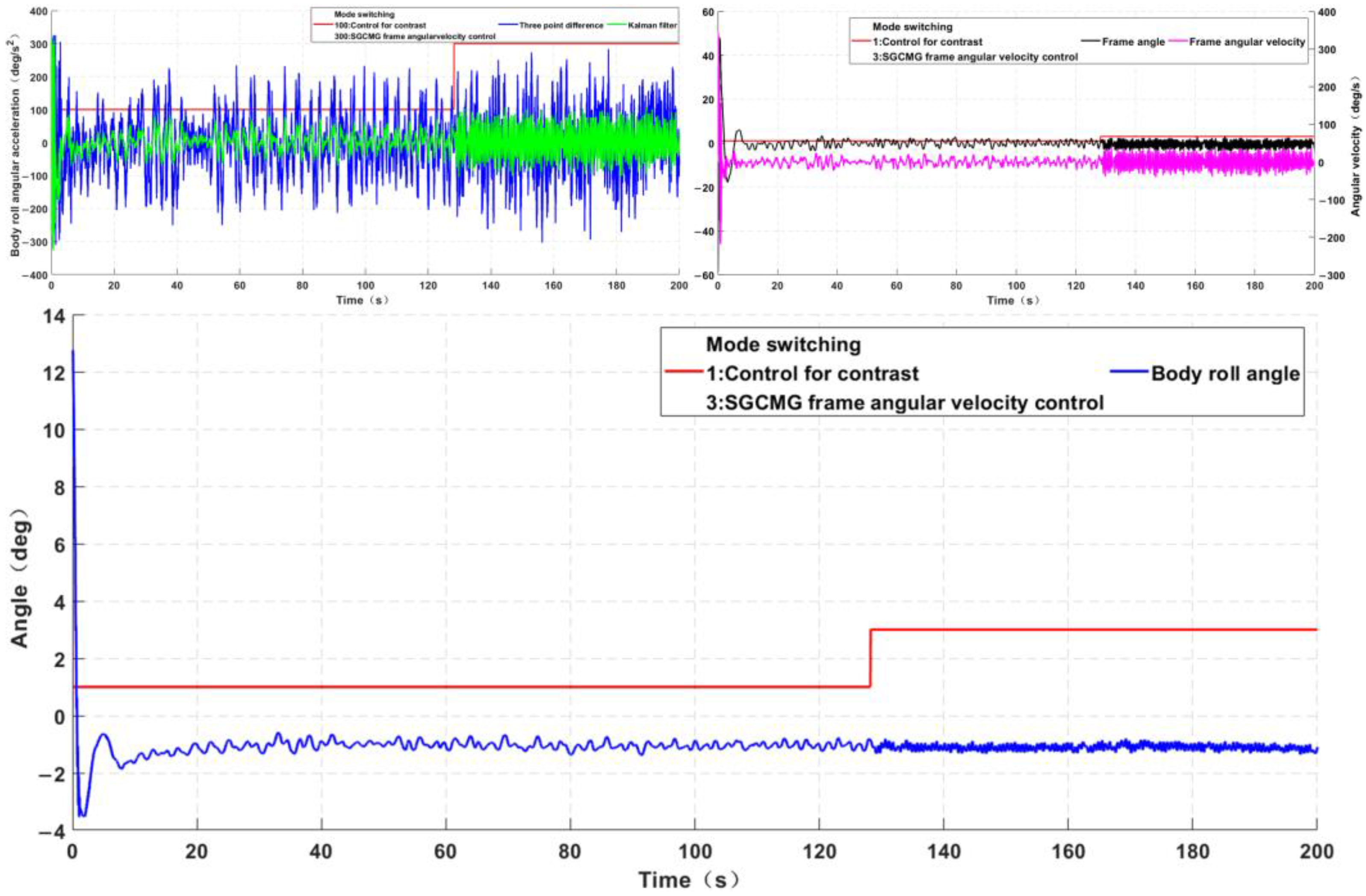
Before the verification test, it should be noted that the prototype is equipped with a protective wheel structure to ensure the safety of the vehicle, so the initial roll angle ${\mathsf{\theta }}_0 \approx \pm 13°$ (the roll angle is positive to the left from the rear-view direction) and the initial balance roll angle ${\mathsf{\theta }}_{\mathrm{B}} \approx -1°$ under the stationary state. In order to better prove the performance of the above controllers, this chapter introduces the controller based on $\dot{\mathsf{\theta }}$, θ feedback as a contrast control experiment to improve the credibility of this paper. The self-balancing process with the two controllers when the prototype is stationary, without steering angle and load, is shown in Figure 23.

From the above figure, it can be seen that the $\mathsf{\theta }$ of the car body changes more frequently and the $\ddot{\mathsf{\theta }}$ amplitude of the car body is larger after switching the controller, which is due to the adoption of the roll angular acceleration feedback to improve the real time performance of the SGCMG frame angular velocity controller, resulting in a more dramatic control effect. Meanwhile, it can be found from the figure that the balance angle of the car body before and after the controller switching does not change, both are about −1°, and the SGCMG frame angular velocity controller does not define any parameters about the target roll angle, which is consistent with the simulation results, fully proving that the controller can control the car body to find the current balance angle in real time in practical applications. In addition, the above figure shows that there is no static difference between ${\ddot{\mathsf{\theta }}}_{\mathrm{KF}}$ when the car body is moving around the equilibrium angle, which verifies the explanation of ${\ddot{\mathsf{\theta }}}_{\mathrm{KF}}$ static difference in the above paper.

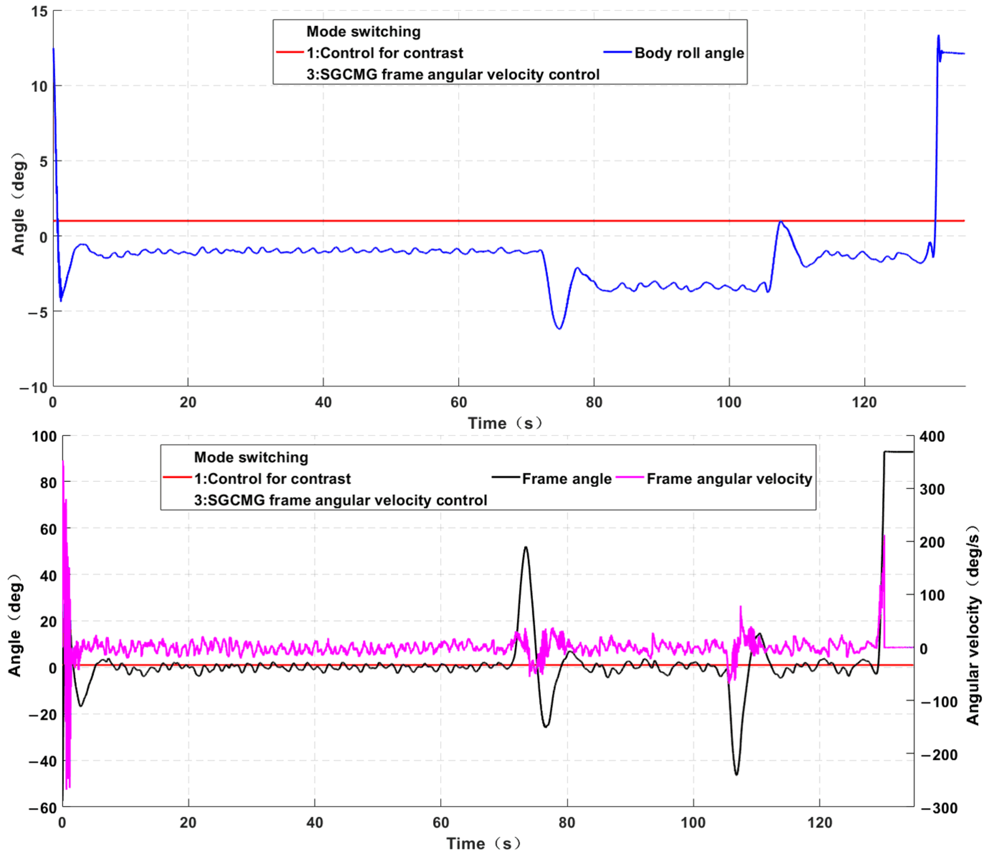
The details of the prototype load test are shown in Figure 20a, and it should be noted that the effect of the external force on the balance of the vehicle is directly related to the length of the force arm. The force arm of this test is 0.6 m, which is a more extreme test condition. The specific procedure of the test is as follows: after using the above two controllers to make the car body self-balance, place a 10 kg weight at the left side of the protective wheel in the rear view of the car, then observe the balancing state of the car body, remove the weights quickly after the car body is stable, and observe the stable state of the car body at the same time, and finally, 20 kg of weights are placed at the protective wheel quickly and observe the self-balancing process of the car body. The data obtained from the test are shown in Figure 24 and Figure 25.

The 10 kg weights are placed at the 70 s, the weights are removed at the 106.5 s, and the 20 kg weights are placed at the 129 s. From the above figure, it can be seen that when the 10 kg weight is placed for the first time, the equilibrium angle of the car is about −3.2°, the convergence time is about 10.6 s, and the overshoot is −3°. The load mass corresponding to the change of gravity at this time is about 12 kg, which is consistent with the actual working condition. The feedback signal $\dot{\mathsf{\theta }}$, θ required by the controller at the moment of load application has a hysteresis, at this time, the controller has no output, the car body will rotate a certain angle under the action of external force until the precession moment generated by SGCMG is greater than the sum of the current external moment and the weight moment, then the car body will reverse the rotation to find the current balance angle, during this period, the frame will keep turning in the positive direction until the car body passes the current balance angle ($\mathsf{\theta }=-3.63°,\dot{\mathsf{\alpha }}=-4.8°/\mathrm{s}, \mathsf{\alpha }=51.94°$ at 73.36 s), when the controller outputs the reverse frame angular velocity to control the car body to converge to the equilibrium angle gradually. However, due to the small placement weight, the smaller the angle and angular velocity of the car body rotating in the direction of the external force, the smaller the applied continuous external force, the smaller the frame angle required to find the current car body target equilibrium angle, and the faster the response of the controller to control the car body to reach steady state. In addition, it should be noted that the frame of the controller based on $\dot{\mathsf{\theta }}$, θ feedback is theoretically unable to return to zero when the body is subjected to a continuous external force, and the controller needs to offset the current angle error by the output of the frame return loop. In the above figure, the frame can return to zero due to the addition of an integral link in the zero-return loop, at the expense of some dynamic performance.

The 20 kg weight was placed at 129 s, the car body was out of balance directly after two rotations, and the frame was rotated to the limiting angle, as can be seen from the graph. This is due to the hysteresis of the controller when the applied load is large, which leads to the sacrifice of too much frame angle to offset the sum of the external moment and weight moment of the car body ($\mathsf{\theta }=-1.44°, \mathsf{\alpha }=78°$ at 130.1 s), and then there is not enough frame angle and precession moment to find the current balance angle of the car body. In summary, it is well proved that the controller based on $\dot{\mathsf{\theta }}$, θ feedback has no good ability to resist continuous disturbance and stable control of dynamic driving.

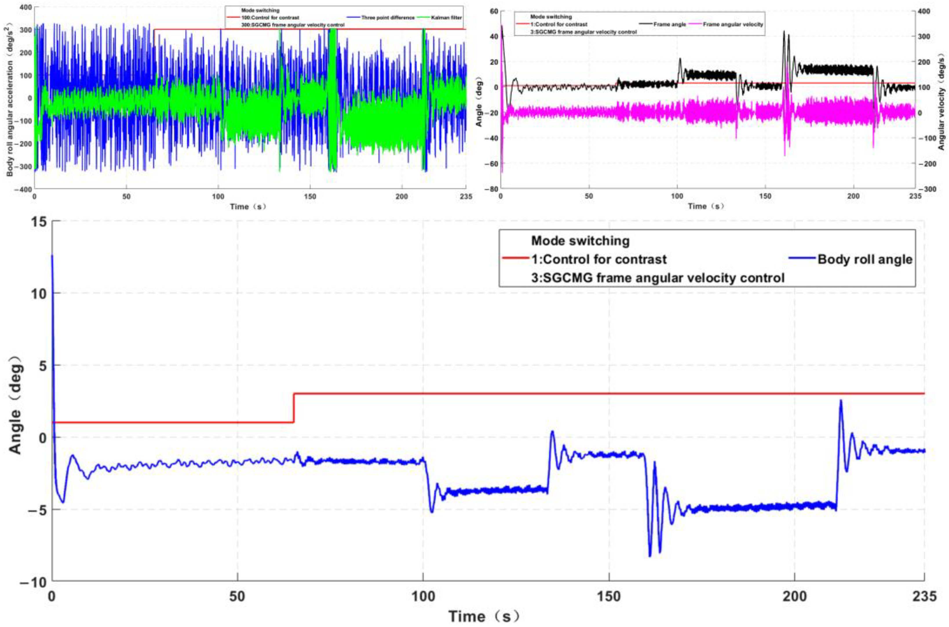
The 10 kg weights were placed at 100 s, the 10 kg weights were removed at 135 s, the 20 kg weights were placed at 159 s, and the 20 kg weights were removed at 211 s. From Figure 19, it can be seen that the equilibrium angles of the car body when placing 10 kg and 20 kg weights are about −3.2° and −4.7°, respectively, the convergence times are about 6 s and 11 s, respectively, and the overshoot amounts are −1.5° and −3.6°, respectively, and the Gravity change of the angle corresponds to the load masses of 12 kg and 20.7 kg, respectively, which are consistent with the actual working conditions. The car body generates a large enough precession moment to control the car body to move in the direction opposite to the external force at the moment the load is placed, and the frame only finds the current car body balance angle at 20° and 40°, which is consistent with the simulation results, and fully proves that the controller has a substantial optimization of real time, response time and resistance to continuous disturbance compared with the controller based on $\dot{\mathsf{\theta }}$, θ feedback. However, it should be noted that the frame does not return to zero when the vehicle is subjected to continuous disturbance. This is due to the static difference in the ${\ddot{\mathsf{\theta }}}_{\mathrm{KF}}$ as mentioned above using the dynamics model as the a priori value without adding the integration link, and this static difference affects the dynamic performance of the SGCMG frame angular velocity controller to some extent. In summary, the effectiveness and advantages of the SGCMG controller designed in this paper have been proved in practical applications.

6. Conclusions

Based on the dynamics modeling and analysis of the two-wheeled motorcycle equipped with SGCMG, this paper proposes the design of a SGCMG frame angular speed control method based on $\ddot{\mathsf{\theta }},\dot{\mathsf{\theta }}$ feedback. The simulation results show that the motorcycle can achieve self-balancing with load under static conditions and stable motion and steering under dynamic conditions. At the same time, the controller has good robustness and stability. Its real-time control effect on the embedded system also demonstrates the effectiveness of the controller when the vehicle is under static with load conditions. In addition, we also compared two controllers based on different feedback data and analyzed their different characteristics, which proved that the controller has good real-time, response speed, and anti-interference ability. At the same time, the Kalman filtering process of $\ddot{\mathsf{\theta }}$ is carried out in this paper, which greatly optimizes the quality of $\ddot{\mathsf{\theta }}$ signal and makes up for the problems of existing sensors.

In the future, we intend to further optimize the $\ddot{\mathsf{\theta }}$ signal quality by replacing the sensor, introducing a time series model in the Kalman filter, and using other methods such as adaptive Kalman filtering. And also consider significantly improving the efficiency of the SGCMG (increasing the rotor speed and the maximum angular velocity of the frame) to ensure that a large enough precession moment is generated to control the stability of the body. Finally, based on the controller designed in this paper, we intend to introduce fuzzy control, adaptive parameter adjustment, and other methods to optimize the control effect, and carry out various dynamic tests to fully verify the effectiveness of the controller, in order to prepare for the real implementation of motorcycle autopilot.