Article

Intelligent-PID with PD Feedforward Trajectory Tracking Control of an Autonomous Underwater Vehicle

1
Department of Mechatronics Engineering, Kocaeli University, Kocaeli 41001, Turkey
2
Department of Mechanical Engineering, Istanbul Technical University, Istanbul 34469, Turkey
*
Author to whom correspondence should be addressed.
Machines 2023, 11(2), 300; https://doi.org/10.3390/machines11020300
Submission received: 19 January 2023 / Revised: 6 February 2023 / Accepted: 16 February 2023 / Published: 17 February 2023
(This article belongs to the Special Issue Control and Mechanical System Engineering)

Abstract

:
This paper investigates the model-free trajectory tracking control problem for an autonomous underwater vehicle (AUV) subject to the ocean currents, external disturbances, measurement noise, model parameter uncertainty, initial tracking errors, and thruster malfunction. A novel control architecture based on model-free control principles is presented to guarantee stable and precise trajectory tracking performance in the complex underwater environment for AUVs. In the proposed hybrid controller, intelligent-PID (i-PID) and PD feedforward controllers are combined to achieve better disturbance rejections and initial tracking error compensations while keeping the trajectory tracking precision. A mathematical model of an AUV is derived, and ocean current dynamics are included to obtain better fidelity when examining ocean current effects. In order to evaluate the trajectory tracking control performance of the proposed controller, computer simulations are conducted on the LIVA AUV with a compelling trajectory under various disturbances. The results are compared with the two degrees-of-freedom (DOF) i-PID, i-PID, and PID controllers to examine control performance improvements with the guaranteed trajectory tracking stability. The comparative results revealed that the i-PID with PD feedforward controller provides an effective trajectory tracking control performance and excellent disturbance rejections for the entire trajectory of the AUV.

1. Introduction

With the increasing interest of scientific researchers and industries in the underwater world, autonomous underwater vehicle (AUV) systems have gained great importance due to their potential to substantially reduce the possible risks and operational costs of underwater missions. Since the technologies working with the data infrastructure have become widespread, underwater vehicles that can perform data collection and underwater observation tasks without the need for human intervention have become essential devices for both commercial and scientific uses.
A fully autonomous vehicle must include guidance, navigation, and control (GNC) software. GNC software architecture refers to the design and organization of software used for the control and navigation of autonomous systems such as AUVs, robots, and spacecraft. GNC software architecture typically includes modules for trajectory planning, state estimation, guidance and control, and monitoring and fault detection [1,2]. Additionally, autonomous vehicles are often capable of performing multiple missions through their multi-mission management software which increases the flexibility and versatility of the system and allows it to perform a wider range of tasks than a single-mission system [3,4]. In this study, the main focus will be on designing a novel model-free trajectory tracking controller for AUV systems.
The unpredictable, complex, and disruptive nature of the underwater environment, along with the highly non-linear and cross-coupled system dynamics, causes disturbances and uncertainties that must be considered in the AUV controller design. In order to perform successful autonomous missions in the underwater environment, a trajectory tracking control system must be utilized in the AUV system, with high precision, satisfactory disturbance rejection, fault tolerance, and robustness properties.
The conventional PID controller is frequently employed by AUV applications, including commercial and scientific uses, due to its simple and effective structure [5,6,7,8]. Despite the cost-effectiveness and implementation simplicity of the PID algorithm, its control performance degradation, especially when the plant is highly non-linear and threatened by the various environmental disturbances, has been reported by numerous studies. Hence, more robust control algorithms are often preferred to guarantee the stable performance and robustness of the controllers. Sliding-mode control has become one of the most favorable non-linear control algorithms for use in the AUV system due to its insensitivity against model uncertainties and external disturbances. Kim et al. [9] proposed an integral sliding-mode controller to stabilize the AUV suffering from the model uncertainties and unknown environmental disturbances, whereas Garcia et al. [10] proposed a model-free high order sliding-mode controller with finite-time convergence and compared it to the regular PID controller. Duan et al. [11] formulated the Hamilton–Jacobi–Isaac equation for the AUV trajectory tracking problem, and designed a reinforcement learning-based model-free controller to obtain optimal trajectory tracking performance. Negahdaripour et al. [12] introduced a sliding-mode controller based on estimated hydrodynamic coefficients. Santos et al. [13] used the instantaneous power data provided by the propulsion system to tune the backstepping sliding-mode controller to achieve energy efficiency and robust movement on the vehicle. Liang et al. [14] designed a novel nonlinear backstepping technique based on the virtual control variables. Gong et al. [15] designed a cascaded control loop wherein backstepping control is designed for the outer loop and a neural network controller is used in the inner loop to solve optimal trajectory tracking control problems of AUV systems. The model of predictive control has been extensively studied for AUV systems in the literature due to its robustness and good handling of nonlinearities [16,17,18]. Shen et al. [19] developed a novel Lyapunov-based model predictive controller framework by utilizing online optimization to enhance trajectory tracking performance in the presence of environmental disturbances, and demonstrated the results comparatively. In order to relieve the so-called chattering phenomenon of the control input of the AUV in the presence of the environmental disturbance and the initial tracking error, Liu et al. [20] proposed a trajectory tracking control strategy based on a virtual closed-loop system. The virtual closed-loop system is used to generate a virtual reference trajectory for the AUV to follow instead of the originally desired trajectory in this study. Additionally, they stated that the new design achieved obvious enhancements in terms of the smoothness of the control input and trajectory tracking precision when measurement noise is considered.
The model-free intelligent-PID control algorithm proposed by Fliess and Coin [21] uses continuously updated local modeling via the unique knowledge of the input–output behavior in order to contribute to the control law used within. Therefore, it can handle the non-linear, cross-coupled, and unmodeled dynamics of the controlled system without the need for information about the plant parameters. That property makes the model-free control a superior option to utilize on AUV control systems. The idea behind developing the proposed i-PID with PD feedforward controller is improving the model-free i-PID control proposed in [21] to have better trajectory tracking precision, external disturbance rejections, and initial tracking error compensations and therefore to overcome the disruptive nature of the underwater environment. The model-free i-PID control algorithm has been implemented in various applications in the literature since it was first introduced. Barth et al. [22] designed a model-free control algorithm based on the model-free control technique proposed by [21] to stabilize the entire flight envelope, including vertical take-off, landing, transition, and forward flight of hybrid UAVs. Effective control performance of the model-free i-PD controller for the entire flight envelope and excellent disturbance rejections during the critical flight phases are reported in this study. Agee et al. [23,24] designed a model-free i-PI controller to solve the trajectory tracking problem of the flexible robot manipulators. Baciu and Lazar [25] presented a new method for tuning i-PID controllers based on an iterative feedback tuning method, and they experimentally evaluated the performance of an i-PID controller tuned by the presented method. Since the high-fidelity modeling of an AUV is a challenging process due to the complex and unpredictable operating environment, model-free control techniques are expected to become more popular in the underwater robotics field in the near future.
In this paper, a model-free i-PID control approach is developed for AUVs, and an i-PID with a PD feedforward (2 DOF i-PID) controller structure is constructed that utilizes the extra PD feedforward controller on all six motion axes to achieve better disturbance rejections and initial tracking error compensation. However, due to the high cross-coupling in the internal dynamics of the AUV system, utilizing the extra PD feedforward loop on all six motion axes causes trajectory tracking precision loss, especially on the orientation axes. Therefore, a novel hybrid controller is developed by combining the i-PID with PD feedforward and i-PID controllers for AUVs to solve the trajectory tracking problem. The proposed hybrid controller framework utilizes the i-PID with PD feedforward controller on the linear motion axes ( x ,   y ,   z ), and the i-PID controller on the angular motion axes ( Φ ,   θ ,   Ψ 
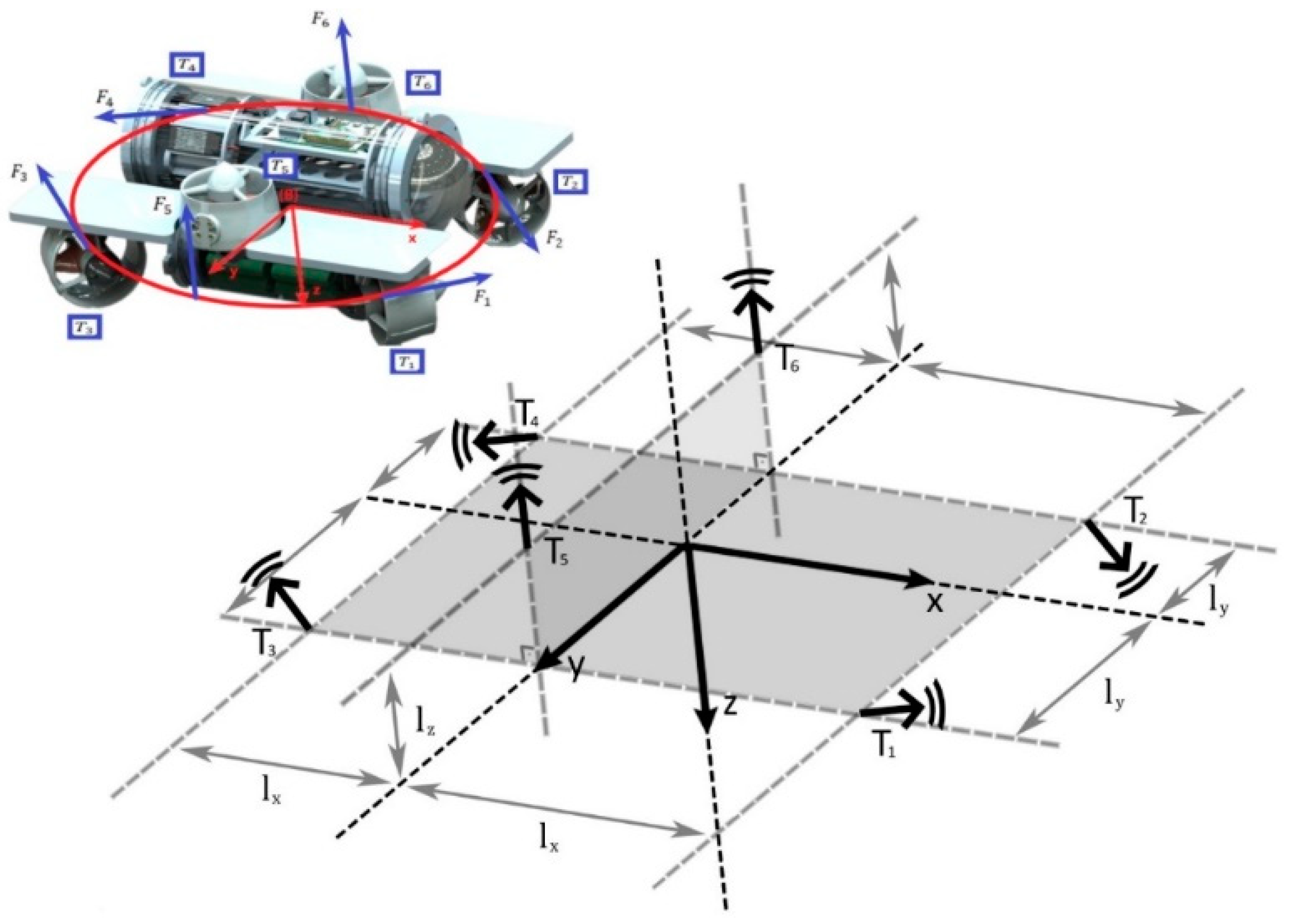
). Since it does not involve a feedforward loop in the angular motion controllers, it can maintain angular trajectory tracking precision while taking the advantages of the extra feedforward controller in the presence of external disturbances and cross-coupled dynamics. The mathematical derivation of the hybrid controller is presented. A mathematical model involving the ocean current dynamics of an AUV is derived in order to obtain better fidelity when investigating ocean current effects, and a model-based ocean current observer is utilized for improving the control performance of the controller against ocean currents. The thruster identification process is addressed, and a transformation matrix between the thruster space and operational space is derived to achieve optimum thrust generation and distribution on the LIVA AUV system. The tuning parameters of the proposed controllers are optimized as described in [26] under several constraints by performing constrained optimization using a nonlinear programming solver such as fmincon in the MATLAB optimization toolbox. The trajectory tracking control performance of the new design is comparatively examined in terms of robustness, tracking precision, disturbance rejection, and energy consumption by conducting computer simulations in the presence of various disturbances and conditions, including worst-case scenario. In order to indicate the maneuvering performance of the new design, a compelling trajectory is also preferred. The proposed hybrid controller performance is compared with the 2 DOF i-PID, i-PID and PID controllers, and the results are discussed. The main contributions of this paper are summarized as follows.
  • The model-free i-PID control approach is developed for the AUVs in the existing literature.
  • The 2 DOF i-PID controller framework is constructed for the trajectory tracking control of autonomous vehicles.
  • A novel model-free hybrid controller design is proposed. The tracking precision, disturbance rejection, and robustness properties of the tracking control are significantly improved, and trajectory tracking stability is guaranteed with the new design.
The paper is organized as follows. In the section “Mathematical Model”, an AUV mathematical model is derived, a model-based ocean current observer is designed and a transformation matrix between the operational space and thruster space is formulated for the LIVA AUV. In the section “Control Strategy”, the control strategy is briefly described, the model-free i-PID controller development is addressed, and a novel hybrid control framework is proposed. In the section “Results and Performance”, the simulation results are discussed in detail. Finally, the conclusions are given in the last section.

2. Mathematical Model

The mathematical model of an AUV can be examined in two separate parts as kinematics and dynamics. Kinematics considers the geometrical transformations of motion, while dynamics analyzes the forces and moments causing motion. Two reference frames in Figure 1 are utilized to define the six-DOF equations of motion of the AUV. The earth-fixed (NED) reference frame is defined relative to the Earth’s reference ellipsoid, and can be represented by   { n } = ( x n ,   y n ,   z n ) and origin  o n [27]. The body-fixed (body) reference frame is a moving coordinate frame that is fixed to the craft and can be represented by   { b } = ( x b ,   y b , z b ) and origin  o b .

2.1. Kinematics

The motions of the AUV are represented by using the SNAME notation [28], where the body frame velocity vector defined as  v = [ υ b / n b   ω b / n b ] T , and where  υ b / n b = [ u   υ   w ] T   is the body frame linear velocity vector and  ω b / n b = [ p   q   r ] T is the body frame angular velocity vector. The position and orientations in the NED frame are defined as  η = [ p b / n n   Θ n b ] T , where  p b / n n = [ N   E   D ] T is the position and  Θ n b = [ Φ   θ   Ψ ] T is the orientation vector [27].
The linear velocity transformation can be performed between the NED and body frames by using (1).
p ˙ b / n n = R b n ( Θ n b ) υ b / n b
R b n ( Θ ) is the linear motion transformation matrix, defined as follows:
R b n ( Θ ) = [ c Ψ c θ s Ψ c Φ + c Ψ s θ s Φ s Ψ s Φ + c Ψ c Φ s θ s Ψ c θ c Ψ c Φ + s Φ s θ s Ψ c Ψ s Φ + s Ψ c Φ s θ s θ c θ s Φ c Φ c θ ]
where  c = cos and   s = sin . The angular velocity transformation can be performed between the NED and body frames as follows:
Θ ˙ n b = T Θ ( Θ n b ) ω b / n b
where  T Θ ( Θ ) is the angular motion transformation matrix, defined as follows.
T Θ ( Θ ) = [ 1 sin Φ tan θ cos Φ tan θ 0 cos Φ sin Φ 0 sin Φ / cos θ cos Φ / cos θ ]
Using (1), (2), (3), and (4), the six-DOF kinematic equations can be expressed in vectorial form as follows [27]:
η ˙ = J ( η ) v
[ p ˙ b / n n Θ ˙ n b ] = [ R b n ( Θ n b ) 0 3 × 3 0 3 × 3 T Θ ( Θ n b ) ] [ υ b / n b ω b / n b ]

2.2. Dynamic Model

The six-DOF dynamic equations of the AUV subject to ocean current disturbance are expressed via the laws of Newton as follows [29]:
M R B v ˙ + C R B ( v ) v = τ H
τ H = M A v ˙ C A ( v r ) v r D ( v r ) v r g ( η ) + τ c
where  τ c is the control torque input,  v r = v v c b   is the relative velocity of the vehicle and  v c b is the ocean current velocity defined in the body frame.  M R B is the rigid body mass matrix,    C R B is the rigid body Coriolis and Centripetal matrix due to the rotation of body frame about the NED frame, and  M A and  C A are the added mass matrix and the hydrodynamic Coriolis matrix, respectively. The hydrodynamic damping effects applied to the AUV are captured by the matrix  D , which includes linear and quadratic damping terms. The restoring forces and moments applied on the AUV are captured by the term  g ( η ) , and consist of two elements called gravitational forces and buoyancy forces. The gravitational forces ( W ) act through the center of gravity whereas the buoyancy forces ( B ) act through the center of buoyancy. The AUV is designed such that the buoyancy forces are slightly larger than the gravitational forces (i.e.,  B > W ), to make the vehicle surface in the event of an emergency. Additionally, a distance between the center of gravity and center of buoyancy is left in the structural design of AUV to naturally contribute to the control of the roll  ( Φ ) and pitch ( θ ) axes. Considering the underactuated AUV, this property is important for stabilizing the vehicle in the presence of nonlinearities in the environment and the AUV itself [29]. The hydrodynamic forces are derived in (8) by assuming ocean current velocity is constant (i.e.,    v ˙ c n 0 ) in the NED frame. However, even though the ocean current velocity is assumed constant in the NED frame, the rotational motions of the AUV lead to a correspondingly changing body-fixed current velocity (i.e.,  v ˙ c b 0 ). Therefore, the acceleration of the ocean current induces a force on the AUV, which is captured by the term  A c ( v c b ) v r in the dynamic Equation (13).
The ocean current speed magnitude  V c and its relative direction to the moving object are conveniently expressed in terms of angle of attack   α c and sideslip angle   β c . Thus, a 3-D irrotational ocean current vector  v c n can be formulated relative to the NED frame as follows [27].
v c n = [ V c cos ( α c ) cos ( β c ) V c sin ( β c ) V c sin ( α c ) cos ( β c ) 0 3 × 1 ]
The ocean current vector in the NED frame  v c n can be transformed to the body frame, using the kinematic equation derived previously, for use in the dynamic equations of the AUV as given in (10).
v c b = d i a g [ R b n T ( Θ ) , 0 3 × 3 ] v c n
The acceleration of the ocean currents in body frame  v ˙ c b can be derived by defining [29]:
S ( ω b / n b ) = [ 0 r q r 0 p q p 0 ] = S T ( ω b / n b )
where  S is the skew-symmetric vector cross-product matrix. Thus, the following relation can be defined [29]:
v ˙ c b = S c ( ω b / n b ) v c b
where  S c ( ω b / n b ) = d i a g [ S ( ω b / n b ) , 0 3 x 3 ] = S c T ( ω b / n b ) . Hence,  M A v ˙ c b = M A S c ( ω b n b ) v c b , and  A c ( v c b ) v r   M A S c ( ω b / n b ) v c b [29]. The final dynamic equation including ocean currents becomes:
M v ˙ + C R B ( v ) v = C A ( v r ) v r D ( v r ) v r g ( η ) + A c ( v c b ) v r + τ c
M = M A + M R B

2.3. Ocean Current Observer

The model-based ocean current observer proposed by Borhaug et al. [30] is adapted for the AUV model to estimate unknown ocean current velocity  v c b with the help of the knowledge of the dynamical model and availability of the control torque input   τ c , AUV velocities  v and the orientation angles   Θ [30].
M v ^ ˙   = C R B ( ν ) ν g ( η ) + τ ^ H + τ c + K 1 ( v v ^ )
v ^ c ˙ = S c ( ω ) v ^ c b + K 2 ( v v ^ )
where  K 1 and  K 2 are observer gain matrices,  v ^ is the estimation of the vehicle velocity and  v ^ c b is the estimation of the ocean current velocity. The hydrodynamic term in the observer model including ocean current velocity estimation becomes the following:
τ ^ H = C A ( v ^ v ^ c b ) ( v ^ v ^ c b ) D ( v ^ v ^ c b ) ( v ^ v ^ c b ) + A c ( v ^ c b ) ( v ^ v ^ c b )

2.4. Experimental Platform

As an experimental platform, all simulations were carried out on LIVA AUV [31] shown in Figure 2 and it was developed at the Robotics and Automation Laboratory of the Mechatronics Engineering Department at Kocaeli University.
The mathematical model parameters of the LIVA AUV that were used in the computer simulations are listed in Table 1. The linear motion axis position information ( x ,   y ,   z )   is obtained through a mapping algorithm which uses the onboard camera data to calculate position data of the vehicle with respect to the predefined pool map. The angular motion axis orientation information ( Φ ,   θ ,   Ψ ) is measured by using onboard IMU sensor which utilizes an internal extended Kalman filter algorithm to improve information precision. The LIVA AUV is capable to perform autonomous target-following missions through its onboard computer, which utilizes an online image processing and trajectory generation algorithms to track the predefined object in the pool.

2.5. Thruster Identification

The correlation between the thrust force produced by a single thruster in the steady state and the corresponding PWM duty cycle given to the electronic speed controllers (ESCs) must be identified to derive a thruster model. The derived correlation will then be used to map control signals to the corresponding thrust forces in the thruster model. A testing setup shown in Figure 3 was prepared to measure the produced thrust forces under varying PWM duty cycles. The instantaneous current drawn by the thruster motor has also been measured to identify the most efficient operating range of the thruster in order to achieve the smallest possible energy consumption by the vehicle.
The produced thrust forces are calculated by using (18) after the measuring process is complete.
F T 1 l 1 = F m e a s u r e d l 2
After all the thrust forces are computed for the corresponding PWM duty cycles, the thrust force, PWM duty cycle, and the instantaneous current drawn from the battery by the motor chart are derived as shown in Figure 4.
The thrust force fluctuation of PWM duty cycles within the range of 85% to 98% might stem from both the nonlinearities of the drive components (i.e., battery, ESCs and BLDC motors) and the measurement errors. According to the revealed correlation between the current consumption and force production of the propeller, the maximum thrust force produced by a single thruster in the efficient range is determined approximately as  40 Newtons. Considering that the AUV has six identical thrusters and the thrust coefficients for individual thrusters are defined as  K T 1 −  K T 6 , the thruster coefficient matrix is derived as follows.
K T = d i a g [ K T 1   K T 2   K T 3   K T 4   K T 5   K T 6 ]

2.6. Thrust Force Generation Model

The control system of the AUV produces six-DOF control signals relative to the operational space, and the AUV motions are generated by using the six onboard thrusters of the vehicle. A transformation matrix between the operational space and thruster space must be derived to achieve optimum thrust force generation on the AUV system.
The thruster locations and the corresponding force directions in the positive propulsion case are shown in Figure 5.
The control forces and moments produced by the vehicle thruster system can be derived using (21):
i ( x , y , z , Φ ,   θ ,   Ψ )
F T = P 1 K T u i
F T m a x b F T F T m a x f
where  P = [ P 1   P 2   P 3   P 4   P 5   P 6 ]   ϵ   R 6 × 6 is the thruster configuration matrix and  u i is the control input vector produced by the corresponding 6 DOF controller. Since the LIVA AUV contains six thrusters, the thrust force generated by the six thrusters of the AUV can be represented as a vector  F T = [ F T 1   F T 2   F T 3   F T 4   F T 5   F T 6 ] T ϵ   R 6 × 1 , and it is saturated by  F T m a x f and  F T m a x b ,   which are the maximum producible thrust forces by a single thruster in forward and backward directions, respectively.
The control forces and moments demanded by the AUV control system in six DOF can be formulated as follows.
τ c = P F T = P P 1 K T u i = K T u i
The orientation angles of the thrusters  T 1 to  T 4 relative to the z-axis of the body frame are  π 4 , π 4 , 3 π 4 and  3 π 4 , respectively. The derivation of the configuration vector of the thruster  T 1 is as given in (24).
P 1 = [ cos ( π / 4 ) sin ( π / 4 ) 0 sin ( π / 4 ) ( 0.004 ) cos ( π / 4 ) ( 0.004 ) sin ( π / 4 ) l x 1 cos ( π / 4 ) l y 1 ]
where  l x 1 and  l y 1 are the x-axis and y-axis distances of the thruster  T 1 to the center of gravity, respectively. Thus, the thruster configuration matrix P is obtained by calculating the thruster configuration vectors for all six thrusters.

3. Control Strategy

The model-free i-PID controller is developed for all six motion axes of the AUV system based on the model-free control technique proposed by [21], hence it has no information about the AUV plant model (e.g., mass, inertia, hydrodynamic coefficients, etc.). Afterward, the i-PID with PD feedforward (2 DOF i-PID) control framework is constructed by modifying the developed i-PID controller to include an extra PD feedforward loop on all six motion axes in the controller structure. Finally, a novel hybrid controller framework is developed for the AUVs by combining the developed i-PID with PD feedforward and i-PID controllers.
The idea behind developing the novel controller framework is to take the advantages of the disturbance rejection, initial tracking error compensation, and robustness capabilities of the two-DOF control architecture without experiencing loss of precision or instabilities in the cross-coupled and unactuated motion axes. In the novel controller framework, the linear motion axes ( x ,   y ,   z ) of the AUV are controlled by the three i-PID with PD feedforward controllers, and the angular motion axes ( Φ ,   θ ,   Ψ ) are controlled by the three i-PID controllers.

3.1. Model-Free i-PID Controller Design

Writing reliable differential equations for mathematically representing a plant model is always difficult and time-consuming. To summarize the main theoretical idea that the model-free control is based on, the model-free control uses continuously updated local modeling via unique knowledge of the input–output behavior instead of using complex differential equations [21].
Assuming that the relationship between the inputs and outputs of a given system is represented by an unknown finite order differential equation, in the model-free approach, this mathematical model is represented by a structure called the ultra-local model, which is only valid during very short time intervals [21].
y ( h ) = F + a u
Parameter h is the derivation order which is greater than or equal to 1, and a is the non-physical constant parameter. F is the quantity representing the real dynamics of the AUV as well as the external disturbances for each axis of six DOF. Hence, the accurate estimation of the F, defined as  F ^ , has great importance for achieving better model-free control performance. The numerical value of F at any time instant is estimated by using the constant a, control input u and the output  y ( h ) . Assuming h = 2 in (25) yields:
F ^ ( t ) = y ¨ ( t ) a u ( t )
Then, closing the loop via an intelligent PID, we obtain:
u ( t ) = F ^ ( t ) a + y * ¨ ( t ) a + K P e ( t ) + K I   e ( t ) + K D e ˙ ( t )
where:
  • y* is the reference trajectory,
  • e = yy* is the tracking error, and
  • KP, KI, KD are the controller tuning gains.
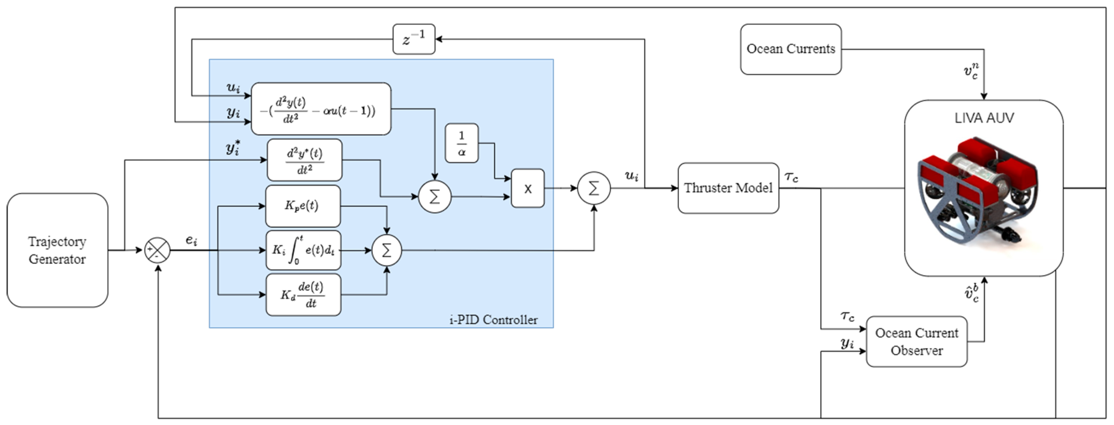
The block diagram representation of the developed i-PID controller structure is given in Figure 6 to represent the key concepts of the model-free i-PID control approach visually.
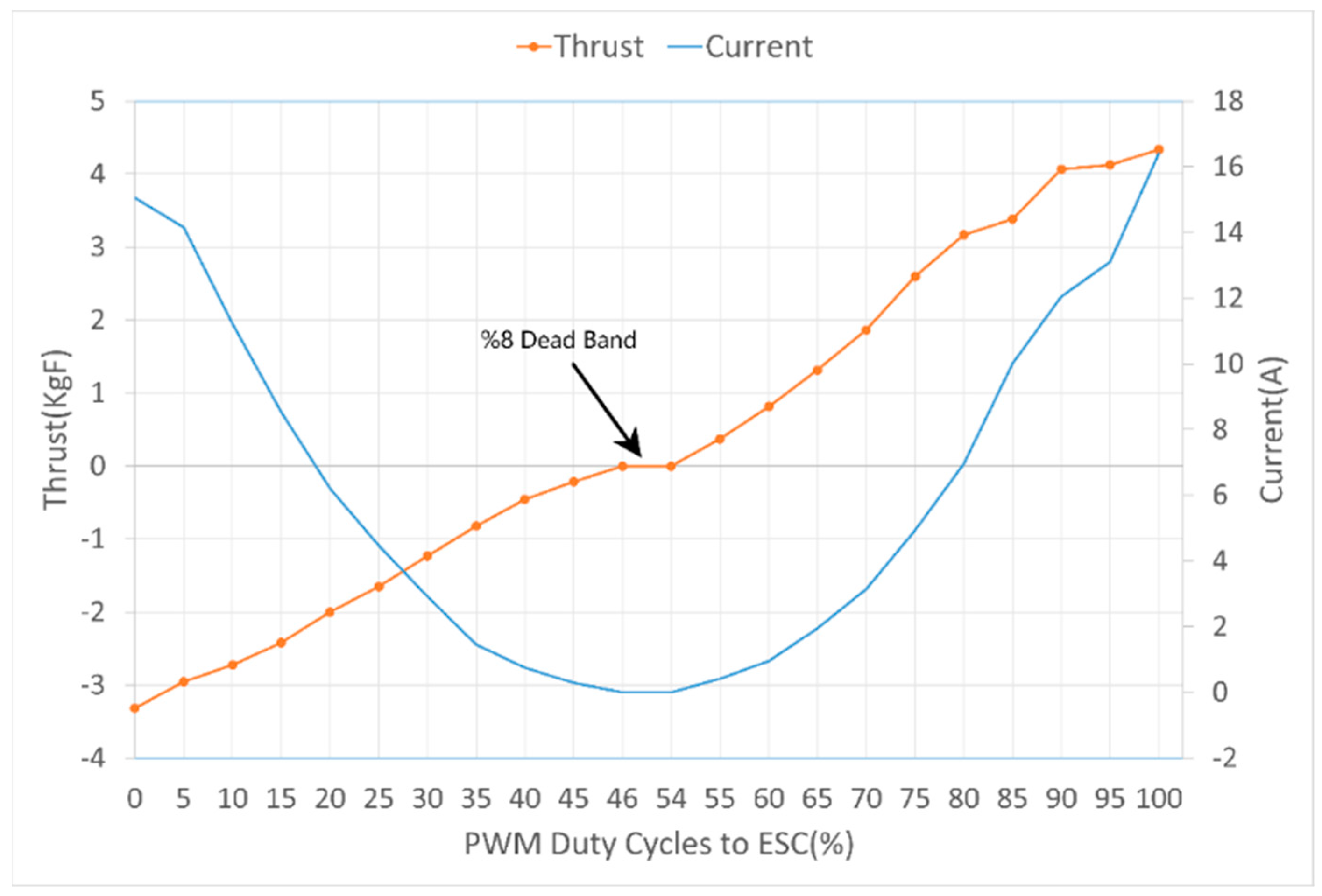
In the real-time implementation of the proposed control architecture, the trajectory generation, trajectory tracking control, ocean current observer and thruster model subsystems are on the software level. The force demands obtained by using (21) in the thruster model subsystem are converted into PWM signals using the chart in Figure 4, and sent directly to ESCs of the thruster motors which are on the hardware level, to produce required torques and moments. The explained relation applies for all controller structures in this paper.

3.2. i-PID with PD Feedforward (2 DOF i-PID) Controller Design

Utilizing an extra feedforward loop in the trajectory tracking controller structure is a very common method in the literature [26,32,33], especially when high external disturbances are present in the operating environment. The main idea of using the feedforward structure in trajectory tracking control is enhancing the strength of the feedback system against external disturbances and model uncertainties using a feedforward controller.
The PD feedforward control law can be derived for a SISO system as follows:
G ( t ) = α K P y * ( t ) β K D y * ˙ ( t )
where  α and  β are the feedforward controller tuning parameters. Combining (27) and (28) yields the complete i-PID with PD feedforward control law. The control law is then extended by defining six SISO controllers for six motion axes of the AUV. Finally, the i-PID with PD feedforward controller is derived as follows for six-DOF AUV motion control.
u i ( t ) = F ^ i ( t ) a i + y * ¨ i ( t ) a i + K P i e i ( t ) + K I i   e i ( t ) + K D i e ˙ i ( t ) + G i ( t )
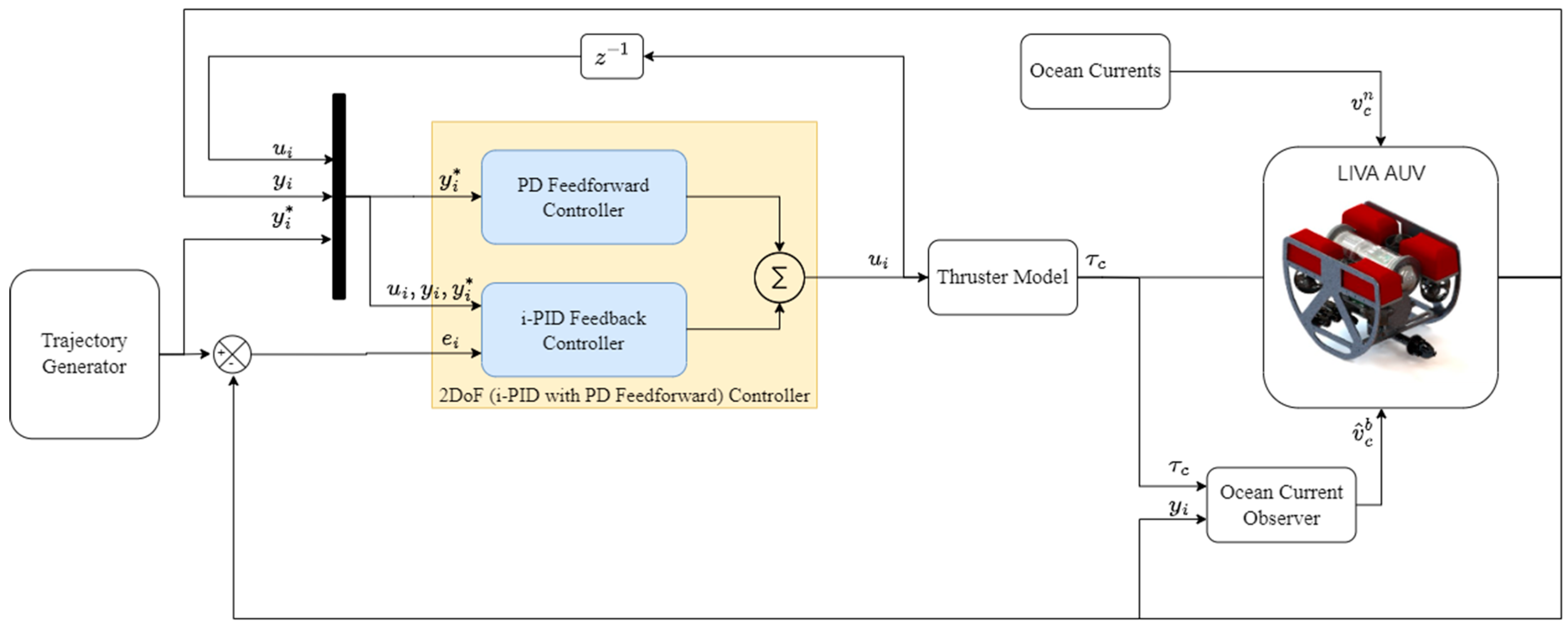
The developed control structure is summarized in Figure 7.

3.3. Hybrid Controller Design

An underwater vehicle encounters many different forces and disturbances when operating in the underwater environment; these are generally unexpected and nontrivial to mathematically represent. Therefore, considering these forces and disturbances to achieve robust and stable motions of the AUV becomes a must. However, obtaining these forces experimentally is a difficult and expensive process.
The proposed hybrid controller framework is developed to satisfy the trajectory tracking control requirements of the AUV system in the presence of the disruptive conditions of the underwater environment. Since the proposed control algorithm has no information about the plant and external disturbances, the possible expenses of plant modelling and experimenting with the external forces of the underwater environment are saved. The proposed hybrid i-PID controller structure consists of two subparts as the position  ( x ,   y ,   z ) , and the orientation ( Φ ,   θ ,   Ψ ) controllers. The position controller consists of the three i-PID with PD feedforward controllers which employ the i-PID controller as a feedback controller and the conventional PD controller as a feedforward controller. The feedforward structure provides better disturbance rejections on the axes wherein the motion generation is desired. Additionally, the axes on which the motion generation is undesired must be kept stable on the AUV to avoid the system becoming unstable. The instability avoidance problem becomes more crucial when considering that the Euler transformation used in the kinematic equations involves singular points in its internal mathematics which must be avoided during operations. Hence, the feedforward structure is not employed in the orientation controller of the hybrid design to achieve better overall trajectory tracking precision and to reduce the total tuning parameter number on the system. Consequently, the orientation controller consists of the three i-PID controllers. 
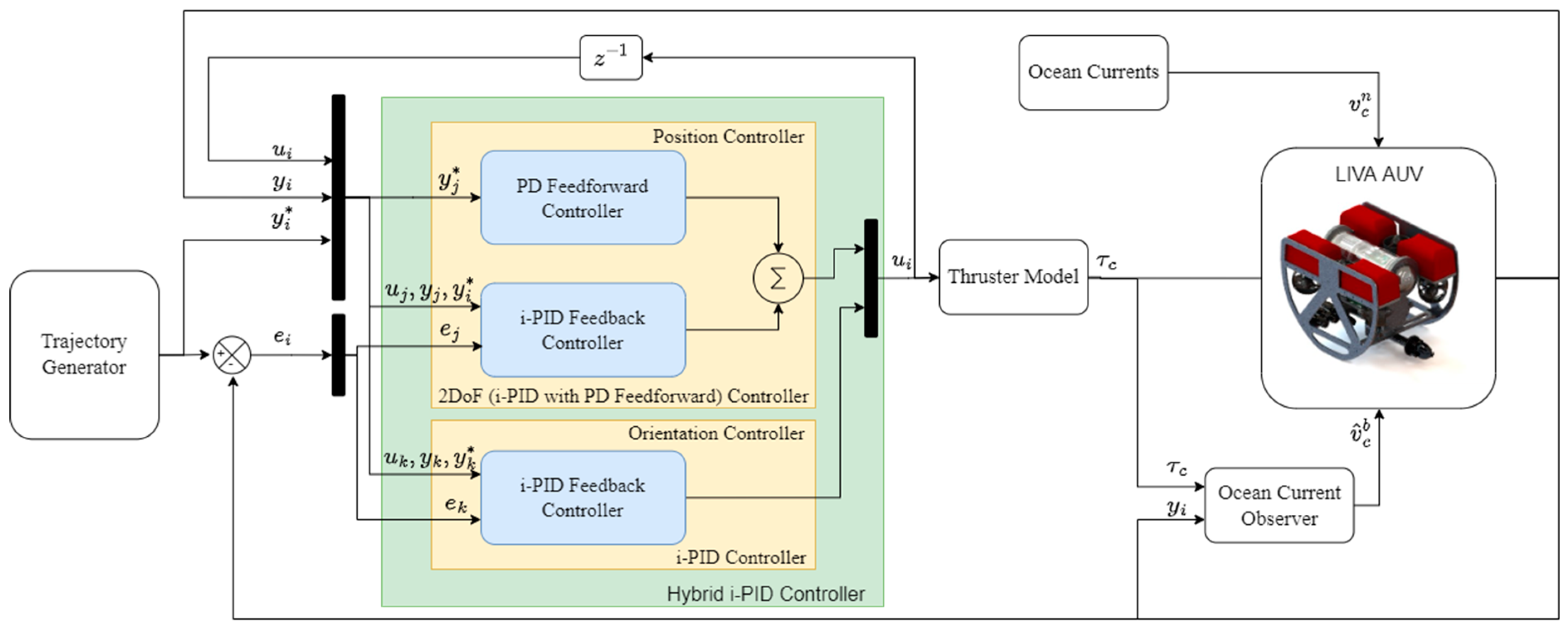
Figure 8 shows the main ideas of the proposed hybrid control architecture.
Considering the model-free control algorithms have been developed for single-input–single-output (SISO) systems and the LIVA AUV has been modelled by six inputs (6 thrusters) and six outputs ( x ,   y ,   z , Φ ,   θ ,   Ψ ), the proposed hybrid control architecture comprises six SISO controllers.
The linear motion axes PD feedforward input  G j ( t ) can be defined as follows:
G j ( t ) = α j K P j y * j ( t ) β j K D j y * ˙ j ( t )
where  j ( x ,   y ,   z ) . Combining (27) and (30) yields the complete i-PID with PD feedforward control law   u j   for the linear motion axes  ( x ,   y ,   z ) as follows:
u j ( t ) = F ^ j ( t ) a j + y * ¨ j ( t ) a j + K P j e j ( t ) + K I j   e j ( t ) + K D j e ˙ j ( t ) + G j ( t )
By utilizing (27), the complete i-PID control law for the angular motion axes  ( Φ ,   θ ,   Ψ ) can be defined by  u k :
u k ( t ) = F ^ k ( t ) a k + y * ¨ k ( t ) a k + K P k e k ( t ) + K I k   e k ( t ) + K D k e ˙ k ( t )
where  k ( Φ ,   θ ,   Ψ ) F ^ j = [ F ^ x , F ^ y , F ^ z ] and  F ^ k = [ F ^ Φ , F ^ θ , F ^ Ψ ] . The resulting  F ^ j , k is the amount representing the sum of the real dynamics of the AUV and external disturbances in each axis of the six DOF. Thus, we can define six-DOF hybrid control law in a vector representation as follows.
U = [ u x   u y   u z   u Φ   u θ   u Ψ ] T

4. Results and Performance

To demonstrate control performance improvement achieved by the novel controller and inspect the resulting behavior under the different conditions and disturbances, the computer simulations were conducted for the PID, i-PID, 2 DOF i-PID, and hybrid controllers. The control inputs and trajectory tracking errors for all controllers are shown, and the tabulated results are discussed individually for all simulation cases in this section.
To evaluate and compare the performances of the controllers, some performance metrics were used. These are the integral of absolute error (IAE), the integral of absolute error multiplied by time (ITAE), the integral of the square of the control input (ISCI), and the integral of variance of the control input (IVCI). The control performance indexes are given in Equations (34)–(37).
I A E = 0 t | e r e a l |   d t
I T A E = 0 t t | e r e a l |   d t
I S C I =   i = 1 6 | u i | 2
I V C I =   i = 1 6 | Δ u i |
where  e r e a l denotes the real tracking error  e r e a l = η r , and   u i denotes the control input produced by the  i t h thruster. The reference trajectory used in the simulations was designed to be the hardest possible trajectory, and includes several maneuvering sequences to analyze controller performances when the torque demand and speed are transiently approaching the physical limits of the AUV.
In computer simulations, the current speed was generated as a random number with  0.5   m / s mean and  ± 0.3   m / s variance. The ocean current angle components   α c and  β c were also generated as a random number with  45   degrees mean and  ± 45   degrees variance. Sampling frequency and simulation times of 1 kHz and 100 s were used, respectively. The additive measurement noise used here was set as zero-mean Gaussian noise, with a maximum amplitude of  ± 0.1   m in position and  ± 2.3   degrees in orientation measurements. The  K 1 and  K 2 observer gain matrices were chosen as  K 1 = ( I + M A + M R B ) K 2 and  K 2 = 2 I 6 × 6 . The thruster limits are defined as  F m a x f F m a x b = 40   N , and the thruster coefficient matrix  as   K T = d i a g [ 40   40   40   40   40   40 ] . The non-physical constant parameter  a in (25) is found by trial and error by conducting computer simulations. The tuning parameters of the controllers, i.e.,  K P K I K D α and  β are found by performing optimization, as described in [26] in the MATLAB optimization toolbox, using a nonlinear programming solver such as the fmincon function.

4.1. Trajectory Tracking Control Simulation

The reference trajectory used in this simulation was defined by  r 1 = [ x d , y d , z d , 0 , 0 , 0 ]   T , where  x d = 2 sin ( 0.096 t ) + 2 sin ( 0.288 t ) y d = 2 sin ( 0.048 t ) + 2 sin ( 0.144 t ) and  z d = 0.1 t 
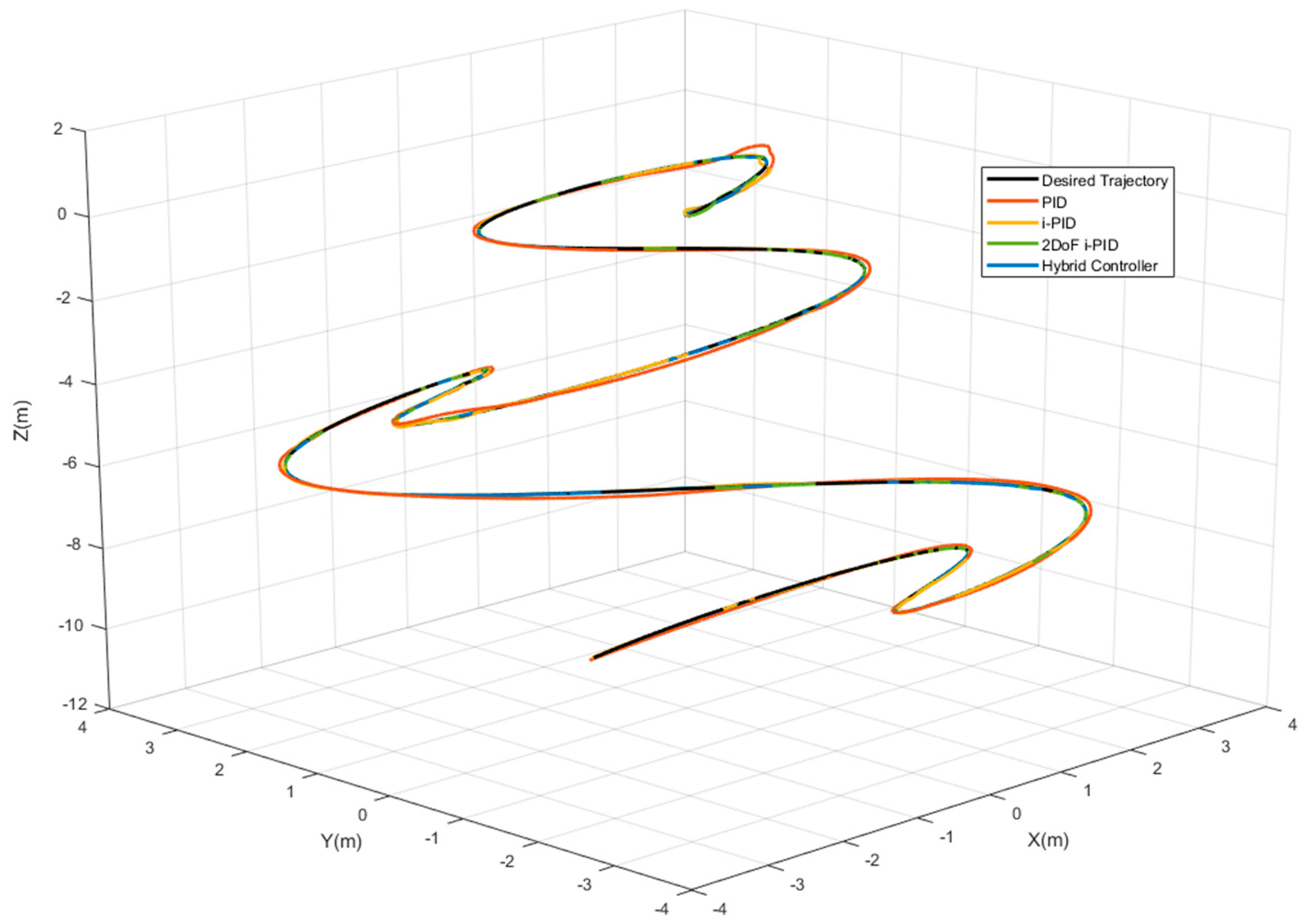
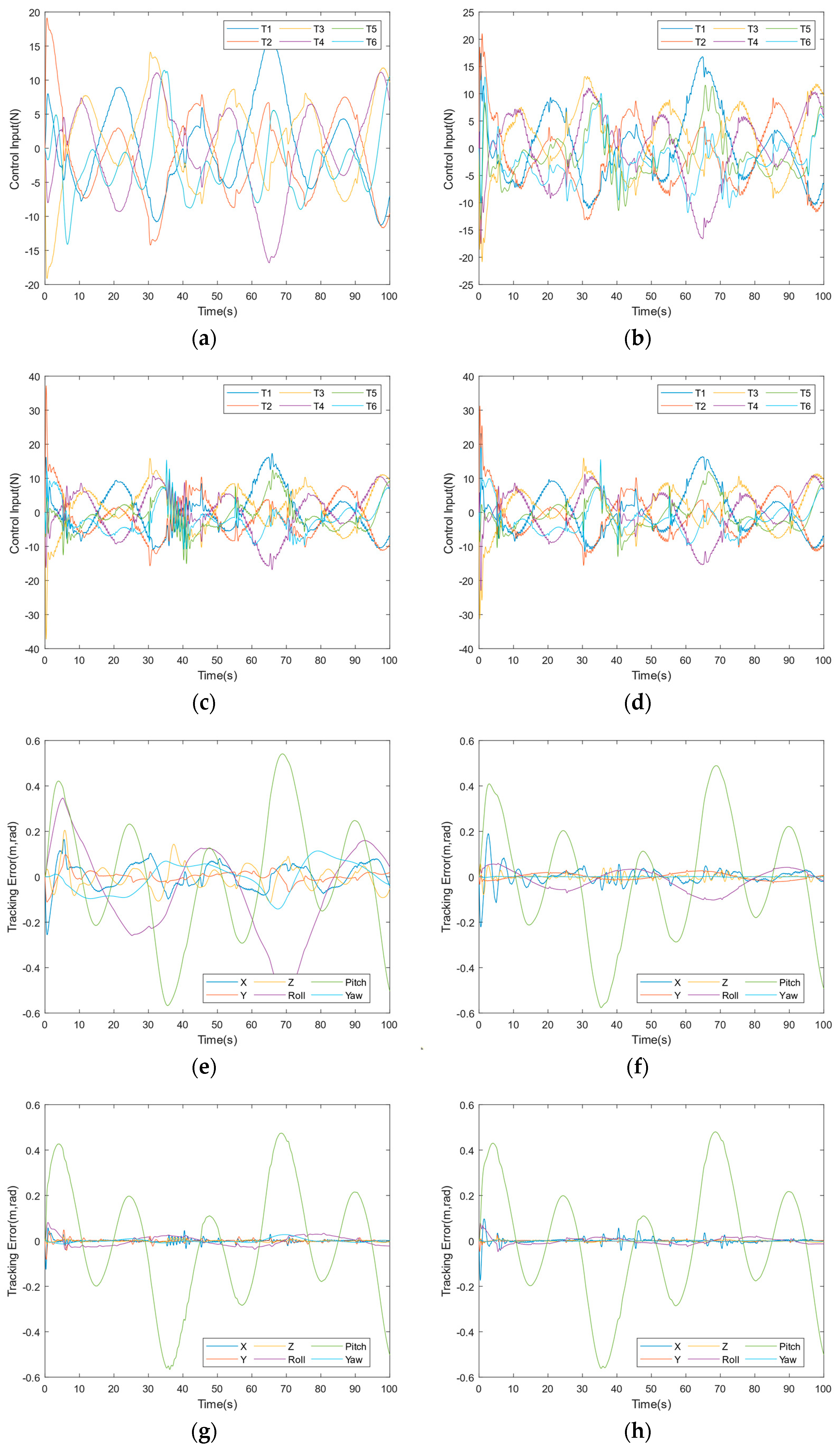
. The trajectory tracking simulation was conducted only in the presence of random ocean currents. The measurement noise, external disturbances, thruster malfunction, and model parameter uncertainty were not considered in this case. The simulation results are given in Figure 9 and Figure 10.
Considering the six-DOF tracking errors along the trajectory, it can be seen that whenever the vehicle tried to accelerate in X or Y axes, the ocean current affected the vehicle behavior heavily, and the i-PID controller was not able to compensate it sufficiently compared to the hybrid and two-DOF i-PID controllers. Nevertheless, the i-PID controller completed the trajectory without a serious deviation. The two-DOF i-PID and hybrid controllers responded to the ocean current effects very well, and the extra feedforward loop provided excellent ocean current disturbance rejection to the vehicle. Additionally, by looking at the control inputs, it can be observed that the controllers including the feedforward loop responded to the initial tracking errors quickly and provided extra initial tracking error compensation to the AUV system. However, as can be seen from Table 2 and the IAE values of the two-DOF i-PID controller, the feedforward loop did not provide a better trajectory tracking precision on the angular motion axes. The tracking precision of the Yaw angle ( Ψ ), which is coupled with the X and Y axes, was significantly corrupted by the extra feedforward loop in the two-DOF i-PID controller. The hybrid controller has the least value in terms of ISCI as can be seen in Table 3, indicating that in the presence of the random ocean current effects, the hybrid controller consumed less energy compared to the other controllers while providing the best overall trajectory tracking precision.

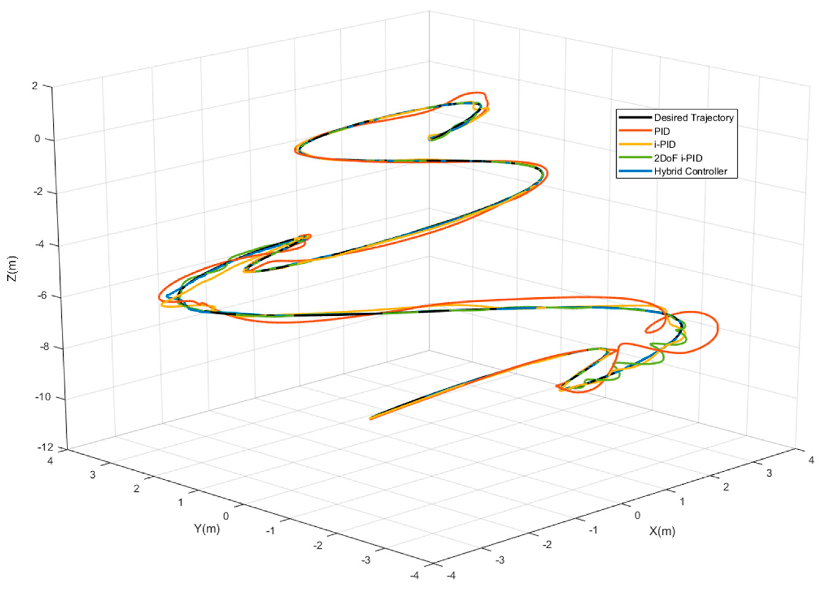
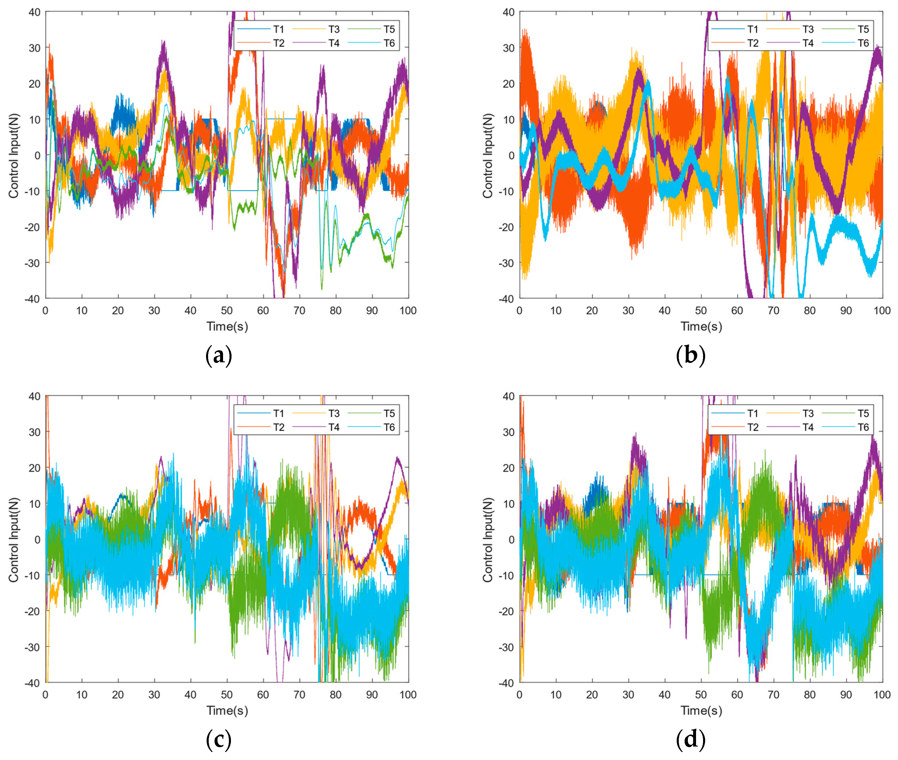
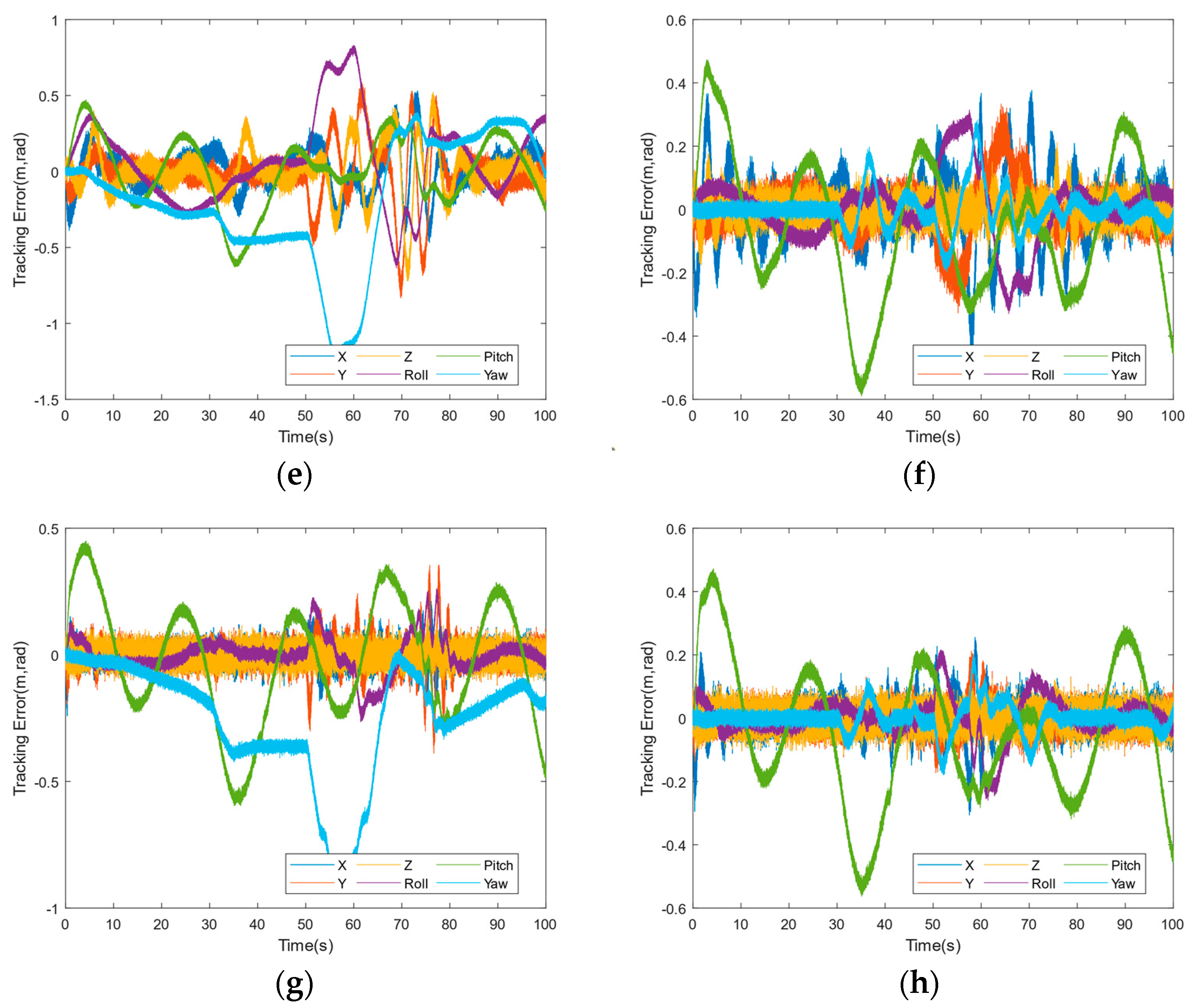
4.2. Worst-Case Trajectory Tracking Control Simulation

The reference trajectory used in this simulation was redefined by  r 2 = [ x d , y d , z d , 0 , 0 , Ψ d ]   T , where  x d = 2 sin ( 0.096 t ) + 2 sin ( 0.288 t ) y d = 2 sin ( 0.048 t ) + 2 sin ( 0.144 t ) z d = 0.1 t and  Ψ d = sin ( 0.016 π t ) . The trajectory tracking simulation was conducted in the presence of the measurement noise, random ocean currents, external disturbances, thruster malfunction and model parameter uncertainty. The external disturbances were applied as  F e x t 1 = [ 0   40 N   0   0   0   0 ]   T impulse disturbance between the 50th and 60th seconds, and  F e x t 2 = [ 0   0   40 N   0   0   0 ]   T step disturbance at the 75th seconds of the simulation. In addition, the thruster  T 1 malfunctioned at the 25th second of the simulation, and its capacity was reduced to 25% of its full range. The 30% model parameter uncertainty was applied, and the measurement noise was also considered. The controller performances are shown in Figure 11 and Figure 12 and the performance measures are presented in Table 4 and Table 5.
Considering the LIVA AUV platform includes cross-coupled motion axes and it is operating in the highly nonlinear underwater environment, generating a stable motion in one axis also contributes to other motion axes and enhances the overall trajectory tracking performance. The main contribution of the hybrid controller to the model-free i-PID control is taking the disturbance rejection and fast initial tracking error compensation advantage of the extra feedforward loop in the linear motion axes without causing any disruption on the coupled angular motion axes. Therefore, it can be seen that hybrid controller achieved better overall tracking performance as expected, and it has the least values in terms of IAE and ITAE, except for the X-axis. As can be seen that the PID and two-DOF i-PID controllers seriously deviated when the external disturbances were applied. The feedforward loop in the angular motions control law of the two-DOF i-PID caused losses of precision even worse than in the first simulation when the Yaw ( Ψ ) motion trajectory tracking is requested. The i-PID controller showed relatively poor continuous tracking precision compared to the other controllers. The two-DOF i-PID controller has the least value in terms of ISCI, meaning that it completed the trajectory with the least energy consumption. Despite the i-PID controller providing smoother control inputs and the two-DOF i-PID consuming less energy than the hybrid controller, the advantages of the hybrid controller in terms of tracking precision and robustness are obvious compared to the other controllers. Additionally, as can be seen in the simulation results, under the cumulative effects of the applied external and internal disturbances to AUV, the hybrid controller achieves much better results. It is important to note that the i-PID control relies heavily on the accurate estimation of  F ^ , so the performance of the model-free control may degrade when  F ^ is not predicted with sufficient accuracy.
The presented controller comparison is visualized using MATLAB/Simulink and Unreal Engine 4 environments; the relevant video can be found in [31].

5. Conclusions

A novel trajectory tracking control framework was developed based on i-PID with a PD feedforward control algorithm for an AUV system in the presence of the ocean currents, external disturbances, measurement noise, model parameter uncertainty, thruster malfunction, and the initial tracking error. The trajectory tracking precision and robustness improvements achieved by the proposed controller were shown with the guaranteed trajectory tracking stability. Ocean current dynamics were included in the mathematical model of the AUV to achieve better fidelity when examining the effects of ocean current, and a model-based ocean current observer was employed to contribute to the performance of the control system. The thruster identification process was addressed, and a transformation matrix between the thruster space and operational space was derived to obtain optimum thrust generation and distribution on the AUV system. Two simulation scenarios were conducted with the PID, i-PID, two-DOF i-PID, and hybrid controllers to examine the trajectory tracking control performance of the new design in the presence of the various disturbances. The comparative results of the simulation on the LIVA AUV system revealed the advantages of the proposed hybrid controller in terms of the trajectory tracking precision and the robustness of the control system. Moreover, the comparative results show that the novel controller design here does not have any considerable disadvantage in terms of the energy consumption. In future works, the simulation results obtained by the proposed controller will be verified experimentally.

Author Contributions

Conceptualization, Z.B.; methodology, Z.B.; software, K.G.; validation, K.G.; formal analysis, K.G.; investigation, Z.B.; resources, K.G.; data curation, K.G.; writing—original draft preparation, K.G.; writing—review and editing, Z.B.; visualization, K.G.; supervision, Z.B.; project administration, Z.B. All authors have read and agreed to the published version of the manuscript.

Funding

This research received no external funding.

Data Availability Statement

Not applicable.

Conflicts of Interest

The authors declare no conflict of interest.

References

  1. Nađ, Đ.; Mišković, N.; Mandić, F. Navigation, guidance and control of an overactuated marine surface vehicle. Annu. Rev. Control 2015, 40, 172–181. [Google Scholar] [CrossRef] [Green Version]
  2. Kondapalli, A.; Nandi, P.; Kaipa, K. Development of a Three-Dimensional Simulator for Integrated Testing of Path-Planners and Controllers for Autonomous Underwater Vehicles. In OCEANS 2022, Hampton Roads; IEEE: New York, NY, USA, 2022; pp. 1–10. [Google Scholar] [CrossRef]
  3. Conte, G.; Scaradozzi, D.; Sorbi, L.; Panebianco, L.; Mannocchi, D. ROS multi-agent structure for autonomous surface vehicles. In OCEANS 2015-Genova; IEEE: New York, NY, USA, 2015; pp. 1–6. [Google Scholar] [CrossRef]
  4. D’angelo, V.; Folino, P.; Lupia, M.; Gagliardi, G.; Cario, G.; Gaccio, F.C.; Casavola, A. A ROS-Based GNC Architecture for Autonomous Surface Vehicle Based on a New Multimission Management Paradigm. Drones 2022, 6, 382. [Google Scholar] [CrossRef]
  5. Khodayari, M.H.; Balochian, S. Modeling and control of autonomous underwater vehicle (AUV) in heading and depth attitude via self-adaptive fuzzy PID controller. J. Mar. Sci. Technol. 2015, 20, 559–578. [Google Scholar] [CrossRef]
  6. Wu, B.; Han, X.; Hui, N. System Identification and Controller Design of a Novel Autonomous Underwater Vehicle. Machines 2021, 9, 109. [Google Scholar] [CrossRef]
  7. Anderlini, E.; Parker, G.G.; Thomas, G. Control of a ROV carrying an object. Ocean Eng. 2018, 165, 307–318. [Google Scholar] [CrossRef]
  8. Chin, C.S.; Lau, M.W.S.; Low, E.; Seet, G.G.L. A robust controller design method and stability analysis of an underactuated underwater vehicle. Int. J. Appl. Math. Comput. Sci. 2006, 16, 345–356. [Google Scholar]
  9. Kim, M.; Joe, H.; Kim, J.; Yu, S.-C. Integral sliding mode controller for precise manoeuvring of autonomous underwater vehicle in the presence of unknown environmental disturbances. Int. J. Control 2015, 88, 2055–2065. [Google Scholar] [CrossRef]
  10. González-García, J.; Gómez-Espinosa, A.; García-Valdovinos, L.G.; Salgado-Jiménez, T.; Cuan-Urquizo, E.; Cabello, J.A.E. Experimental Validation of a Model-Free High-Order Sliding Mode Controller with Finite-Time Convergence for Trajectory Tracking of Autonomous Underwater Vehicles. Sensors 2022, 22, 488. [Google Scholar] [CrossRef]
  11. Duan, K.; Fong, S.; Chen, C.P. Reinforcement learning based model-free optimized trajectory tracking strategy design for an AUV. Neurocomputing 2021, 469, 289–297. [Google Scholar] [CrossRef]
  12. Negahdaripour, S.; Cho, S.-H.; Kim, J.-Y. Controller design for an autonomous underwater vehicle using nonlinear observers. Int. J. Ocean Syst. Eng. 2011, 1, 16–27. [Google Scholar] [CrossRef] [Green Version]
  13. Dos Santos, C.H.F.; Cildoz, M.U.; Terra, M.H.; De Pieri, E.R. Backstepping sliding mode control with functional tuning based on an instantaneous power approach applied to an underwater vehicle. Int. J. Syst. Sci. 2018, 49, 859–867. [Google Scholar] [CrossRef]
  14. Liang, X.; Qu, X.; Hou, Y.; Ma, Q. Three-dimensional trajectory tracking control of an underactuated autonomous underwater vehicle based on ocean current observer. Int. J. Adv. Robot. Syst. 2018, 15, 1729881418806811. [Google Scholar] [CrossRef]
  15. Gong, H.; Er, M.J.; Liu, T.; Zhao, X. Three-Dimensional Optimal Trajectory Tracking Control of Underactuated Autonomous Underwater Vehicles Using Double Closed-Loop Control. In 2022 5th International Conference on Intelligent Autonomous Systems; IEEE: New York, NY, USA, 2022; pp. 316–321. [Google Scholar] [CrossRef]
  16. Shen, C.; Shi, Y. Distributed implementation of nonlinear model predictive control for AUV trajectory tracking. Automatica 2020, 115, 108863. [Google Scholar] [CrossRef]
  17. Shen, C.; Shi, Y.; Buckham, B. Model predictive control for an AUV with dynamic path planning. In 2015 54th Annual Conference of the Society of Instrument and Control Engineers of Japan (SICE); IEEE: New York, NY, USA, 2015; pp. 475–480. [Google Scholar] [CrossRef]
  18. Gomes, R.; Pereira, F.L. Model Predictive Control for Autonomous Underwater Vehicles. Procedia Comput. Sci. 2019, 150, 19–27. [Google Scholar] [CrossRef]
  19. Shen, C.; Shi, Y.; Buckham, B. Trajectory Tracking Control of an Autonomous Underwater Vehicle Using Lyapunov-Based Model Predictive Control. IEEE Trans. Ind. Electron. 2017, 65, 5796–5805. [Google Scholar] [CrossRef]
  20. Liu, X.; Zhang, M.; Chen, Z. Trajectory tracking control based on a virtual closed-loop system for autonomous underwater vehicles. Int. J. Control 2019, 93, 2789–2803. [Google Scholar] [CrossRef]
  21. Fliess, M.; Join, C. Model-free control. Int. J. Control 2013, 86, 2228–2252. [Google Scholar] [CrossRef] [Green Version]
  22. Barth, J.M.; Condomines, J.P.; Moschetta, J.M.; Cabarbaye, A.; Join, C.; Fliess, M. Full model-free control architecture for hybrid UAVs. In Proceedings of the 2019 American Control Conference (ACC), Philadelphia, PA, USA, 10–12 July 2019; IEEE: New York, NY, USA, 2019; pp. 71–78. [Google Scholar]
  23. Agee, J.T.; Kizir, S.; Bingul, Z. Intelligent proportional-integral (iPI) control of a single link flexible joint manipulator. J. Vib. Control 2013, 21, 2273–2288. [Google Scholar] [CrossRef]
  24. Agee, J.T.; Bingul, Z.; Kizir, S. Tip trajectory control of a flexible-link manipulator using an intelligent proportional integral (iPI) controller. Trans. Inst. Meas. Control. 2014, 36, 673–682. [Google Scholar] [CrossRef]
  25. Baciu, A.; Lazar, C. Iterative Feedback Tuning of Model-Free Intelligent PID Controllers. Actuators 2023, 12, 56. [Google Scholar] [CrossRef]
  26. Taguchi, H.; Araki, M. Two-Degree-of-Freedom PID Controllers—Their Functions and Optimal Tuning. IFAC Proc. Vol. 2000, 33, 91–96. [Google Scholar] [CrossRef]
  27. Fossen, T.I. Handbook of Marine Craft Hydrodynamics and Motion Control; John Wiley & Sons, Ltd.: Trondheim, Norway, 2011. [Google Scholar]
  28. Sname, T. Nomenclature for treating the motion of a submerged body through a fluid. Soc. Nav. Archit. Mar. Eng. Tech. Res. Bull. 1950, 1–5. [Google Scholar]
  29. Refsnes, J.E.G. Nonlinear model-based control of slender body AUVs. Nor. Univ. Sci. Technol. 2007, 30, 229–231. [Google Scholar]
  30. Børhaug, E.; Pivano, L.; Pettersen, K.Y.; Johansen, T.A. A Model-Based Ocean Current Observer for 6DOF Underwater Vehicles. IFAC Proc. Vol. 2007, 40, 169–174. [Google Scholar] [CrossRef]
  31. Gul, K.M.; Kaya, C.; Bektas, A.; Bingul, Z. Design and Control of an Unmanned Underwater Vehicle. In 2020 4th International Symposium on Multidisciplinary Studies and Innovative Technologies (ISMSIT); IEEE: New York, NY, USA, 2020; pp. 1–9. [Google Scholar] [CrossRef]
  32. Liu, W.; Ding, X.; Wan, J.; Nian, R.; He, B.; Shen, Y.; Yan, T. An Effective Motion Control Based on 2-DOF PID and ELM for AUV. In OCEANS 2018 MTS/IEEE Charleston; IEEE: New York, NY, USA, 2018; pp. 1–4. [Google Scholar] [CrossRef]
  33. Eimoori, H.; Pota, H.R.; Garratt, M.; Samal, M.K. Planar trajectory tracking controller for a small-sized helicopter considering servos and delay constraints. In IECON 2011-37th Annual Conference of the IEEE Industrial Electronics Society; IEEE: New York, NY, USA, 2011; pp. 681–686. [Google Scholar] [CrossRef]
Figure 1. Earth-fixed and body-fixed reference frames.
Machines 11 00300 g001
Figure 2. Different views of the LIVA AUV.
Machines 11 00300 g002
Figure 3. Thruster identification setup. (a) CAD view (b) real setup.
Machines 11 00300 g003
Figure 4. Thruster characteristics chart.
Machines 11 00300 g004
Figure 5. Thrust force generation mechanism of the LIVA AUV.
Machines 11 00300 g005
Figure 6. i-PID controller structure.
Machines 11 00300 g006
Figure 7. i-PID with PD feedforward (two-DOF i-PID) controller block diagram.
Machines 11 00300 g007
Figure 8. Hybrid controller block diagram.
Machines 11 00300 g008
Figure 9. Trajectory tracking control simulation performances in operational space.
Machines 11 00300 g009
Figure 10. Trajectory tracking simulation control inputs per individual thrusters and tracking errors of the controllers. (a) PID control inputs, (b) i-PID control inputs, (c) Two-DOF i-PID control inputs, (d) Hybrid control inputs, (e) PID tracking errors, (f) i-PID tracking errors, (g) Two-DOF i-PID tracking errors, and (h) Hybrid tracking errors.
Machines 11 00300 g010
Figure 11. Worst-case trajectory tracking control simulation performances in operational space.
Machines 11 00300 g011
Figure 12. Worst-case trajectory tracking simulation control inputs per individual thrusters and tracking errors of the controllers. (a) PID control inputs, (b) i-PID control inputs, (c) Two-DOF i-PID control inputs, (d) Hybrid control inputs, (e) PID tracking errors, (f) i-PID tracking errors, (g) Two-DOF i-PID tracking errors, and (h) Hybrid tracking errors.
Machines 11 00300 g012aMachines 11 00300 g012b
Table 1. LIVA AUV mathematical model parameters.
ParametersValuesSI Units
  m   12.9   k g
  W   126.55   N
  B   128.7   N
  r b   [ 0 0 0 ] T   m
  r g   [ 0 0 0.04 ] T   m
  I x   0.28   k g   m 2
  I y   0.24   k g   m 2
  I z   0.27   k g   m 2
  X u .   11.94   k g
  Y v .   13.37   k g
  Z w .   13.37   k g
  K p .   0   k g   m 2 / r a d
  M q .   0.0026   k g   m 2 / r a d
  N r .   0.0026   k g   m 2 / r a d
  X u   4.03   N s / m
  Y v   6.22   N s / m
  Z w   5.18   N s / m
  K p   0.07   k g   N s / r a d
  M q   0.07   k g   N s / r a d
  N r   0.07   k g   N s / r a d
  X u | u |   18.18   N s 2 / m 2
  Y v | v |   21.66   N s 2 / m 2
  Z w | w |   36.99   N s 2 / m 2
  K p | p |   1.55   N s 2 / r a d 2
  M q | q |   1.55   N s 2 / r a d 2
  N r | r |   1.55   N s 2 / r a d 2
Table 2. Tracking performance of the trajectory tracking control simulation.
IAEITAE
x (m)y (m)z (m) Φ (rad) θ (rad) Ψ (rad)x (m)y (m)z (m) Φ (rad) θ (rad) Ψ (rad)
Hybrid0.79970.19030.29481.23620.960.099928.578.13114.3653.8410194.609
Two-DOF i-PID0.48430.45050.30881.96620.910.591217.9616.5714.9990.11101530.87
i-PID2.4211.2490.7583.86821.010.056288.564.2231.45194.110312.597
PID5.041.6734.2917.7221.655.665232.669.23204.6894.31073287.7
Table 3. Control efforts of the trajectory tracking control simulation.
ISCIIVCI
    u i ( N )     u i ( N )
Hybrid2.0362409
Two-DOF i-PID2.0663028
i-PID2.0371842
PID2.1891159
Table 4. Tracking performance of the worst-case trajectory tracking control simulation.
IAEITAE
x (m)y (m)z (m) Φ (rad) θ (rad) Ψ (rad)x (m)y (m)z (m) Φ (rad) θ (rad) Ψ (rad)
Hybrid3.5282.7282.3154.24417.92.665169.3138.9116227.5835.5147.6
Two-DOF i-PID2.9744.1022.3394.96219.625.48153.6228.6117.7271.6938.61421
i-PID8.1185.192.8817.48518.343.757406.3280.2141.6395868.7205.7
PID10.5610.6410.7722.2317.9635.13556.3637.5590.11179813.71900
Table 5. Control efforts of the worst-case trajectory tracking control simulation.
ISCIIVCI
    u i ( N )     u i ( N )
Hybrid9.848451,477
Two-DOF i-PID8.892320,076
i-PID9.595193,683
PID10.631,253,292
Disclaimer/Publisher’s Note: The statements, opinions and data contained in all publications are solely those of the individual author(s) and contributor(s) and not of MDPI and/or the editor(s). MDPI and/or the editor(s) disclaim responsibility for any injury to people or property resulting from any ideas, methods, instructions or products referred to in the content.

