
Distributed Predefined-Time Optimization for Second-Order Systems under Detail-Balanced Graphs

 , , , , and
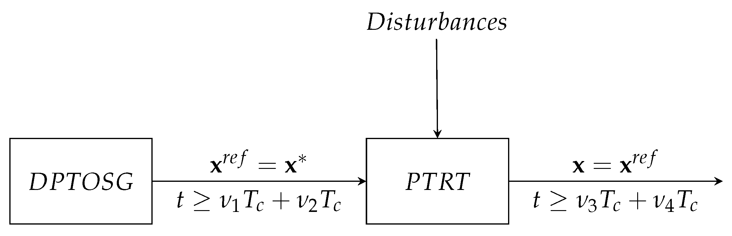
Abstract
:1. Introduction
- The algorithm can be applied to undirected graphs and detail-balanced graphs. None of the discussed papers considers this extension.
- The initial optimization step of the algorithm requires fewer adjustable parameters than many other algorithms found in the literature.
- Compared to many existing works, the gradients and Hessians are not shared among agents.
- Contrary to [25], the proposed algorithm is robust in the presence of matched disturbances and does not use a TBG.
2. Preliminaries
2.1. Notation
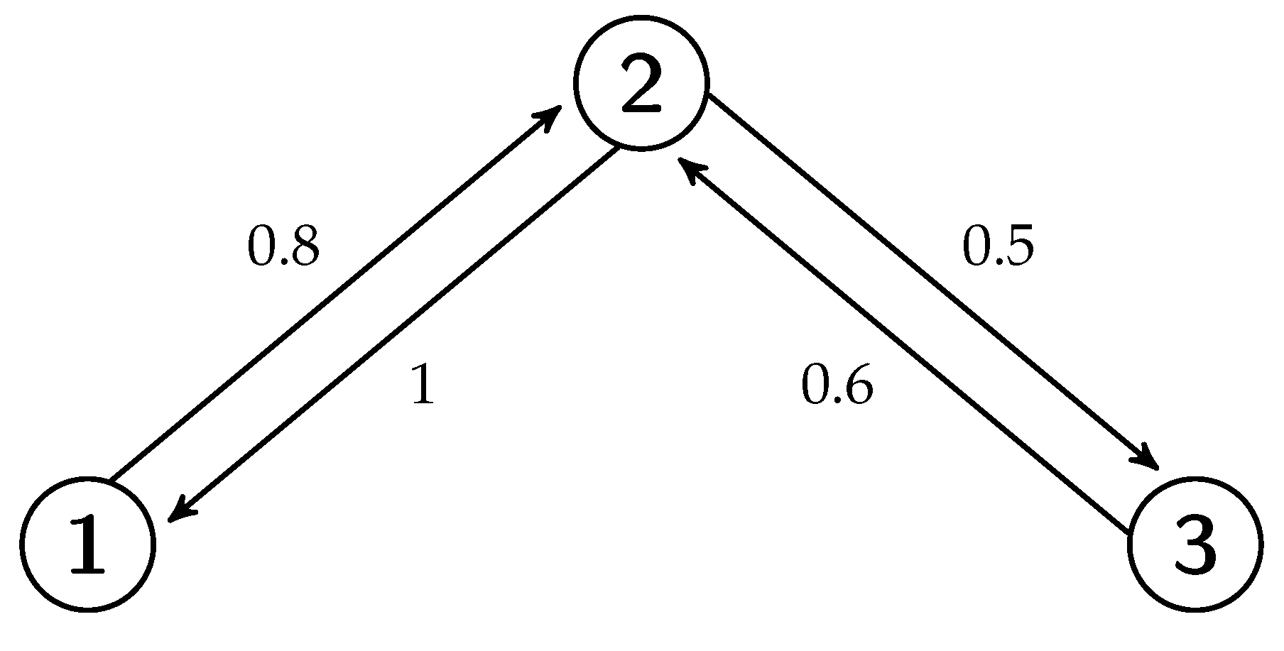
2.2. Graph Theory
2.3. Convex Analysis
2.4. Predefined-Time Stability
- Lyapunov is stable if for any , the solution is defined for all , and for any , there is such that for any , if then for all ;
- It is finite-time stable if it is Lyapunov stable and for any , there exists such that for all . The function is said the settling-time function of system (2);
- It is fixed-time stable if it is finite-time stable, and the settling-time function of system (2), , is bounded on , i.e., there exists such that ;
- It is predefined-time stable if it is fixed-time stable and for any there exists some such that the settling-time function of system (2) satisfies
3. Problem Statement
4. Main Results
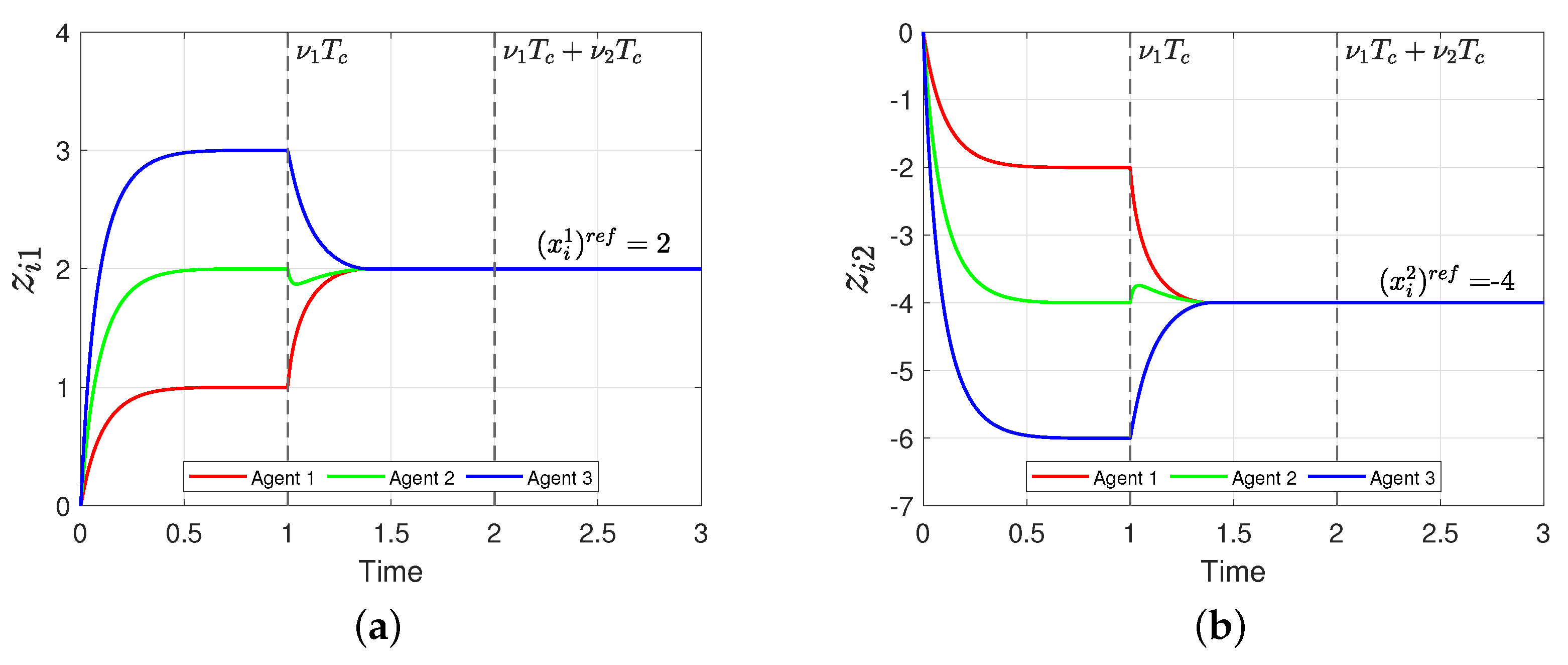
4.1. Distributed Predefined-Time Optimal Signal Generator (DPTOSG)
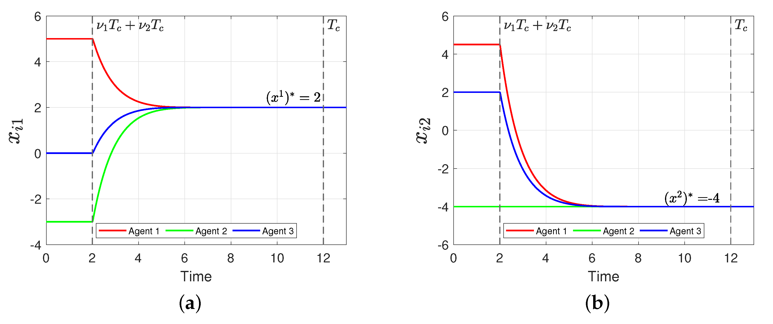
4.2. Predefined-Time Reference Tracking—PTRT
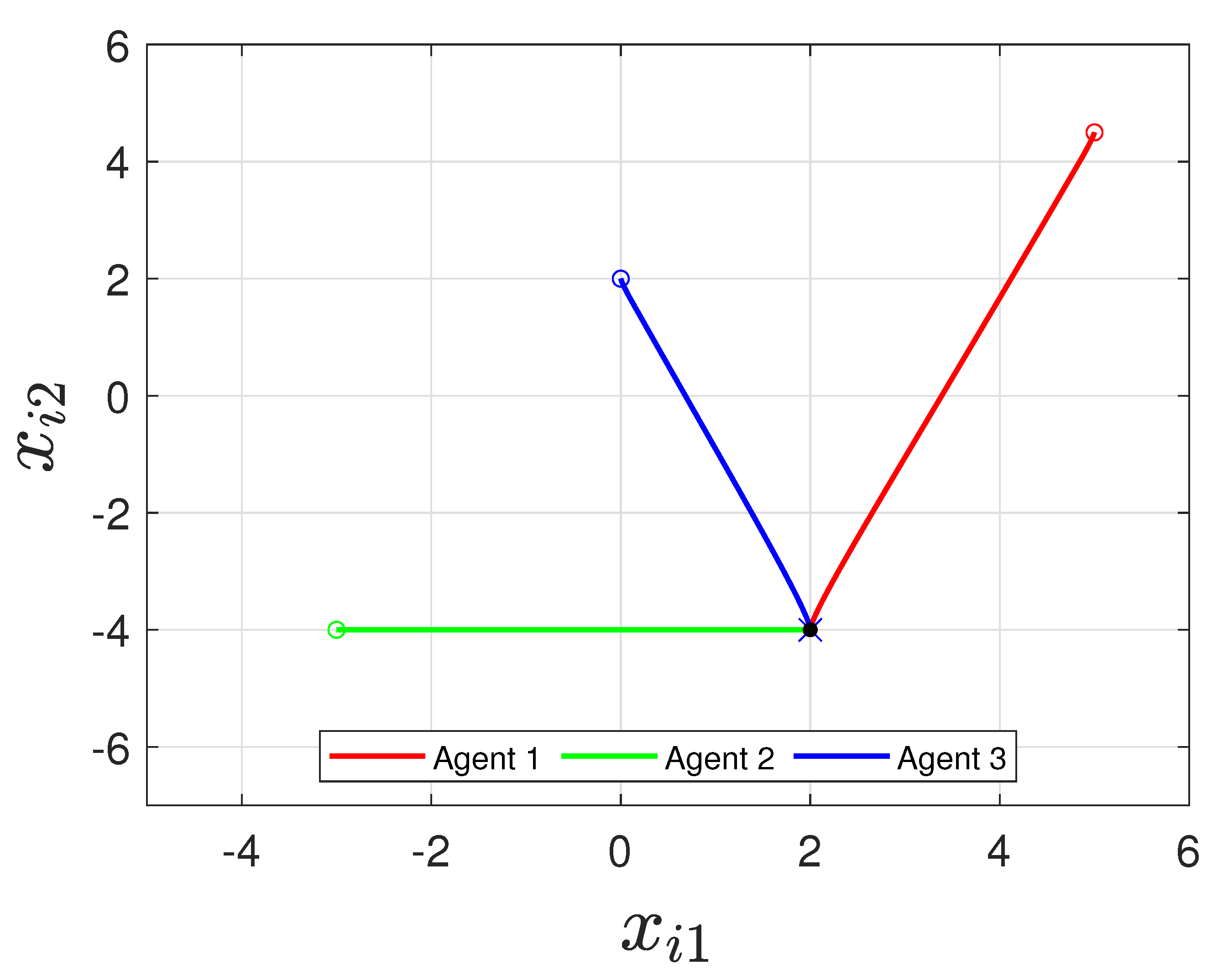
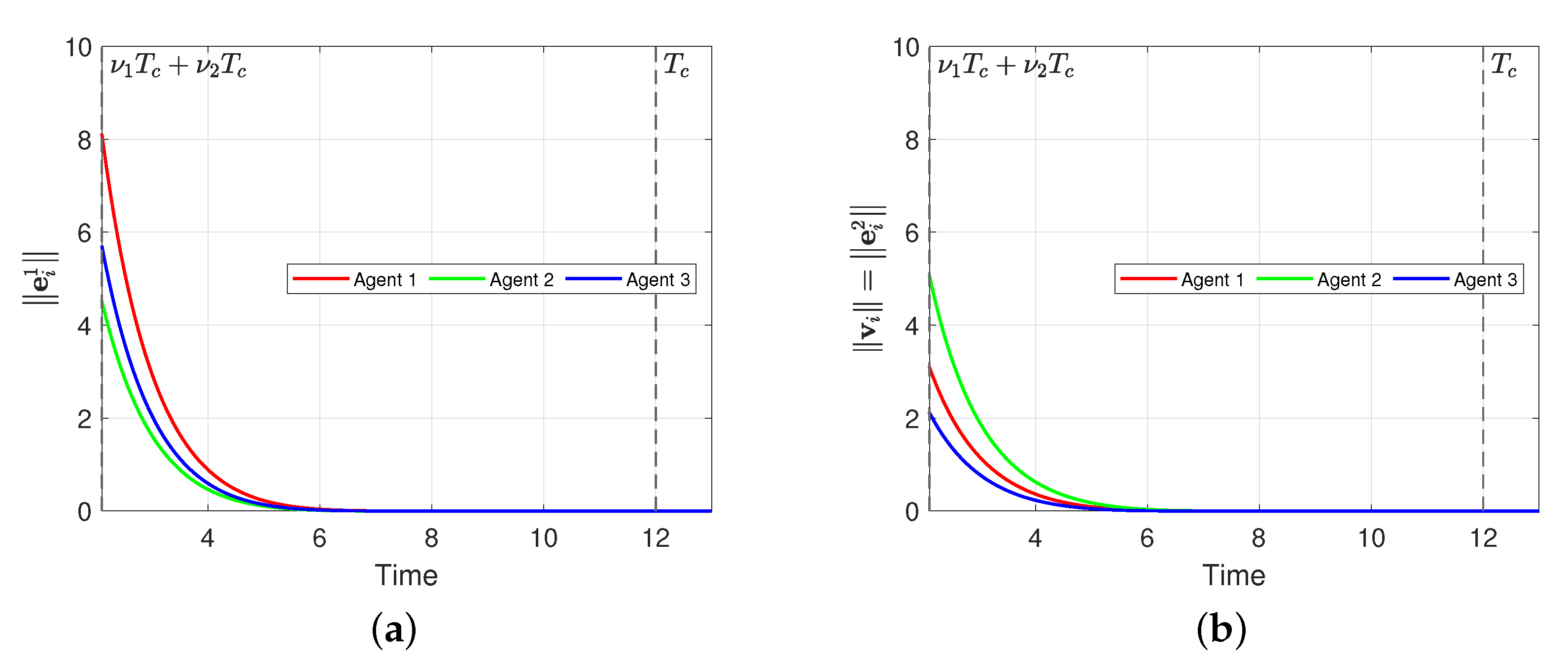
5. Numerical Example
6. Conclusions and Future Work
Author Contributions
Funding
Institutional Review Board Statement
Informed Consent Statement
Data Availability Statement
Conflicts of Interest
Abbreviations
| DPTOSG | Distributed Predefined-Time Optimal Signal Generator |
| MAS | Multi-Agent System |
| PTRT | Predefined-Time Reference Tracking |
| TBG | Time-Base Generator |
| UBST | Upper Bound of the Settling Time |
| ZGS | Zero Gradient Sum |
Appendix A. Useful lemmas
References
- Shi, X.; Cao, J.; Wen, G.; Perc, M. Finite-time consensus of opinion dynamics and its applications to distributed optimization over digraph. IEEE Trans. Cybern. 2018, 49, 3767–3779. [Google Scholar] [CrossRef] [PubMed]
- Dai, H.; Fang, X.; Jia, J. Consensus-based distributed fixed-time optimization for a class of resource allocation problems. J. Frankl. Inst. 2022, 359, 11135–11154. [Google Scholar] [CrossRef]
- Mao, S.; Tang, Y.; Dong, Z.; Meng, K.; Dong, Z.Y.; Qian, F. A privacy preserving distributed optimization algorithm for economic dispatch over time-varying directed networks. IEEE Trans. Ind. Inform. 2020, 17, 1689–1701. [Google Scholar] [CrossRef]
- Dougherty, S.; Guay, M. An extremum-seeking controller for distributed optimization over sensor networks. IEEE Trans. Autom. Control 2016, 62, 928–933. [Google Scholar] [CrossRef]
- Nedic, A. Distributed gradient methods for convex machine learning problems in networks: Distributed optimization. IEEE Signal Process. Mag. 2020, 37, 92–101. [Google Scholar] [CrossRef]
- Yang, T.; Yi, X.; Wu, J.; Yuan, Y.; Wu, D.; Meng, Z.; Hong, Y.; Wang, H.; Lin, Z.; Johansson, K.H. A survey of distributed optimization. Annu. Rev. Control 2019, 47, 278–305. [Google Scholar] [CrossRef]
- Zak, M. Terminal attractors in neural networks. Neural Netw. 1989, 2, 259–274. [Google Scholar] [CrossRef]
- Polyakov, A. Nonlinear Feedback Design for Fixed-Time Stabilization of Linear Control Systems. IEEE Trans. Autom. Control 2012, 57, 2106–2110. [Google Scholar] [CrossRef] [Green Version]
- Sánchez-Torres, J.D.; Gómez-Gutiérrez, D.; López, E.; Loukianov, A.G. A class of predefined-time stable dynamical systems. IMA J. Math. Control. Inf. 2018, 35, i1–i29. [Google Scholar] [CrossRef] [Green Version]
- Jiménez-Rodríguez, E.; Muñoz-Vázquez, A.J.; Sánchez-Torres, J.D.; Defoort, M.; Loukianov, A.G. A Lyapunov-like characterization of predefined-time stability. IEEE Trans. Autom. Control 2020, 65, 4922–4927. [Google Scholar] [CrossRef] [Green Version]
- Aldana-López, R.; Gómez-Gutiérrez, D.; Jiménez-Rodríguez, E.; Sánchez-Torres, J.D.; Defoort, M. Generating new classes of fixed-time stable systems with predefined upper bound for the settling time. Int. J. Control 2022, 95, 2802–2814. [Google Scholar] [CrossRef]
- Sánchez-Torres, J.D.; Defoort, M.; Muñoz-Vázquez, A.J. Predefined-time stabilisation of a class of nonholonomic systems. Int. J. Control 2020, 93, 2941–2948. [Google Scholar] [CrossRef]
- Aldana-López, R.; Gómez-Gutiérrez, D.; Jiménez-Rodríguez, E.; Sánchez-Torres, J.D.; Loukianov, A.G. On predefined-time consensus protocols for dynamic networks. J. Frankl. Inst. 2020, 357, 11880–11899. [Google Scholar] [CrossRef]
- Jiménez-Rodríguez, E.; Aldana-López, R.; Sánchez-Torres, J.D.; Gómez-Gutiérrez, D.; Loukianov, A.G. Consistent Discretization of a Class of Predefined-Time Stable Systems. In Proceedings of the 21st IFAC World Congress 2020—1st Virtual IFAC World Congress (IFAC-V 2020), Berlin, Germany, 11–17 July 2020. [Google Scholar]
- Ning, B.; Han, Q.L.; Zuo, Z. Distributed optimization of multiagent systems with preserved network connectivity. IEEE Trans. Cybern. 2018, 49, 3980–3990. [Google Scholar] [CrossRef] [PubMed]
- Chen, G.; Li, Z. A fixed-time convergent algorithm for distributed convex optimization in multi-agent systems. Automatica 2018, 95, 539–543. [Google Scholar] [CrossRef]
- Wang, X.; Wang, G.; Li, S. A distributed fixed-time optimization algorithm for multi-agent systems. Automatica 2020, 122, 109289. [Google Scholar] [CrossRef]
- Gong, X.; Cui, Y.; Shen, J.; Xiong, J.; Huang, T. Distributed Optimization in Prescribed-Time: Theory and Experiment. IEEE Trans. Netw. Sci. Eng. 2021, 9, 564–576. [Google Scholar] [CrossRef]
- Deng, Z.; Chen, T. Distributed algorithm design for constrained resource allocation problems with high-order multi-agent systems. Automatica 2022, 144, 110492. [Google Scholar] [CrossRef]
- Ma, L.; Hu, C.; Yu, J.; Wang, L.; Jiang, H. Distributed Fixed/Preassigned-Time Optimization Based on Piecewise Power-Law Design. IEEE Trans. Cybern. 2022. [Google Scholar] [CrossRef]
- Tang, Y. Distributed optimization for a class of high-order nonlinear multiagent systems with unknown dynamics. Int. J. Robust Nonlinear Control 2018, 28, 5545–5556. [Google Scholar] [CrossRef] [Green Version]
- Adibzadeh, A.; Suratgar, A.A.; Menhaj, M.B.; Zamani, M. Distributed optimization in heterogeneous dynamical networks. Iran. J. Sci. Technol. Trans. Electr. Eng. 2020, 44, 473–483. [Google Scholar] [CrossRef]
- Wang, X.; Wang, G.; Li, S. Distributed finite-time optimization for integrator chain multiagent systems with disturbances. IEEE Trans. Autom. Control 2020, 65, 5296–5311. [Google Scholar] [CrossRef]
- Tran, N.T.; Wang, Y.W.; Yang, W. Distributed optimization problem for double-integrator systems with the presence of the exogenous disturbance. Neurocomputing 2018, 272, 386–395. [Google Scholar] [CrossRef]
- Li, S.; Nian, X.; Deng, Z.; Chen, Z. Predefined-time distributed optimization of general linear multi-agent systems. Inf. Sci. 2022, 584, 111–125. [Google Scholar] [CrossRef]
- Aldana-López, R.; Seeber, R.; Haimovich, H.; Gómez-Gutiérrez, D. On inherent robustness and performance limitations of a class of prescribed-time algorithms. arXiv 2022, arXiv:2205.02528. [Google Scholar]
- Yu, Z.; Yu, S.; Jiang, H.; Mei, X. Distributed fixed-time optimization for multi-agent systems over a directed network. Nonlinear Dyn. 2021, 103, 775–789. [Google Scholar] [CrossRef]
- Boyd, S.; Boyd, S.P.; Vandenberghe, L. Convex Optimization; Cambridge University Press: Cambridge, UK, 2004. [Google Scholar]
- Hiriart-Urruty, J.B. Optimisation et Analyse Convexe: Exercices Corrigés; In the Series Enseignement SUP-Maths; EDP Sciences: Les Ulis, France, 2009. [Google Scholar]
- Lin, W.T.; Wang, Y.W.; Li, C.; Yu, X. Predefined-time optimization for distributed resource allocation. J. Frankl. Inst. 2020, 357, 11323–11348. [Google Scholar] [CrossRef]
- Lu, J.; Tang, C.Y. Zero-gradient-sum algorithms for distributed convex optimization: The continuous-time case. IEEE Trans. Autom. Control 2012, 57, 2348–2354. [Google Scholar] [CrossRef] [Green Version]
- Ren, W.; Beard, R.W. Distributed Consensus in Multi-Vehicle Cooperative Control; Springer: London, UK, 2008. [Google Scholar]


Disclaimer/Publisher’s Note: The statements, opinions and data contained in all publications are solely those of the individual author(s) and contributor(s) and not of MDPI and/or the editor(s). MDPI and/or the editor(s) disclaim responsibility for any injury to people or property resulting from any ideas, methods, instructions or products referred to in the content. |
© 2023 by the authors. Licensee MDPI, Basel, Switzerland. This article is an open access article distributed under the terms and conditions of the Creative Commons Attribution (CC BY) license (https://creativecommons.org/licenses/by/4.0/).
Share and Cite
De Villeros, P.; Sánchez-Torres, J.D.; Muñoz-Vázquez, A.J.; Defoort, M.; Fernández-Anaya, G.; Loukianov, A. Distributed Predefined-Time Optimization for Second-Order Systems under Detail-Balanced Graphs. Machines 2023, 11, 299. https://doi.org/10.3390/machines11020299
De Villeros P, Sánchez-Torres JD, Muñoz-Vázquez AJ, Defoort M, Fernández-Anaya G, Loukianov A. Distributed Predefined-Time Optimization for Second-Order Systems under Detail-Balanced Graphs. Machines. 2023; 11(2):299. https://doi.org/10.3390/machines11020299
Chicago/Turabian StyleDe Villeros, Pablo, Juan Diego Sánchez-Torres, Aldo Jonathan Muñoz-Vázquez, Michael Defoort, Guillermo Fernández-Anaya, and Alexander Loukianov. 2023. "Distributed Predefined-Time Optimization for Second-Order Systems under Detail-Balanced Graphs" Machines 11, no. 2: 299. https://doi.org/10.3390/machines11020299