Article

Quasi-Coordinates-Based Closed-Form Dynamic Modeling and Analysis for a 2R1T PKM with a Rigid–Flexible Structure

1
Ningbo Institute of Materials Technology and Engineering, Chinese Academy of Sciences, Ningbo 315201, China
2
College of Materials Sciences and Opto-Electronic Technology, University of Chinese Academy of Sciences, Beijing 100049, China
3
Zhejiang Key Laboratory of Robotics and Intelligent Manufacturing Equipment Technology, Ningbo 315201, China
*
Author to whom correspondence should be addressed.
Machines 2023, 11(2), 260; https://doi.org/10.3390/machines11020260
Submission received: 27 December 2022 / Revised: 27 January 2023 / Accepted: 6 February 2023 / Published: 9 February 2023
(This article belongs to the Special Issue Dynamic Analysis of Multibody Mechanical Systems)

Abstract

:
This work derives a closed-form dynamic model for a two rotational and one translational degrees-of-freedom (2R1T) parallel kinematic mechanism (PKM) with a hybrid rigid–flexible structure for force-control applications. Based on the three-prismatic-prismatic-spherical (3PPS) kinematic configuration of the 2R1T PKM and its zero-torsion motion characteristics, a symbolic formulation approach is proposed to establish closed-form kinematic models for both forward and inverse kinematics analysis. As the moving platform pose of the 2R1T 3PPS PKM can be readily determined by the three active prismatic joint variables and the three passive prismatic joint variables, these six joint variables are selected as the quasi-coordinates so as to systematically develop the closed-form dynamic model with a Lagrangian formulation, in which the stiffness and deformation of the three flexure-based passive prismatic joints are uniformly taken into consideration. Through eliminating the three passive prismatic joint variables based on the principle of virtual work and the relationships between the active and passive prismatic joint variables, a closed-form dynamic model for the 2R1T 3PPS PKM with a rigid–flexible structure is finally obtained. The correctness of the closed-form dynamic model was validated with the commercial dynamic simulation software. Utilizing the closed-form dynamic model, the effects of different flexure stiffness in driving directions on the required active joint force were investigated, which indicated that little flexure stiffness in driving directions is desired.

1. Introduction

A parallel kinematic mechanism (PKM) offers the advantages of high stiffness, high payload capacity, high precision, and low moving mass at the expense of a small workspace and a complex mechanical structure. Among various PKMs, the 3DOF 2R1T PKMs are one class of lower-mobility PKMs which have drawn increasing attention due to their simpler mechanical structures and lower fabrication costs compared with 6DOF PKMs [1,2,3]. The 3DOF 2R1T PKMs have been employed in many industrial applications, e.g., in a tool head [4], a rehabilitation device [5], and a force-controlled end-effector [6]. Dynamic modeling of such PKMs is essential and important for their design optimization and development of model-based control algorithms.
To formulate the equations of motion of conventional rigid PKMs, two fundamental approaches have been established, namely, the vectorial mechanics approach and the analytical mechanics approach. The former is based on the Newton–Euler laws for deriving equations of motion using Cartesian coordinates and kinematic constraints [7,8], and the latter is based on the Lagrangian formulation involving kinetic energy and potential energy [9,10,11]. In addition, Kane’s method [12,13] and the principle of virtual work [14,15,16] are also widely-used methods. The Newton–Euler formulation requires the computations of all the internal constraint forces and moments between adjacent joints. The modeling procedure is straightforward but leads to a large number of recursive equations. As such, the Newton–Euler formulation is not an attractive choice for model-based control of PKMs. The Lagrangian formulation offers the advantages of deriving the closed-form dynamic models for serial manipulators. However, for multi-closed-chain PKMs, it involves with rather complex mathematical manipulations to deal with the unknown passive joint variables which are dependent on the active joint variables. Kane’s method employs Lagrange’s form of the d’Alembert principle and can automatically eliminate “no-working” internal constraint forces, and the concept of partial velocity was introduced for it.
The principle of virtual work is an energy-based formulation with a relatively simple symbolic description that allows elimination of all reaction forces and moments. Similarly to the Lagrangian formulation, both Kane’s method and the principle of the virtual work method encounter difficulties in formulating the closed-form dynamic models for PKMs.
With respect to the dynamic formulation of flexible PKMs, the analytical approach for complex flexible PKMs is almost impossible. Many discretization strategies, including the lumped parameter method [17], assumed mode method [18], finite element method [19], and finite segment method [20], have been investigated to transform a full-order system to a reduced-order system. There are trade-offs between accuracy and efficiency among these methods. The studies about the dynamic performance of fully flexure-based PKMs mainly focus on the resonance frequencies and harmonic response [21,22]. The majority of publications referring to the flexible PKM dynamics mainly focus on the link flexibility [23,24,25], e.g., the PKMs designed with lightweight and slim links to achieve high-speed motion in pick-and-place applications [26]. The movable links are modeled by beam elements or finite segments, so that the coupling effects of rigid motions and flexible motions can be analyzed by kineto-elasto dynamics and flexible multibody dynamics [27]. Still, the dynamics of PKM with flexure-based joints are less addressed, and the conventional kinematic and dynamic analysis methods encounter difficulties with obtaining the closed-form kinematic and dynamic models for a PKM with a rigid–flexible structure. Moreover, the coupling effects of flexure-based joints on the system dynamic behavior have not been investigated thoroughly. The systematic investigation of dynamic modeling and analysis of the PKM with a rigid–flexible structure is still an open problem.
Among the previous studies related to the 2R1T 3-legged prismatic-prismatic-spherical (3PPS) PKMs with flexure-based joints, a flexure-based 2R1T 3PPS PKM for nano-positioning applications was proposed in [28,29], and a 2R1T 3PPS PKM with a rigid–flexible structure was proposed as a force-controlled robot end-effector, in which the three flexure-based passive prismatic joints are employed [30,31]. However, the dynamic modeling on such PKM rigid–flexible configurations has not been carried out. We developed a simplified systematic modeling method to formulate the closed-form dynamic model for the 2R1T 3PPS PKM with a rigid–flexible structure. Based on the zero-torsion motion characteristic of the 2R1T 3PPS PKM, the homogeneous transformation matrix describing the moving platform pose can be described with linear polynomials of both active and passive prismatic joint variables. The closed-form model for both forward and inverse kinematic analysis was then obtained. To simplify the dynamic modeling procedure, these six prismatic joint variables were selected as the quasi-coordinates for Lagrangian formulation. By virtue of the quasi-coordinates, the kinetic energy and potential energy of the 2R1T 3PPS PKM can be readily obtained, which makes the overall derivation of closed-form dynamic model in terms of the six quasi-coordinates significantly simplified. Then, three passive prismatic joint variables were eliminated based on the principle of virtual work and the relationships between the active and passive prismatic joint variables. As such, a closed-form dynamic model for the 2R1T 3PPS PKM with a rigid–flexible structure in terms of the three active prismatic joint variables was obtained. The correctness of the derived closed-form dynamic model was validated with the commercial dynamic simulation software. The coupling effects of the flexure-based passive prismatic joints on the required active joint forces were investigated and are discussed.
The rest of this paper is organized as follows. In Section 2, the closed-form kinematic model of the 2R1T 3PPS PKM is briefly revisited. In Section 3, the quasi-coordinates are introduced. Then, a closed-form dynamics modeling approach using the Lagrangian formulation and the principle of virtual work is proposed and validated. In Section 4, the effects of the flexure-based passive prismatic joints on the required active joint forces are presented based on the derived closed-form dynamic model. In Section 5, the results presented in Section 3 and Section 4 are discussed. Finally, Section 6 summarizes this paper.

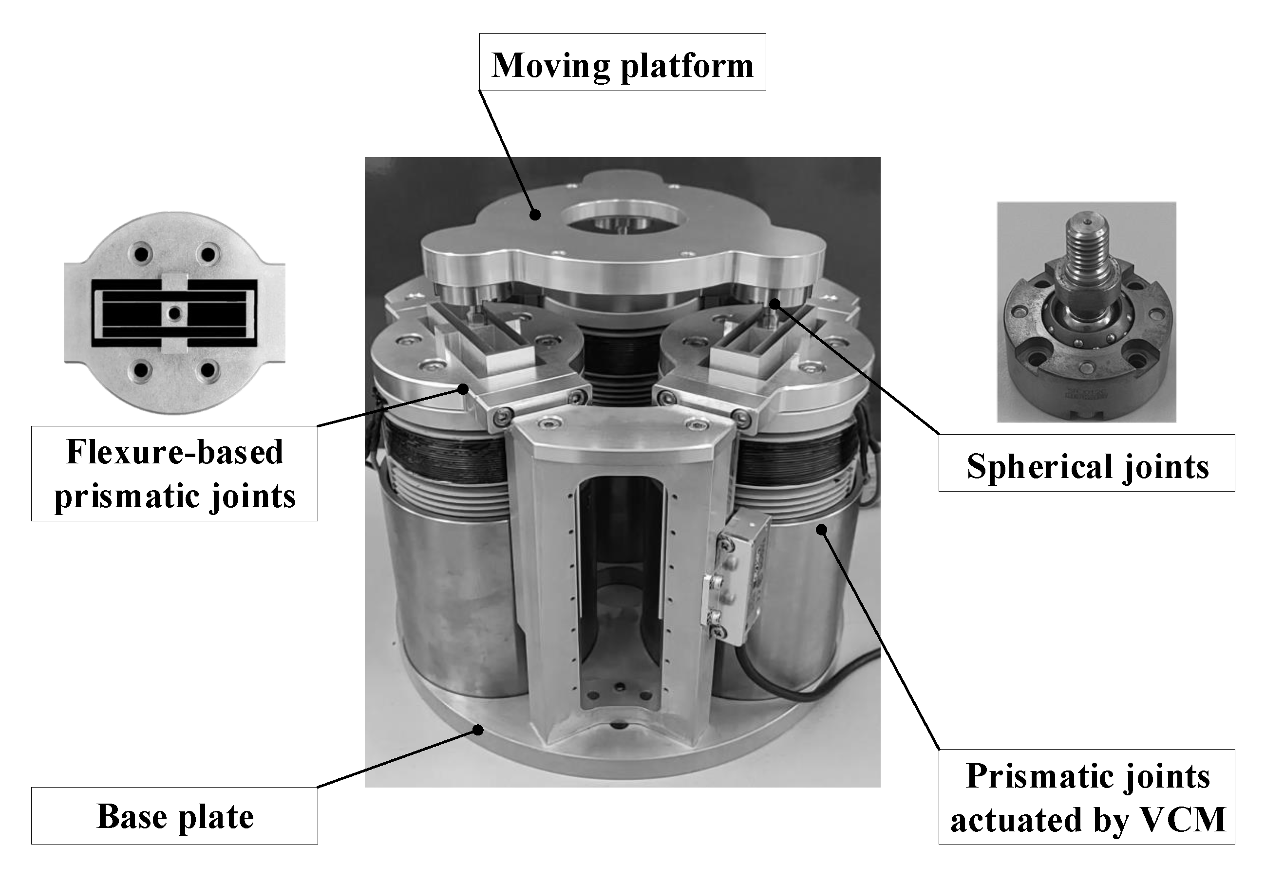
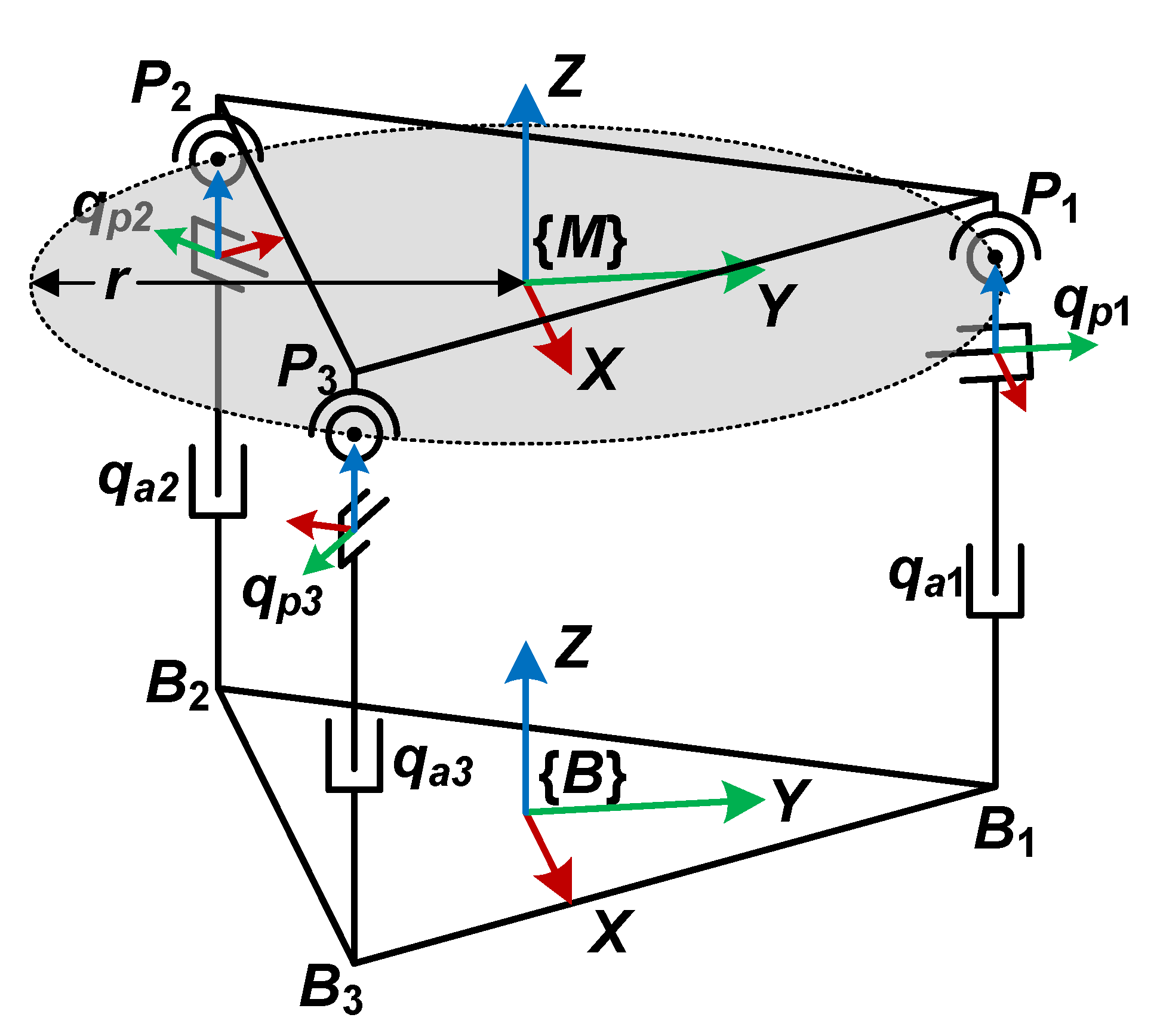
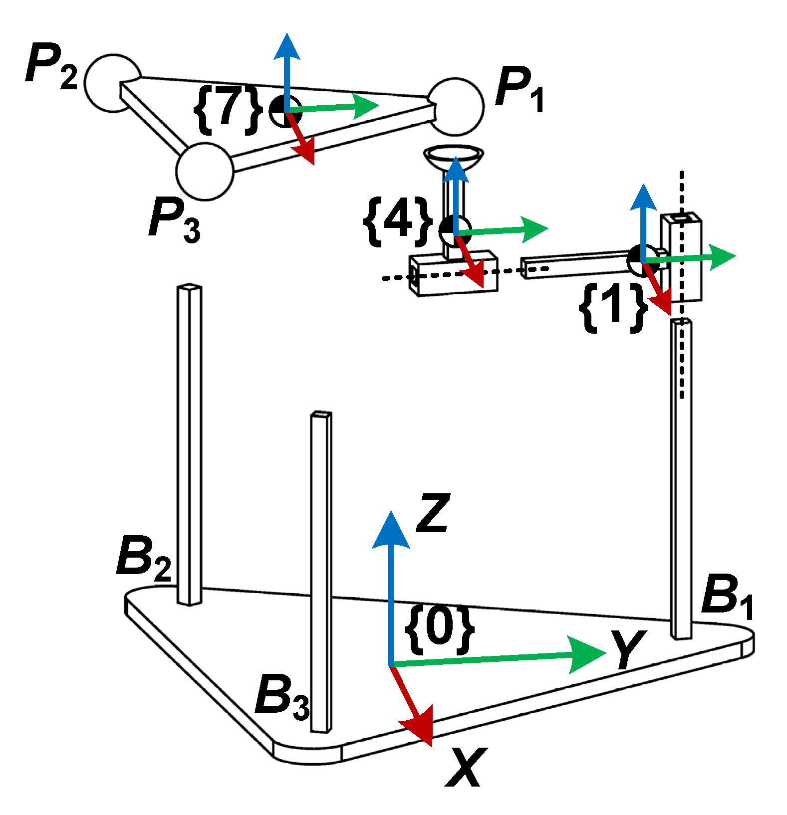
2. Kinematic Modeling of the 2R1T 3PPS PKM

The proposed 2R1T PKM has a 3PPS (P stands for prismatic joint and S stands for spherical joint) configuration, which is employed as a robotic force-controlled end-effector for continuous contact operations, as shown in Figure 1. It has a symmetric structure with three identical PPS legs placed 120 apart. Each leg consists of a vertical active prismatic joint driven by a voice coil motor (VCM), a horizontal flexure-based passive prismatic joint with high off-axis stiffness ratio, and a passive spherical joint [30].

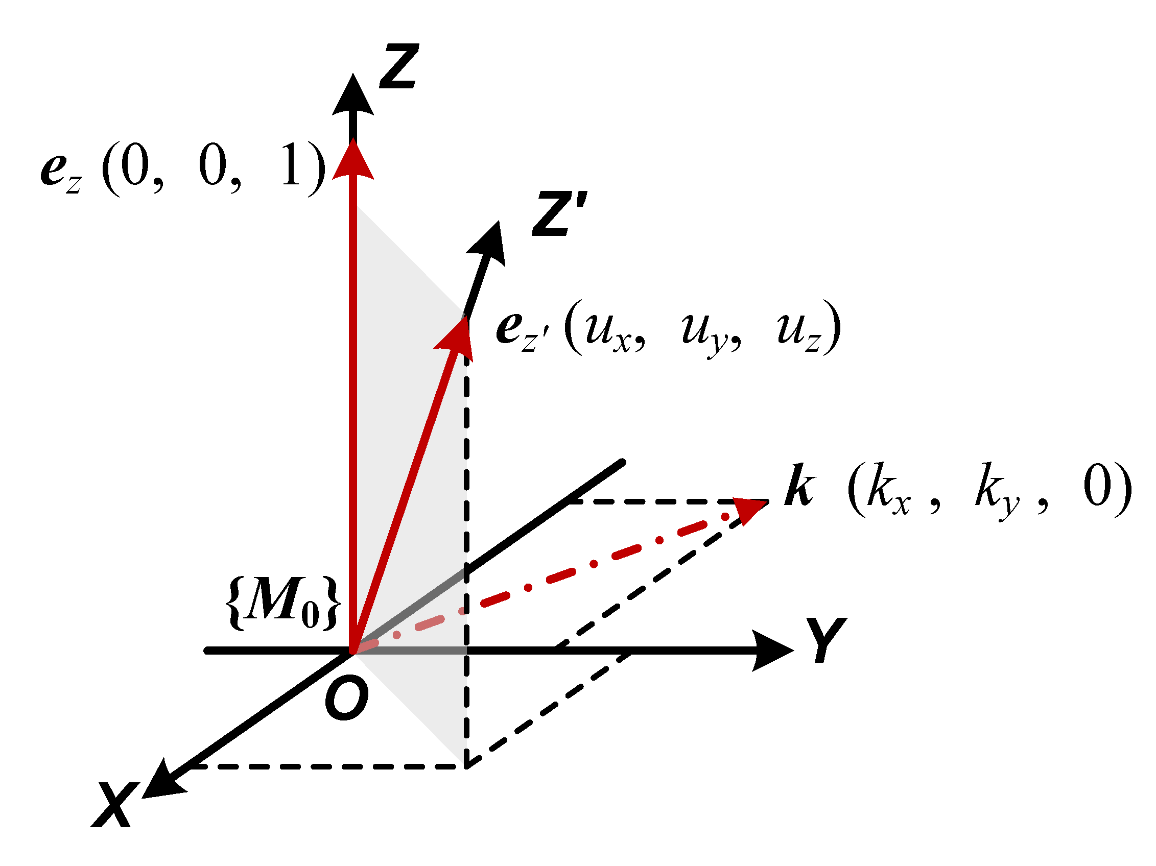
2.1. Displacement Modeling

The kinematic diagram of the 2R1T 3PPS PKM is shown in Figure 2. The base frame B is attached to the center of the base plate with its z axis perpendicular to the base plate and the x axis parallel to B 2 B 3 . The moving platform frame M is attached to the center of Δ P 1 P 2 P 3 , its z axis is perpendicular to Δ P 1 P 2 P 3 , and the x axis is parallel to P 2 P 3 . The positive direction of each active prismatic joint displacement is along the + z direction of the base frame, and the positive direction of each passive prismatic joint displacement is along the + y direction of its body frame.
For the zero-torsion 3PPS parallel mechanism, our previous work [30] proposed two parameters ( u x , u y ) to describe the orientation of the moving platform, as shown in Figure 3. Parameters u x and u y represent the x and y coordinates of the unit z axis vector of the moving platform with respect to frame M 0 , respectively. It is noted that frame M 0 is attached to the origin of moving platform frame M with the same orientation as the base frame B. The proposed orientation description is intuitive, as the orientation of the moving platform is equivalent to rotation about a unit axis k parallel to the base plate.
Based on the zero-torsion motion characteristic of the 3PPS PKM, the rotation matrix is simplified as follows:
R M B = R 11 R 21 R 31 R 21 R 22 R 32 R 31 R 32 R 11 + R 22 1
where R i j denotes the entry in the ith row and jth column of the rotation matrix.
Based on the structure characteristics and joint configurations of the 3PPS PKM, the homogeneous transformation matrix can also be derived in terms of active and passive prismatic joint coordinates.
R M B = q p 2 + q p 3 + 2 r 2 r q p 2 q p 3 2 3 r q p 3 q a 2 q a 1 + q p 2 q a 1 q a 3 + q a 2 q a 3 2 q p 1 + 3 r 3 3 r 2 q p 2 q p 3 2 3 r 4 q p 1 + q p 2 + q p 3 + 6 r 6 r q a 1 q p 2 q p 3 2 r + q a 2 q p 3 + r + q a 3 q p 2 + r 3 r 2 q a 3 q a 2 3 r 2 q a 1 q a 2 q a 3 3 r q p 1 q p 2 + q p 3 + 2 r + q p 2 q p 3 + 2 r + r 2 q p 3 + 3 r 3 r 2
P M B = q p 3 q p 2 2 3 2 q p 1 q p 2 q p 3 6 3 H B M + q a 1 + q a 2 + q a 3 3
where q a i and q p i denote the active and passive prismatic joint coordinates of the ith leg, respectively.
From Equations (1)–(3) can be further simplified as
R M B = q p 2 + q p 3 + 2 r 2 r q p 2 q p 3 2 3 r q a 3 + q a 2 3 r q p 2 q p 3 2 3 r 4 q p 1 + q p 2 + q p 3 + 6 r 6 r 2 q a 1 + q a 2 + q a 3 3 r q a 3 q a 2 3 r 2 q a 1 q a 2 q a 3 3 r 2 q p 1 + q p 2 + q p 3 + 3 r 3 r
P M B = r · R 21 r R 22 R 11 2 M z
According to the Rodrigues formula and the two-parameter orientation description ( u x , u y ), such a rotation in Equation (4) can be determined as
R M B = u x 2 u z + u y 2 u x 2 + u y 2 u x u y u z 1 u x 2 + u y 2 u x u x u y u z 1 u x 2 + u y 2 u x 2 + u y 2 u z u x 2 + u y 2 u y u x u y u z
where u z = 1 u x 2 u y 2 .
According to Equations (3)–(6), the closed-form forward displacement solution is derived as [30]
u x = q a 2 q a 3 3 r
u y = 2 q a 1 + q a 2 + q a 3 3 r
M z = H B M + q a 1 + q a 2 + q a 3 3
where M z is the z-coordinate of the origin of the moving platform frame M with respect to the base frame B, q a i is the active joint variables in the ith leg, r is the radius of the circumcircle passing through three centers of the sphere joints, and H B M is the distance between the origins of frames B and M when all three active joints are at the minimal strokes, i.e., home positions.
Based on Equations (4)–(9), the homogeneous transformation matrix can be described with linear polynomials of both active and passive prismatic joint variables.
The inverse displacement solution is derived readily from the closed-form forward displacement solution, i.e., Equations (7)–(9), as follows:
q a 1 = M z H B M r · u y
q a 2 = M z H B M + r 2 3 u x + u y
q a 3 = M z H B M + r 2 3 u x + u y

2.2. Velocity and Acceleration Analysis

The Cartesian velocity vectors of the moving platform and active joint velocities are related as follows:
q ˙ a = J 1 V M = q ˙ a 1 q ˙ a 2 q ˙ a 3 = J 1 ω x ω y v z
where V M 3 × 1 is the Cartesian velocity vector of the moving platform, and J is the kinematic Jacobian matrix of the PKM.
Differentiating Equation (13) with respect to time yields the acceleration mapping relationships:
q ¨ a = J 1 V ˙ M + J ˙ 1 V M

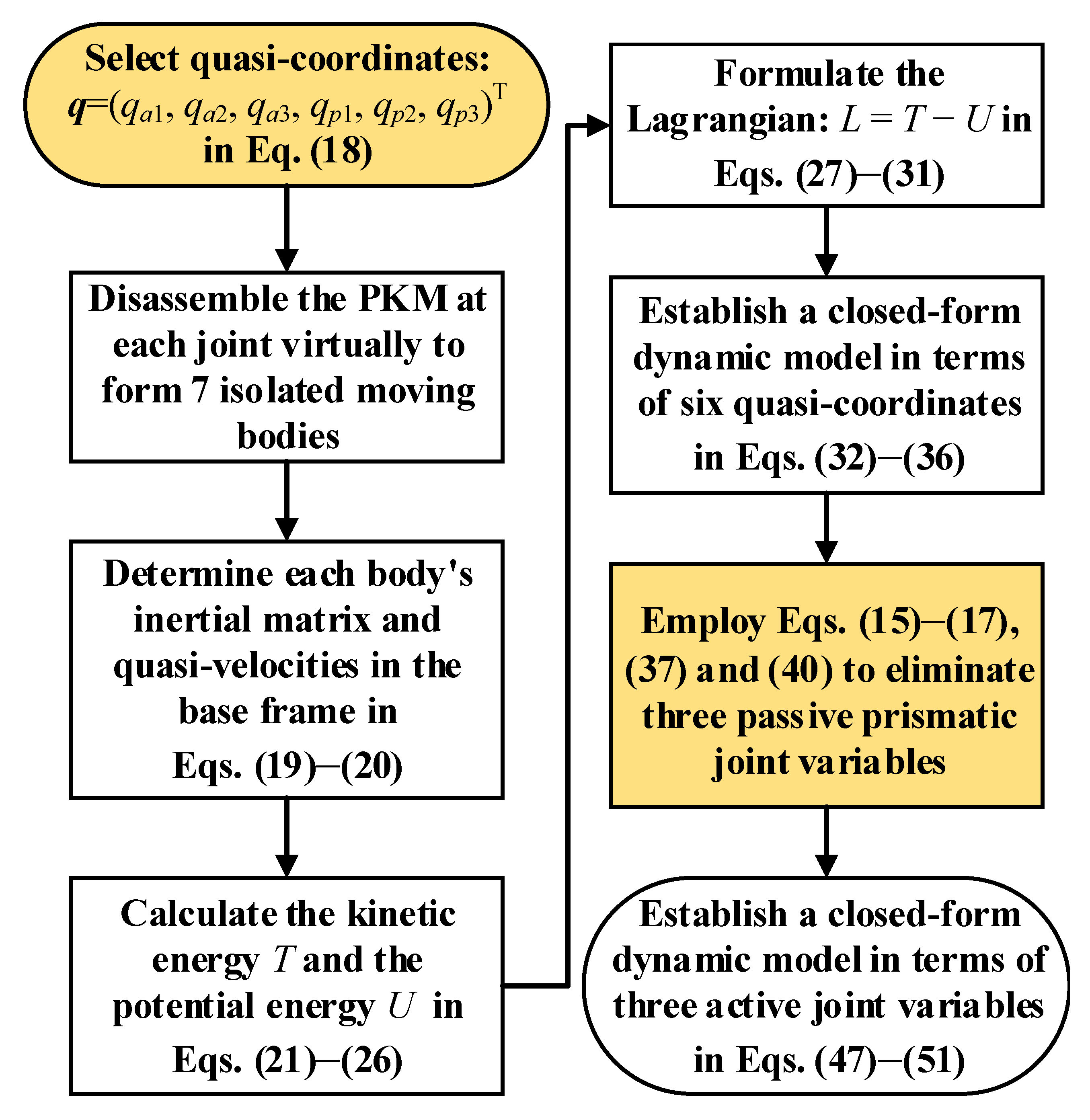
3. Dynamic Modeling of the 2R1T 3PPS PKM with a Rigid–Flexible Structure

For a general PKM, dynamic modeling with Lagrangian formulation is considered to be a nontrivial task due to the closed-chain structures of the system. In such a derivation, the number of independent generalized coordinates is equal to that of degrees of freedom. As such, in order to obtain the Lagrange’s equations of motion, a significant amount of mathematical manipulation is required to describe complex and nonlinear relations in terms of independent generalized coordinates. When it comes to the rigid and flexible multi-body dynamics, finite element analysis (FEA) is usually involved, with which is time-consuming to achieve enough accuracy and unlikely to be possible perform real-time dynamics computations in the controller. As for a given PKM, the symbolic closed-form equations are likely to be the most efficient formulations of dynamics [32].
In this section, a closed-form dynamic model of the 2R1T 3PPS PKM with a rigid–flexible structure is developed, which can be utilized as the basis of robot design, trajectory planning, and model-based control algorithms. The formulation procedure of the proposed dynamic modeling approach is presented, in which the quasi-coordinates are introduced and the stiffness in driving direction of three flexure-based passive prismatic joints is taken into consideration. A virtual prototype is developed, and the correctness of the closed-form dynamic model is validated with the results of commercial dynamic simulation software.

3.1. Closed-Form Dynamic Model

The Lagrangian formulation allows the equations of motion to be obtained based on scalar quantities, namely, kinetic energy and potential energy.
Based on the kinematic model in Section 2, the constraints between q a and q p can be simplified as
q p 1 = 0.5 r R 11 + 3 R 22 2
q p 2 = r R 11 + 3 R 12 1
q p 3 = r R 11 3 R 12 1
For this specific 2R1T 3PPS PKM, the constraints are functions of active joint coordinates which show high non-linearity and introduce complex mathematical manipulations in the dynamic modeling. Rather than directly deriving the closed-form dynamics in terms of the generalized coordinates (three active prismatic joint variables), a closed-form dynamics modeling approach based on the Lagrangian formulation and the principle of virtual work is proposed, as shown in Figure 4. There are eight steps to obtaining the closed-form dynamic model for the 2R1T 3PPS PKM with a rigid–flexible structure in terms of three active prismatic joint variables. Firstly, both active and passive prismatic joint variables are selected as the quasi-coordinates. The closed-chain kinematic structures of the 2R1T 3PPS PKM are disassembled virtually at each joint, and seven isolated moving bodies are obtained. The overall kinetic energy and potential energy are calculated, for which the stiffness in driving direction of three flexure-based passive prismatic joints is taken into consideration. Based on the Lagrangian formulation, the closed-form dynamics in terms of the quasi-coordinates is established. Then, the principle of virtual work and the relationships between the active and passive prismatic joint variables are employed to eliminate the dependent coordinates (three passive prismatic joint variables). Finally, the closed-form dynamic model for the 2R1T 3PPS PKM with a rigid–flexible structure in terms of the three active prismatic joint variables is established.
As shown in Figure 5, body frames fixed at center of mass (COM) of the three active prismatic joints are numbered from 1 to 3, body frames fixed at COM of the three passive prismatic joints are numbered from 4 to 6, body frame 7 is fixed at the COM of the moving platform with the same orientation as the frame M, and the fixed base frame B of the 2R1T 3PPS PKM is labeled as frame 0.
The quasi-coordinates q 6 × 1 are represented by
q = q a 1 q a 2 q a 3 q p 1 q p 2 q p 3 = q 1 q 2 q 3 q 4 q 5 q 6
The kinetic energy and potential energy of each body are expressed in the base frame. The inertia tensor I i com of the ith body expressed in its body frame is constant and independent of motion. The corresponding inertia tensor I i of the ith body is transformed to the base frame through a transformation defined as follows:
I i = R i 0 I i com R 0 i = I i x x I i x y I i x z I i y z I i y y I i y z I i z x I i z y I i z z
After the quasi-coordinates are introduced, the angular and linear velocities of the ith body can be described as
V i = ω i v i 6 × 1 = J V i q ˙
where J V i 6 × 6 is the Jacobian matrix mapping the quasi-velocity to the Cartesian velocity. Since the motion axes of the active and passive prismatic joint on each leg of the 2R1T 3PPS PKM are perpendicular to each other, the Jacobian matrices J V i ( i = 1 , 2 , . . . , 6 ) are all constant matrices which can simplify the derivation process.
The kinetic energy of body i is derived as
T i = 1 2 ω i I i ω i + 1 2 m i v i v i
The overall kinetic energy of the 3PPS PKM equals
T = 1 2 i = 1 7 ω i I i ω i + m i v i v i = 1 2 i = 1 7 q ˙ D i q ˙
D i = J V i M i J V i
The inertia matrix M i of the ith body is a 6 × 6 configuration-dependent matrix.
M i q = I i 0 3 × 3 0 3 × 3 m i E 3 × 3
The gravitational potential energy of the 3PPS PKM with respect to q is given by
U g = i = 1 7 m i g r i
As the flexure-based passive prismatic joints have high off-axis stiffness ratios, only the stiffness in driving directions of the flexure-based passive prismatic joints is considered in the rigid–flexible integrated dynamics. The elastic potential energy of the three flexure-based passive prismatic joints (bodies 4, 5, and 6) with respect to q is
U s = i = 4 6 1 2 k s i q i 2
The Lagrangian of the 3PPS PKM is defined as
L = T U
where the kinetic energy is denoted as T and the potential energy is denoted as U = U g + U s .
The Lagrange equation of motion is derived as
d d t L q ˙ k L q k = τ k , k = 1 , 2 , , 6
where τ k is the kth term of quasi-generalized force vector.
The partial derivatives of the Lagrangian with respect to the kth joint velocity are given by
L q ˙ k = i = 1 7 q ˙ q ˙ k D i q ˙ = i = 1 7 q ˙ q ˙ k J V i M i J V i q ˙
The first term on the left side of Equation (29) is derived as
d d t L q ˙ k = i = 1 7 q ˙ q ˙ k D ˙ i q ˙ + q ˙ q ˙ k D i q ¨
The second term on the left side of Equation (29) is derived as
L q k = 1 2 i = 1 7 q ˙ D i q k q ˙ i = 1 7 m i g r i q k U s q k
The Lagrangian formulation to derive the dynamics of isolated bodies with respect to the quasi-coordinates yields
M q q ¨ + C q , q ˙ q ˙ + N q = τ
where M is the inertia matrix, C is the coefficient matrix of the centrifugal force and Coriolis force, N is the gravity and stiffness-related term, and τ is the quasi-generalized force with respect to the quasi-coordinates.
M q = m 1 + m 4 m 2 + m 5 m 3 + m 6 m 4 m 5 m 6 E 6 × 6 + D 7 q 6 × 6
C q , q ˙ = D ˙ 7 q 1 2 q ˙ D 7 q 1 q ˙ D 7 q 2 q ˙ D 7 q 3 q ˙ D 7 q 4 q ˙ D 7 q 5 q ˙ D 7 q 6 6 × 6
N q = N G q + N K q = m 1 + m 4 g z + m 7 g z r 7 q 1 m 2 + m 5 g z + m 7 g z r 7 q 2 m 3 + m 6 g z + m 7 g z r 7 q 3 m 7 g z r 7 q 4 + k s 4 q 4 m 7 g z r 7 q 5 + k s 5 q 5 m 7 g z r 7 q 6 + k s 6 q 6 6 × 1
N K q = 0 0 0 k s 4 q 4 k s 5 q 5 k s 6 q 6 6 × 1
In order to obtain the closed-form dynamic model of the 2R1T 3PPS PKM with respect to the active prismatic joint variables, the items related to the passive prismatic joint variables need to be described with the active prismatic joint variables. The relationship between the quasi-velocity and the active joint velocity is given by
q ˙ = J q a q ˙ a
J q a = E 3 × 3 J q a 2 p 6 × 3
The Jacobian matrix relating the active and passive joint variables is given by
J q a 2 p = q 4 q 1 q 4 q 2 q 4 q 3 q 5 q 1 q 5 q 2 q 5 q 3 q 6 q 1 q 6 q 2 q 6 q 3
Differentiating Equation (37) with respect to time yields
q ¨ = J ˙ q a q ˙ a + J q a q ¨ a
J ˙ q a = 0 3 × 3 J ˙ q a 2 p 6 × 3
J ˙ q a 2 p = q ˙ a H 1 q ˙ a H 2 q ˙ a H 3 3 × 3
where H i n × n is the Hessian matrix with respect to the active joint variables
H i = 2 q 3 + i q 1 2 2 q 3 + i q 2 q 1 2 q 3 + i q 3 q 1 2 q 3 + i q 1 q 2 2 q 3 + i q 2 2 2 q 3 + i q 3 q 2 2 q 3 + i q 1 q 3 2 q 3 + i q 2 q 3 2 q 3 + i q 3 2 , i = 1 , 2 , 3
According to the principle of virtual work, the power generated by all constraint forces and torques is zero.
τ δ q = τ a δ q a
δ q = J q a δ q a
τ a = J q a τ
By substituting Equations (37)–(46) into Equation (32), the closed-form dynamics with respect to the active joint variables is obtained
M ˜ q a q ¨ a + C ˜ q a , q ˙ a q ˙ a + N ˜ q a = τ a
where M ˜ is the inertia matrix, C ˜ is the coefficient matrix of the centrifugal force and Coriolis force, and N ˜ are the gravity and stiffness-related forces.
M ˜ q a = J q a M q J q a
C ˜ q a , q ˙ a = J q a M q J ˙ q a + J q a C q , q ˙ J q a
N ˜ q a = J q a N q
N ˜ K q a = J q a N K q = J q a 2 p k s 4 q 4 k s 5 q 5 k s 6 q 6

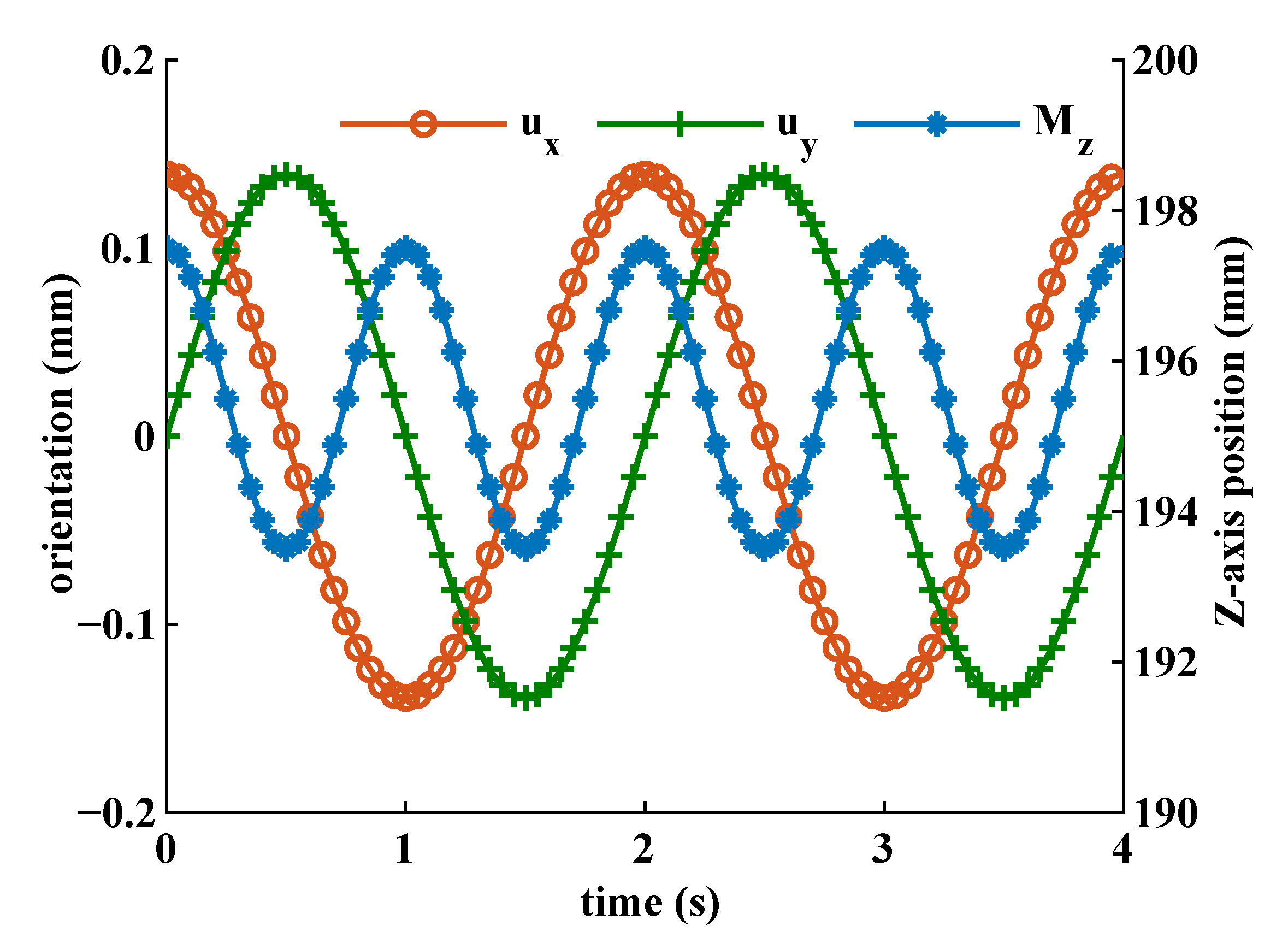
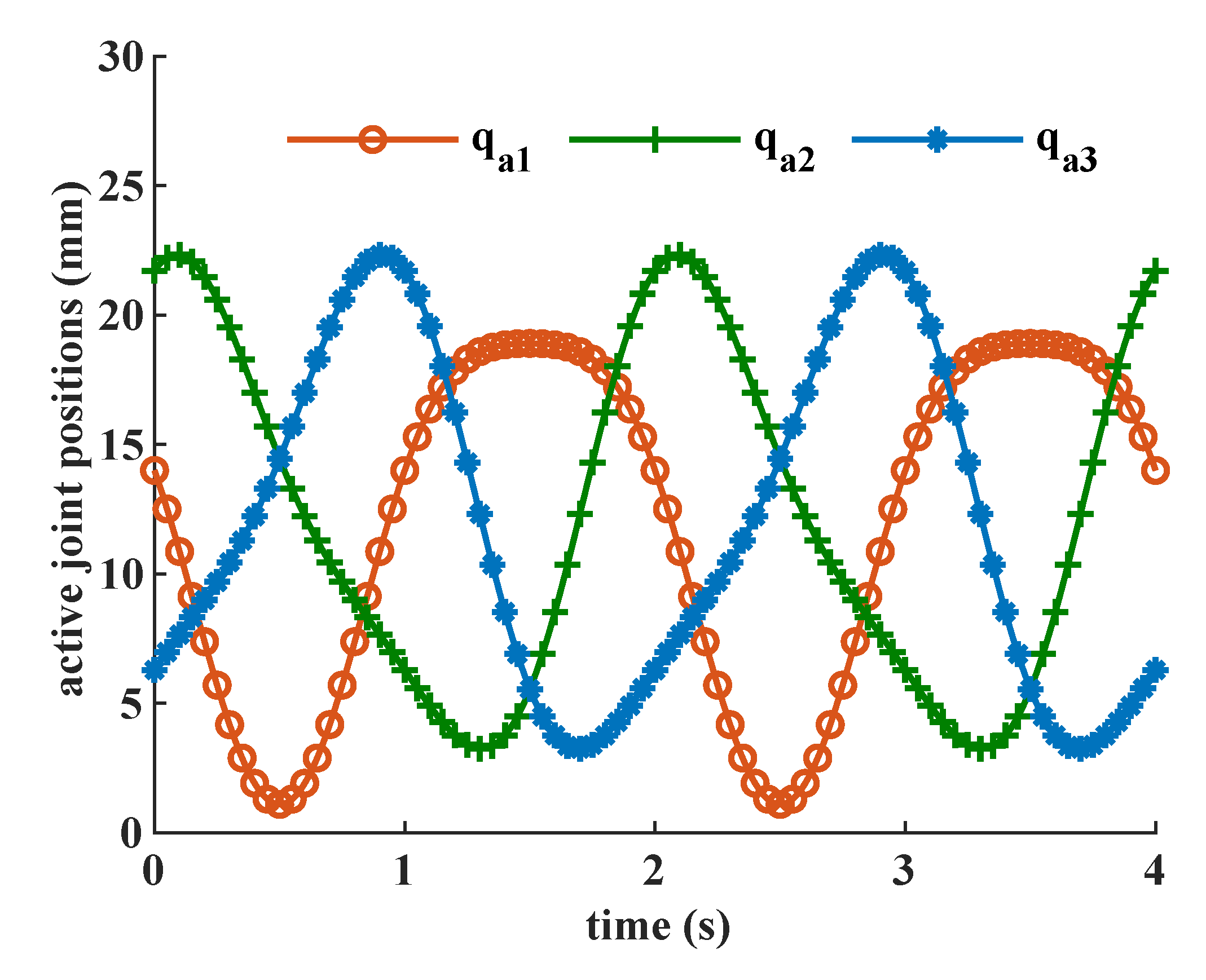
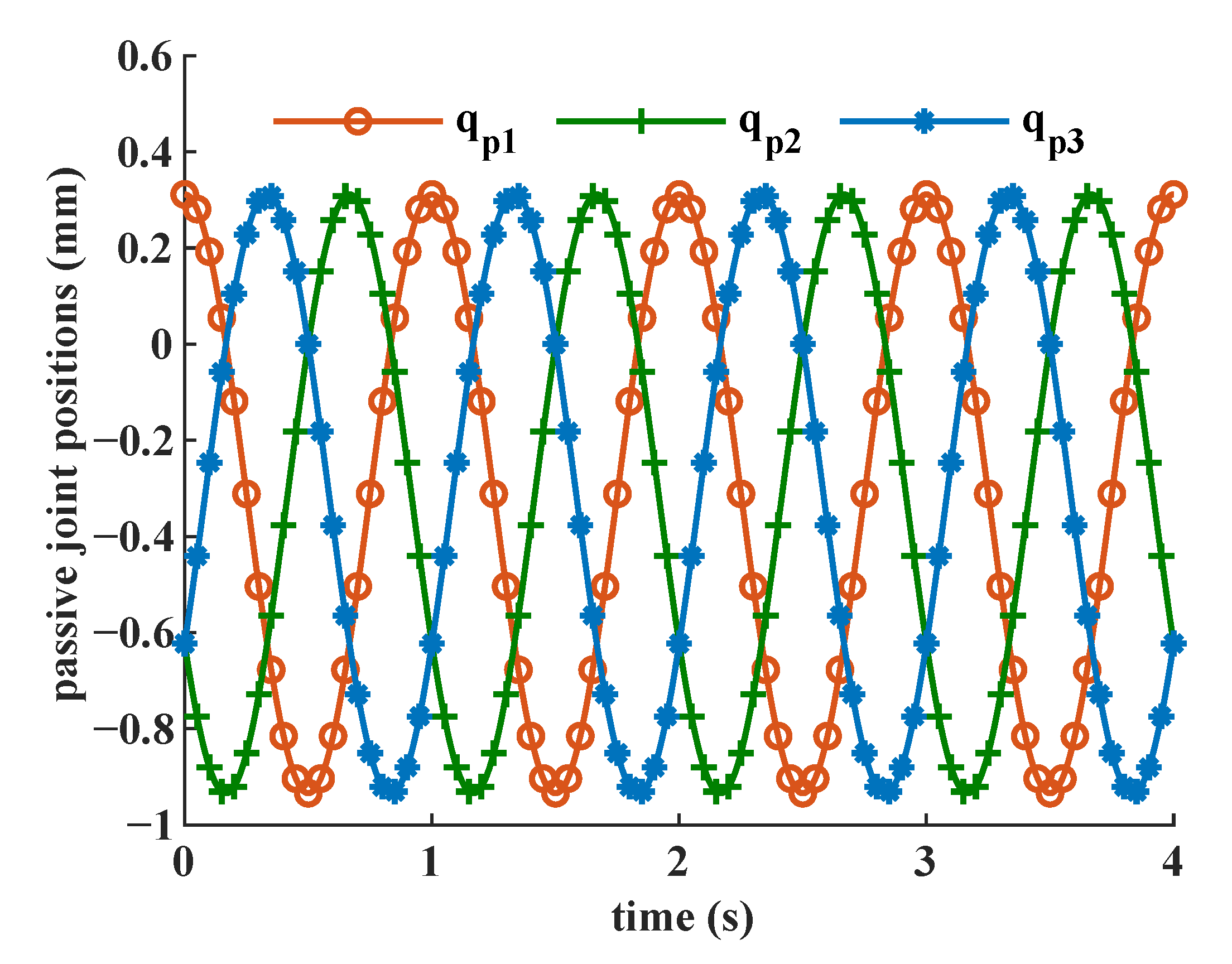
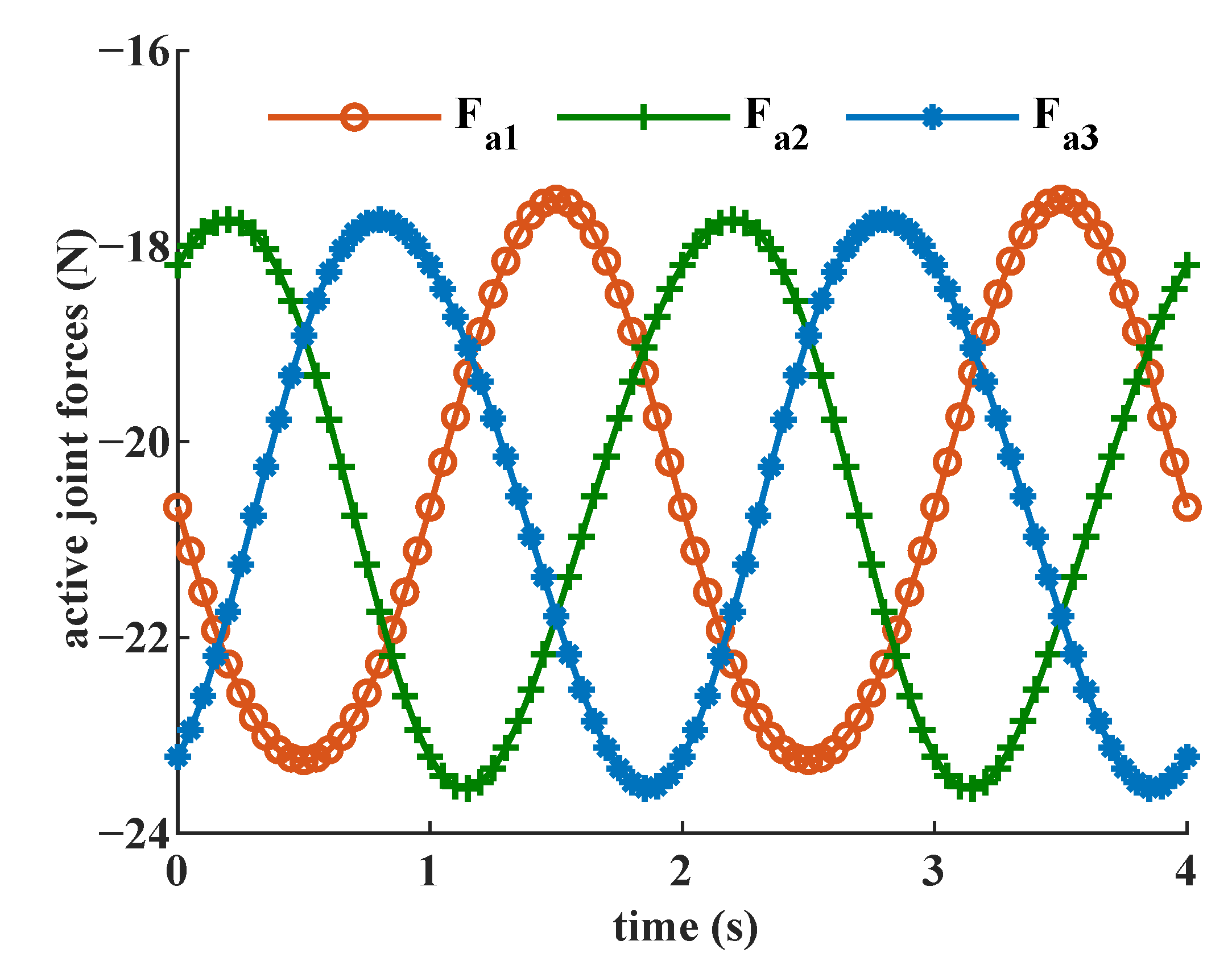
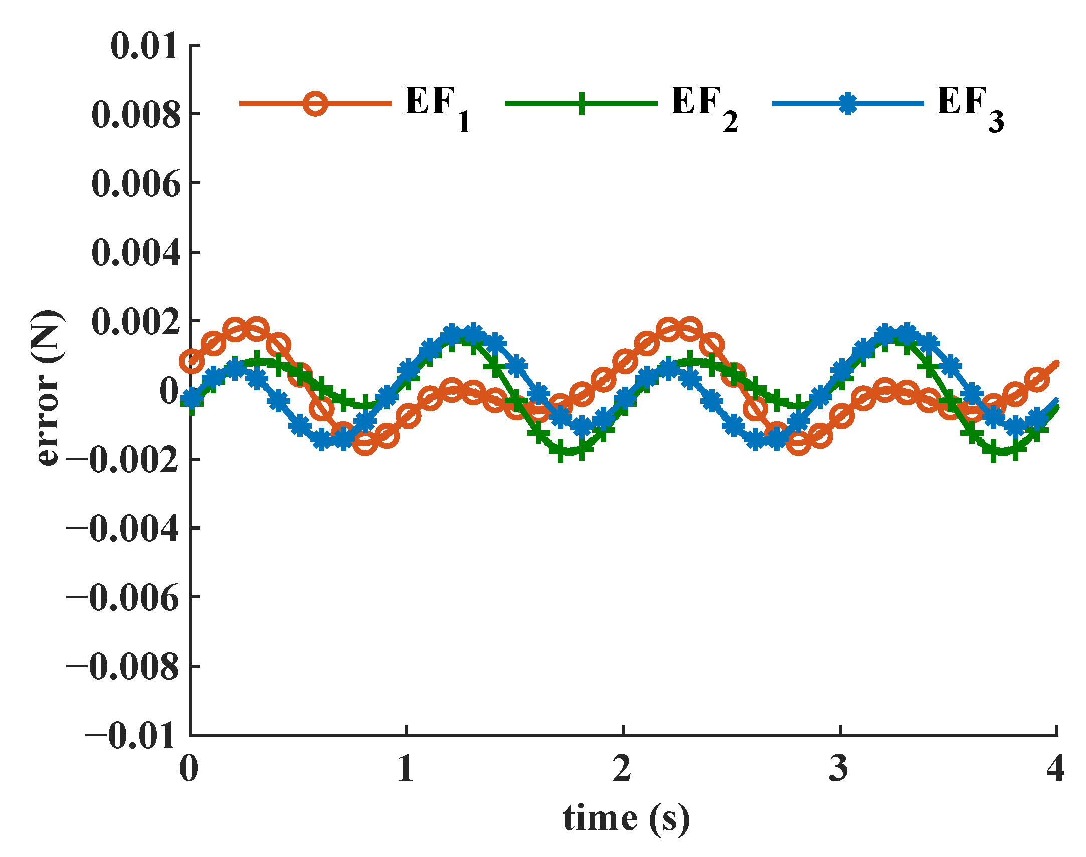
3.2. Simulation Validation

In order to validate the proposed dynamic model, a CAD model of the 2R1T 3PPS PKM prototype with a rigid–flexible structure was developed, and inverse dynamic computation was conducted based on the proposed dynamic model and the commercial dynamic simulation software (SOLIDWORKS software). For inverse dynamic computation of the PKM, a predetermined trajectory of the moving platform is given to determine the required active joint forces in the joint space. The results of required active joint forces obtained from the proposed dynamic model and those from the SOLIDWORKS software are compared. It was assumed that except for three flexure-based passive prismatic joints, each component of the 2R1T 3PPS PKM is a rigid body. The time duration of each trajectory was 4 s with 1 millisecond time step. The direction of gravitational acceleration was along the +Z direction of the base frame. According to the virtual prototype, the key parameters of the 2R1T 3PPS PKM used for dynamic model validation are shown in Table 1.
In our design, the proposed 2R1T 3PPS PKM is employed as a robotic force-controlled end-effector for continuous contact operations. Take typical robotic polishing application for curved surfaces as an example: the required tilting angle of PKM moving platform is larger than 5 , and the required translational range of motion is less than 5 mm. In order to fully cover the designed 2R1T motion DOF of the proposed 2R1T 3PPS PKM, the predetermined trajectory of the moving platform is cone-swing motions for 2R DOF and a cosine motion for 1T DOF which can be described as
u x = cos π t sin 8
u y = sin π t sin 8
M z = 2 × 10 3 cos 2 π t + 195.5 × 10 3
The predetermined trajectory of the moving platform is shown in Figure 6, for which the frequency of cone swing motions is 0.5 Hz, the tilting angle of the PKM moving platform is 8 , and the frequency and the amplitude of the translational motion are 1 Hz and 4 mm, respectively. The corresponding active and passive prismatic joint displacements are shown in Figure 7 and Figure 8, respectively. The ranges of motion of active prismatic joints are within 25 mm, and the ranges of motion of passive prismatic joints are smaller than 1 mm.
As shown in Figure 9, the required active joint forces for the predetermined trajectory were computed based on the derived dynamic model in Equation (47). The periods of three required active joint forces are the same, but the phases are different. The mean values of the required active joint forces are quite close. Figure 10 shows the errors of required active joint forces between computation results from the closed-form dynamic model and SOLIDWORKS software. The results show that they have the same periods but with different patterns. The mean absolute errors (MAEs) of the required active joint forces were 7.7003 × 10 4 N, 7.6048 × 10 4 N, and 8.3248 × 10 4 N, respectively.

4. Coupling-Effects Analysis of the Flexure-Based Passive Prismatic Joints

In the proposed 2R1T 3PPS PKM, as the required displacements of the three passive prismatic joints are as small as few millimeters, the double compound rectilinear flexure mechanisms are employed for the three passive prismatic joints. These flexure-based prismatic joints have the advantages of low moving mass and zero friction. However, the coupling effects of their stiffness and elastic deformation on the PKM’s dynamic behaviors need to be further investigated.

4.1. Stiffness Model

The proposed 2R1T 3PPS PKM is employed as a robotic force-controlled end-effector. The required operation speed is relatively low compared to that of pick-and-place application. The flexure-based passive prismatic joints employ double compound rectilinear flexures, which are designed with large enough ranges of motion and high off-axis stiffness ratios. As such, only the stiffness and deformation in driving directions of the flexure-based passive prismatic joints are uniformly taken into consideration. The stiffness in driving directions (x-axis) of the double compound rectilinear flexure is determined by
K x = 2 E b h 3 L 3
where E is the Young’s modulus of the material, L is the leaf length, h is the leaf width, and b is the thickness of the plate.
The stiffness model of the flexure was verified through FEA and shows good agreement with the simulation results. In the allowed range of motion, the stiffness in driving directions (x axis) of the double compound rectilinear flexure is constant with proper design.

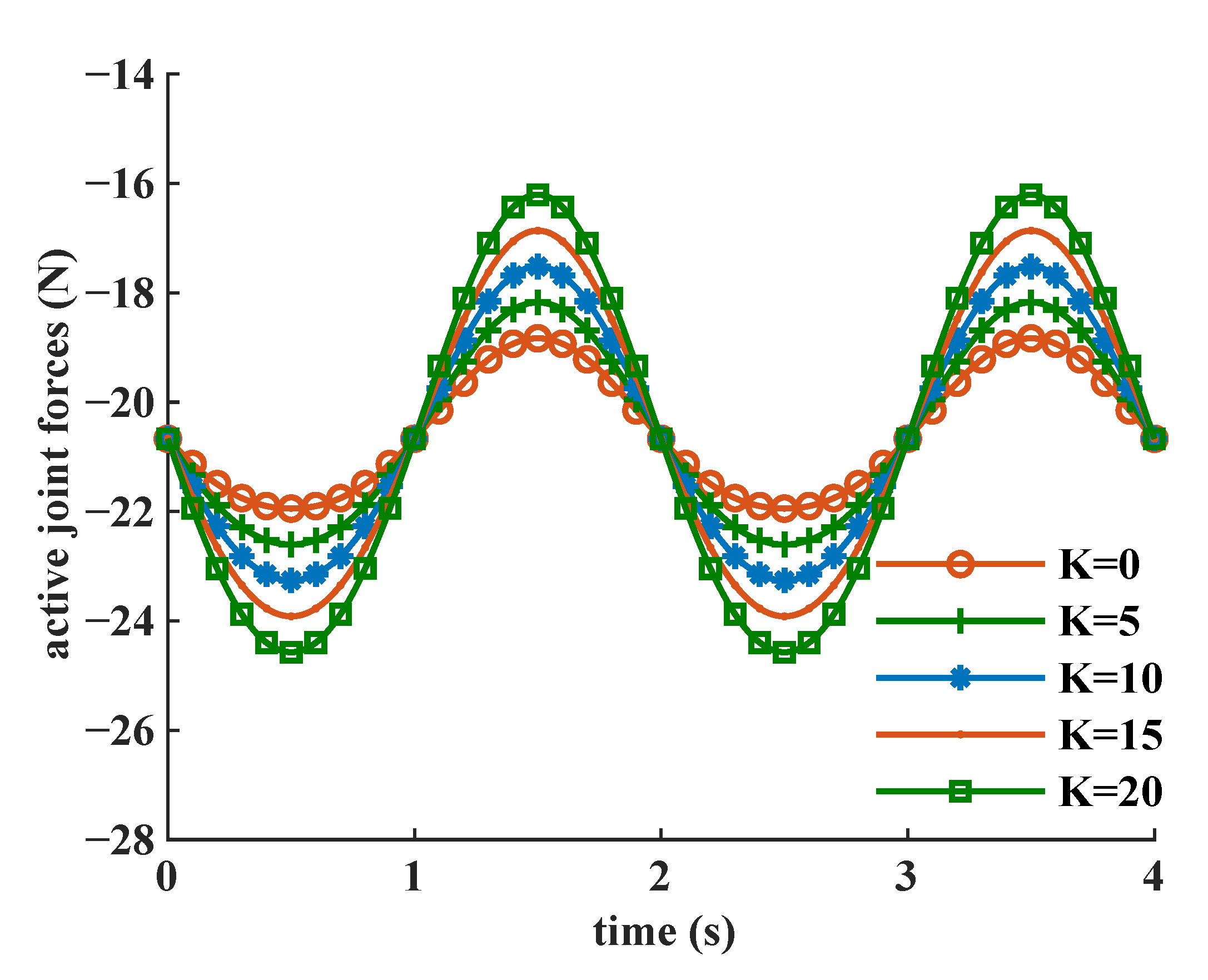
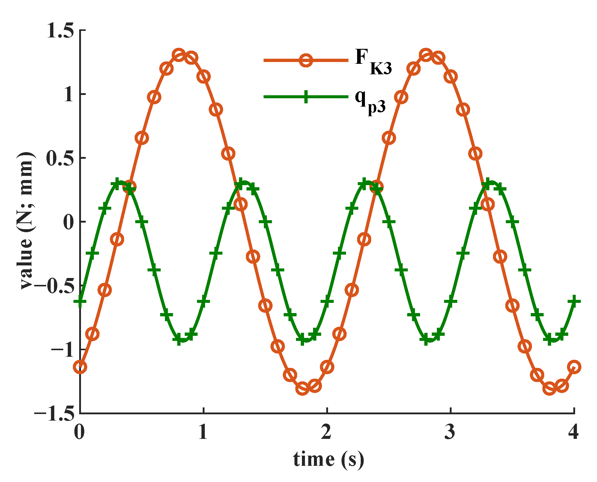
4.2. Coupling Effects on Dynamic Behavior

Based on the closed-form dynamic model, the active joint force can be readily analyzed and interpreted from a physical point of view, which is hardly possible with commercial dynamic analysis software. The inertial forces, the Coriolis and centrifugal forces, the gravitational forces, and the stiffness-related forces can be determined from Equation (47).
In order to investigate the coupling effects of different flexure stiffness on the required active joint force, a simulation computation was conducted. The stiffness range was set to be between 0 N/mm and 20 N/mm. Figure 11 shows the required active joint forces of the same predetermined trajectory change under different flexure stiffness levels. As the flexure stiffness increases from 0 N/mm to 20 N/mm, the trends of required active forces remain the same while the maximum absolute active force changes from 21.95 N to 24.57 N, which indicates that smaller flexure stiffness in driving directions will can reduce the required actuating forces. The simulation results are necessary for the design optimization of the proposed 2R1T 3PPS PKM with a rigid–flexible structure.

5. Discussion

As shown in Figure 10, the results obtained from the closed-form dynamic model show good agreement with those obtained from simulation software, which validates the correctness of the derived closed-form dynamic model. It is observed that small errors still exist in the results of the derived dynamic model, which are mainly due to the truncation errors of parameter values and the cumulative errors during the computation. The derived closed-form dynamic model can be utilized as a fundamental tool for robot design, trajectory planning, and model-based control algorithms.
For the trajectory of the moving platform described in Equations (52)–(54), the result shown in Figure 11 shows that the use of flexure-based passive prismatic joints results in a slight increase in the required active joint force, which also indicates that less flexure stiffness in driving directions is desired. Moreover, the stiffness in driving directions can be adjusted according to various applications without having a severe influence on the required actuator forces.
Based on the closed-form dynamic model, the stiffness-related forces can be extracted from the total required active joint forces. Figure 12, Figure 13 and Figure 14 show the stiffness-related force components of a single active force and the corresponding flexure-based passive prismatic joint displacement. For this specific trajectory described in Equations (52)–(54), the frequency of stiffness-related force component is half of that of the corresponding flexure-based passive prismatic joint displacement which shares the same pattern, as shown in Figure 7 and Figure 8. The amplitudes of the stiffness-related force components are relatively low, which indicates only small influences are introduced on the required active forces.

6. Conclusions

This work proposes a systematic and structured method for formulating the closed-form dynamic model of the 2R1T 3PPS PKM with a rigid–flexible structure. Based on the unique zero-torsion motion characteristic of the 2R1T 3PPS PKM, a symbolic formulation approach was employed to derive the moving platform pose, which is described with linear polynomials of both active and passive prismatic joint variables. Therefore, in order to simplify the formation of a closed-form dynamic model, both active and passive prismatic joint variables were chosen as the quasi-coordinates. Firstly, a closed-form dynamic model in terms of quasi-coordinates was established with a Lagrangian formulation, in which the stiffness and deformation of the three flexure-based passive prismatic joints are uniformly taken into consideration. Then, the principle of virtual work and the relationships between the active and passive prismatic joint variables were employed to eliminate the passive prismatic joint variables. The closed-form dynamic model in terms of active prismatic joint variables was finally obtained. The derived closed-form dynamic model was validated by the comparison with the simulation results obtained from commercial dynamic simulation software. The mean absolute errors of the three required active joint forces between the proposed dynamic model and commercial software are as small as 7.7003 × 10 4 , 7.6048 × 10 4 , and 8.3248 × 10 4 N. Based on the derived closed-form dynamic model, the effects of different flexure stiffness in driving directions on the required active joint force were investigated, which indicate that a smaller flexure stiffness in driving directions is desired. Future work will be focused on the experimental validation of proposed closed-form dynamic model and development of dynamic model-based force control algorithms.

Author Contributions

Conceptualization, G.Y. and Z.F.; methodology, R.Z.; software, R.Z.; validation, R.Z.; formal analysis, R.Z.; investigation, R.Z. and H.L.; resources, H.L.; data curation, R.Z.; writing—original draft preparation, R.Z.; writing—review and editing, G.Y., Z.F. and C.-Y.C.; visualization, R.Z.; supervision, G.Y. and Z.F.; project administration, G.Y.; funding acquisition, G.Y., Z.F., C.-Y.C. and C.Z. All authors have read and agreed to the published version of the manuscript.

Funding

This research was funded by the National Key Research and Development Program of China (2022YFB4702500), the National Natural Science Foundation of China (92048201, U1909215, 52127803), the Ningbo Key Project of Scientific and Technological Innovation 2025 (2021Z020, 2021Z093), and the Key Research and Development Program of Zhejiang (2022C01096).

Institutional Review Board Statement

Not applicable.

Informed Consent Statement

Not applicable.

Data Availability Statement

Not applicable.

Acknowledgments

The authors are very thankful to the support of the National Key Research and Development Program of China (2022YFB4702500), the National Natural Science Foundation of China (92048201, U1909215, 52127803), the Ningbo Key Project of Scientific and Technological Innovation 2025 (2021Z020, 2021Z093), and the Key Research and Development Program of Zhejiang (2022C01096).

Conflicts of Interest

The authors declare no conflict of interest.

Abbreviations

The following abbreviations are used in this manuscript:
PKMParallel kinematic mechanism
3PPS3-legged prismatic-prismatic-spherical
MAEMean absolute error
2R1TTwo rotational and one translational

References

  1. Merlet, J.P. Parallel Robots; Springer Science and Business Media: Dordrecht, Netherlands, 2006; Volume 128. [Google Scholar]
  2. Liping, W.; Huayang, X.; Liwen, G. Kinematics and inverse dynamics analysis for a novel 3-PUU parallel mechanism. Robotica 2017, 35, 2018–2035. [Google Scholar] [CrossRef]
  3. Liu, X.J.; Wang, J. Parallel Kinematics; Springer Tracts in Mechanical Engineering; Springer Tracts in Mechanical Engineering: Berlin/Heidelberg, Germany, 2014. [Google Scholar]
  4. Wang, D.; Wang, L.; Wu, J.; Ye, H. An Experimental Study on the Dynamics Calibration of a 3-DOF Parallel Tool Head. IEEE/ASME Trans. Mechatronics 2019, 24, 2931–2941. [Google Scholar] [CrossRef]
  5. Valles, M.; Diaz-Rodriguez, M.; Valera, A.; Mata, V.; Page, A. Mechatronic Development and Dynamic Control of a 3-DOF Parallel Manipulator. Mech. Based Des. Struct. Mech. 2012, 40, 434–452. [Google Scholar] [CrossRef]
  6. Oba, Y.; Yamada, Y.; Igarashi, K.; Katsura, S.; Kakinuma, Y. Replication of skilled polishing technique with serial–parallel mechanism polishing machine. Precis. Eng. 2016, 45, 292–300. [Google Scholar] [CrossRef]
  7. Dasgupta, B.; Choudhury, P. A general strategy based on the Newton–Euler approach for the dynamic formulation of parallel manipulators. Mech. Mach. Theory 1999, 34, 801–824. [Google Scholar] [CrossRef]
  8. Guo, F.; Cheng, G.; Pang, Y. Explicit dynamic modeling with joint friction and coupling analysis of a 5-DOF hybrid polishing robot. Mech. Mach. Theory 2022, 167, 104509. [Google Scholar] [CrossRef]
  9. Marques, F.; Roupa, I.; Silva, M.T.; Flores, P.; Lankarani, H.M. Examination and comparison of different methods to model closed loop kinematic chains using Lagrangian formulation with cut joint, clearance joint constraint and elastic joint approaches. Mech. Mach. Theory 2021, 160, 104294. [Google Scholar] [CrossRef]
  10. Xin, G.; Deng, H.; Zhong, G. Closed-form dynamics of a 3-DOF spatial parallel manipulator by combining the Lagrangian formulation with the virtual work principle. Nonlinear Dyn. 2016, 86, 1329–1347. [Google Scholar] [CrossRef]
  11. Abo-Shanab, R.F. Dynamic modeling of parallel manipulators based on Lagrange–D’Alembert formulation and Jacobian/Hessian matrices. Multibody Syst. Dyn. 2020, 48, 403–426. [Google Scholar] [CrossRef]
  12. Kane, T.R.; Levinson, D.A. The Use of Kane’s Dynamical Equations in Robotics. Int. J. Robot. Res. 1983, 2, 3–21. [Google Scholar] [CrossRef]
  13. Wang, J.T.; Huston, R.L. Kane’s Equations With Undetermined Multipliers—Application to Constrained Multibody Systems. J. Appl. Mech. 1987, 54, 424–429. [Google Scholar] [CrossRef]
  14. Tsai, L.W. Solving the Inverse Dynamics of a Stewart-Gough Manipulator by the Principle of Virtual Work. J. Mech. Des. 1999, 122, 3–9. [Google Scholar] [CrossRef]
  15. Kalani, H.; Rezaei, A.; Akbarzadeh, A. Improved general solution for the dynamic modeling of Gough–Stewart platform based on principle of virtual work. Nonlinear Dyn. 2016, 83, 2393–2418. [Google Scholar] [CrossRef]
  16. Lu, S.; Ding, B.; Li, Y. Minimum-jerk trajectory planning pertaining to a translational 3-degree-of-freedom parallel manipulator through piecewise quintic polynomials interpolation. Adv. Mech. Eng. 2020, 12, 1–18. [Google Scholar] [CrossRef]
  17. Sandor, G.N.; Zhuang, X. A linearized lumped parameter approach to vibration and stress analysis of elastic linkages. Mech. Mach. Theory 1985, 20, 427–437. [Google Scholar] [CrossRef]
  18. Liang, D.; Song, Y.; Sun, T.; Jin, X. Rigid–flexible coupling dynamic modeling and investigation of a redundantly actuated parallel manipulator with multiple actuation modes. J. Sound Vib. 2017, 403, 129–151. [Google Scholar] [CrossRef]
  19. Ma, Y.; Liu, H.; Zhang, M.; Li, B.; Liu, Q.; Dong, C. Elasto-dynamic performance evaluation of a 6-DOF hybrid polishing robot based on kinematic modeling and CAE technology. Mech. Mach. Theory 2022, 176, 104983. [Google Scholar] [CrossRef]
  20. Zheng, K.M.; Hu, Y.M.; Yu, W.Y. A novel parallel recursive dynamics modeling method for robot with flexible bar-groups. Appl. Math. Model. 2020, 77, 267–288. [Google Scholar] [CrossRef]
  21. Liao, S.; Ding, B.; Li, Y. Design, Assembly, and Simulation of Flexure-Based Modular Micro-Positioning Stages. Machines 2022, 10, 421. [Google Scholar] [CrossRef]
  22. Yang, C.; Li, Q.C.; Chen, Q.H. Natural frequency analysis of parallel manipulators using global independent generalized displacement coordinates. Mech. Mach. Theory 2021, 156, 104145. [Google Scholar] [CrossRef]
  23. Xiao, L.J.; Yan, F.P.; Chen, T.X.; Zhang, S.S.; Jiang, S. Study on nonlinear dynamics of rigid-flexible coupling multi-link mechanism considering various kinds of clearances. Nonlinear Dyn. 2022, 111, 3279–3306. [Google Scholar] [CrossRef]
  24. Zhang, Z.Q.; Wang, L.; Liao, J.N.; Zhao, J.; Yang, Q. Rigid-flexible coupling dynamic modeling and performance analysis of a bioinspired jumping robot with a six-bar leg mechanism. J. Mech. Sci. Technol. 2021, 35, 3675–3691. [Google Scholar] [CrossRef]
  25. Beiranvand, A.; Kalhor, A.; Masouleh, M.T. Modeling, identification and minimum length integral sliding mode control of a 3-DOF cartesian parallel robot by considering virtual flexible links. Mech. Mach. Theory 2021, 157, 104183. [Google Scholar] [CrossRef]
  26. Liang, D.; Song, Y.; Sun, T.; Jin, X. Dynamic modeling and hierarchical compound control of a novel 2-DOF flexible parallel manipulator with multiple actuation modes. Mech. Syst. Signal Process. 2018, 103, 413–439. [Google Scholar] [CrossRef]
  27. Guo, F.; Cheng, G.; Wang, S.; Li, J. Rigid–flexible coupling dynamics analysis with joint clearance for a 5-DOF hybrid polishing robot. Robotica 2022, 40, 2168–2188. [Google Scholar] [CrossRef]
  28. Teo, T.J.; Yang, G.; Chen, I.M. A large deflection and high payload flexure-based parallel manipulator for UV nanoimprint lithography: Part I. Modeling and analyses. Precis. Eng. 2014, 38, 861–871. [Google Scholar] [CrossRef]
  29. Teo, T.J.; Chen, I.M.; Yang, G. A large deflection and high payload flexure-based parallel manipulator for UV nanoimprint lithography: Part II. Stiffness modeling and performance evaluation. Precis. Eng. 2014, 38, 872–884. [Google Scholar] [CrossRef]
  30. Yang, G.; Zhu, R.; Fang, Z.; Chen, C.; Zhang, C. Kinematic Design of a 2R1T Robotic End-Effector with Flexure Joints. IEEE Access 2020, 8, 57204–57213. [Google Scholar] [CrossRef]
  31. Zhu, R.; Yang, G.; Fang, Z.; Dai, J.; Chen, C.Y.; Zhang, G.; Zhang, C. Hybrid orientation/force control for robotic polishing with a 2R1T force-controlled end-effector. Int. J. Adv. Manuf. Technol. 2022, 121, 2279–2290. [Google Scholar] [CrossRef]
  32. Craig, J.J. Introduction to Robotics: Mechanics and Control, 4th ed.; Pearson: London, UK, 2018. [Google Scholar]
Figure 1. The prototype of the 2R1T 3PPS PKM as a force-controlled end-effector.
Machines 11 00260 g001
Figure 2. Kinematic diagram of the proposed 2R1T 3PPS PKM.
Machines 11 00260 g002
Figure 3. Equivalent rotation about a unit axis k parallel to the base plate.
Machines 11 00260 g003
Figure 4. The derivation process of the proposed dynamic modeling approach.
Machines 11 00260 g004
Figure 5. The sketch representing the body frames of the virtual isolated bodies.
Machines 11 00260 g005
Figure 6. Desired motion for the moving platform of the 2R1T 3PPS PKM.
Machines 11 00260 g006
Figure 7. Desired motion for the active joints of the 2R1T 3PPS PKM.
Machines 11 00260 g007
Figure 8. Desired motion for the passive joints of the 2R1T 3PPS PKM.
Machines 11 00260 g008
Figure 9. Required active joint forces computed from the proposed dynamic model.
Machines 11 00260 g009
Figure 10. The errors of required active joint forces between model computation and software simulation.
Machines 11 00260 g010
Figure 11. Required active joint forces of the same predetermined trajectory with different flexure stiffness levels.
Machines 11 00260 g011
Figure 12. Stiffness-related component, F K 1 , of the required active force, and the corresponding flexure-based passive prismatic joint displacement q p 1 .
Machines 11 00260 g012
Figure 13. Stiffness-related component, F K 2 , of the required active force, and the corresponding flexure-based passive prismatic joint displacement q p 2 .
Machines 11 00260 g013
Figure 14. Stiffness-related component, F K 3 , of the required active force, and the corresponding flexure-based passive prismatic joint displacement q p 3 .
Machines 11 00260 g014
Table 1. Simulation parameters of the 3PPS PKM for dynamic model’s validation.
ParameterValueUnit
Acceleration of gravity g9.80665 m / s 2
Mass of active joints m 1 , 2 , 3 1264.25865111g
Mass of passive joints m 4 , 5 , 6 140.13865914g
Mass of moving platform m 7 2066.84394668g
Moment of inertia I 7 c o m x x 7.003898473 × 10 3 kg · m 2
Moment of inertia I 7 c o m y y 7.004407761 × 10 3 kg · m 2
Moment of inertia I 7 c o m z z 3.256238466 × 10 3 kg · m 2
Moment of inertia I 7 c o m x y 0.701 × 10 9 kg · m 2
Moment of inertia I 7 c o m x z 3.111 × 10 9 kg · m 2
Moment of inertia I 7 c o m y z 0.439 × 10 9 kg · m 2
Local coordinates of body 7 COM 0 , 0 , 64.81 mm
Circumcircle radius r64 mm
Initial distance H B M 183.5 mm
Flexure stiffness k s i 10 N / mm
Disclaimer/Publisher’s Note: The statements, opinions and data contained in all publications are solely those of the individual author(s) and contributor(s) and not of MDPI and/or the editor(s). MDPI and/or the editor(s) disclaim responsibility for any injury to people or property resulting from any ideas, methods, instructions or products referred to in the content.

