Article

Fault Diagnosis of Rotating Machinery Based on Two-Stage Compressed Sensing

1
College of Mechanical and Vehicle Engineering, Chongqing University, Chongqing 400044, China
2
College of Electrical Engineering, Henan University of Technology, Zhengzhou 450001, China
*
Author to whom correspondence should be addressed.
Machines 2023, 11(2), 242; https://doi.org/10.3390/machines11020242
Submission received: 26 December 2022 / Revised: 31 January 2023 / Accepted: 2 February 2023 / Published: 6 February 2023

Abstract

:
Intelligent on-site fault diagnosis and professional vibration analysis are essential for the safety and stability of rotating machinery operation. This paper represents a fault diagnosis scheme based on two-stage compressed sensing for triaxial vibration data, which realizes fault diagnosis for rotating machinery based on compressed data and data reconstruction for professional vibration analysis. In the 1st stage, the triaxial vibration signals are compressed using a pre-designed hybrid measurement matrix; these compressed data can be used both for time-frequency transform and for vibration data reconstruction. In the 2nd stage, the frequency spectra of the triaxial vibration signals are fused and further compressed using another pre-designed joint measurement matrix, which inhibits the high-frequency noises simultaneously. Finally, the fused spectra are employed as feature vectors in sparse-representation-based classification, where the proposed batch matching pursuit (BMP) algorithm is utilized to calculate the sparse vectors. The two-stage compression scheme and the BMP algorithm minimize the computational cost of on-site fault diagnosis, which is suitable for edge computing platforms. Meanwhile, the compressed vibration data can be reconstructed, which provides evidence for professional vibration analysis. The method proposed in this study is validated by two practical case studies, in which the accuracies are 99.73% and 96.70%, respectively.

1. Introduction

Fault diagnosis improves the safety, reliability, and maintenance efficiency of rotating machinery, and vibration signal analysis is one of the most popular diagnosis techniques. Many novel methods and indexes are proposed for rotating machinery based on vibration signals, such as feature mode decomposition [1], iterative adaptive crucial mode decomposition [2], Gini index [3], and neural network-based methods [4]. These methods provide remarkable performance for fault diagnosis. Meanwhile, emerging technologies such as edge computing and industrial internet of things are widely used in mechanical systems, based on triaxial vibration data. Intelligent fault diagnosis implemented in edge computing platform is becoming a promising supplement for vibration analysts’ professional analysis. Considering the computational capability of the edge computing platform, combined with the effects of triaxial vibration data fusion and reduction, the promotion of algorithm efficiency is essential for on-site fault diagnosis. Meanwhile, for the diagnosis of some intractable faults, original vibration data is the fundamental for the calculation of effective indexes such as sparsity indexes [5]. Alternatively, professional vibration analysis is required, in which case data reconstruction is also necessary [6]. Thus, a triaxial vibration data processing scheme which integrates data compression, data reconstruction, data denoising, and data fusion [7] into high-efficiency fault diagnosis is essential for practical engineering applications. Fortunately, compressed sensing provides an efficient data compression and reconstruction tool for fault diagnosis. Fault diagnosis based on compressed sensing has been an emerging research field in the past few years, and related research mainly focus on dictionary matrix construction and learning, feature extraction of compressed data, and the combination with machine learning [8], etc.
First, the dictionary learning or dictionary matrix construction improves the robustness or accuracy of fault diagnosis. In Ref. [9], an adaptive compressed sensing method is presented to identify a weak fault signature and improve fault diagnosis accuracy, in which the dictionary learning method is employed. In Ref. [10], a dictionary matrix composed of labeled samples acquired from different conditions is constructed, which improves the robustness of fault diagnosis. However, few dictionary matrices can currently integrate the fault sensitive information of all triaxial vibration signals, even though in practice, most of the rotating machinery monitoring systems contain vertical, horizontal, and axial vibration sensors.
Next, to improve the computational efficiency, fault sensitive features are extracted in the compressed domain. For example, in Ref. [11], weak fault features are extracted based on wavelet packet decomposition and particle swarm optimization. In Ref. [12], wavelet packet energy entropy is extracted from the compressed data, and then used as features for sparse autoencoder. In these studies, a random matrix is employed as the measurement matrix. However, the frequency characteristics of the original vibration signals are destroyed: thus, the widely-used and edge computing-friendly time-frequency transform cannot be applied to these compressed data.
The combination of compressed sensing and machine learning reduces the pressure of data transmission, storage and calculation of machine learning. In Ref. [13], a fault diagnosis approach which combines a Teager energy operator demodulation and deep autoencoder of compressed sensing is proposed, which improves the fault diagnosis robustness and accuracy. In Ref. [14], a fault diagnosis scheme based on compressed sensing theory and an improved multi-scale neural network is presented, where compressed sensing is employed for data reduction. However, machine learning, especially deep learning, requires powerful computational capability of the computation platform, which poses a challenge for its application in on-site and real-time fault diagnosis.
The three fundamental elements of compressed sensing are: measurement matrix design, dictionary matrix construction, and sparse vector calculation [15]. The existing fault diagnosis methods based on compressed sensing mainly involve a dictionary matrix construction [16] and a sparse vector calculation: few compressed-sensing-based fault diagnosis methods focus specifically on the design of an expressly appropriate measurement matrix for triaxial vibration data which would aim to retain frequency characteristics and reduce high-frequency noise, as well as enabling multisource fusion. Yet, these issues are critical in practical engineering. Meanwhile, the combination of high-rate compression and data reconstruction for vibration data processing is also a bottleneck issue, since full original vibration data storage and transmission are expensive, while data reconstruction can hardly be realized in traditional feature extraction methods.
To solve the above problems, in this study, considering the synergy of the on-site intelligent diagnosis implemented in an edge computing platform and the professional analysis based on original vibration data and compressed sensing, a new fault diagnosis scheme is proposed, which contains a two-stage compression scheme, exclusive design of the measurement matrices, and batch matching pursuit algorithm. The main contributions of this study are summarized as follows.
(1)
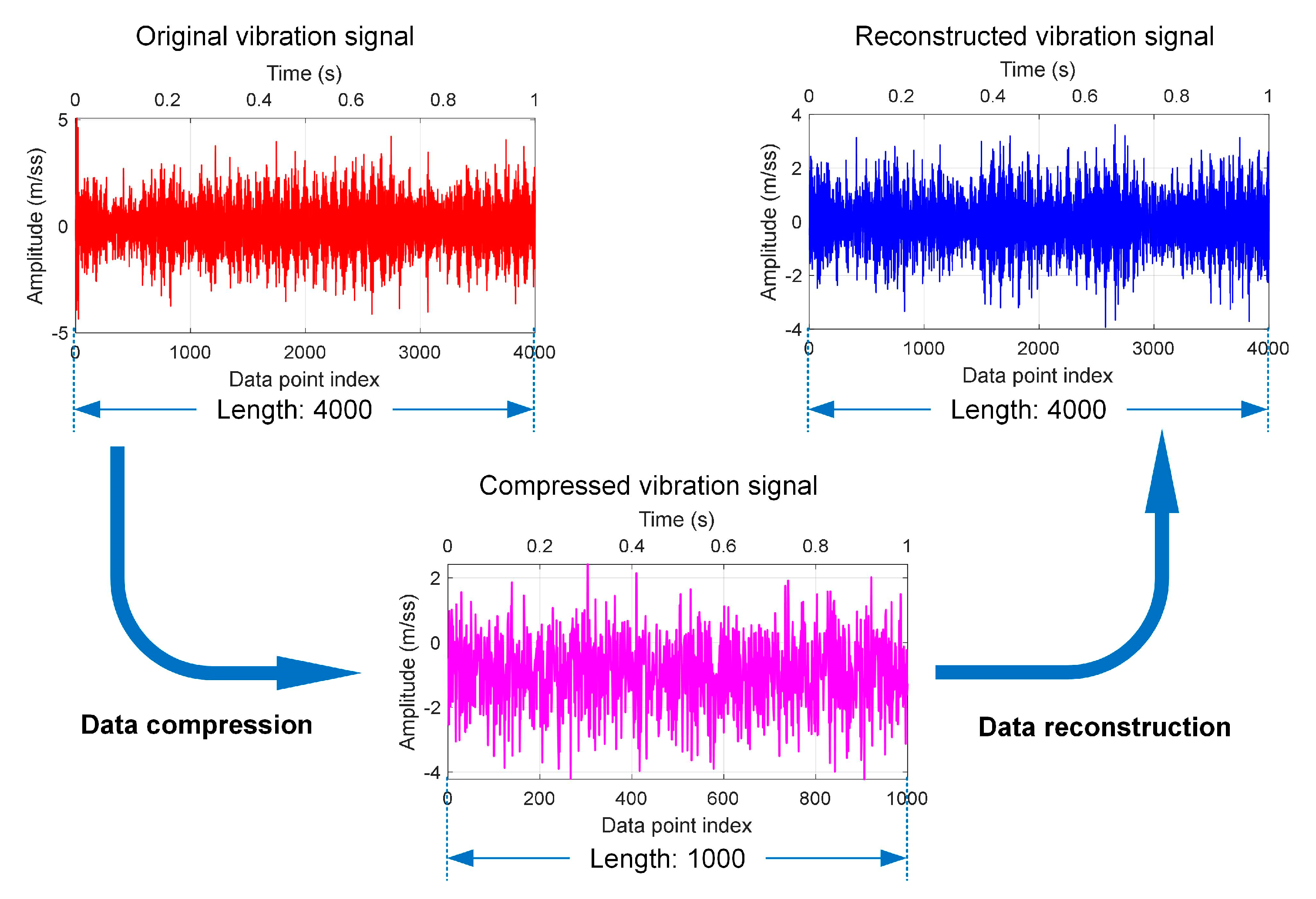
The proposed two-stage compression scheme provides an extremely high data compression efficiency for on-site fault diagnosis, while the original vibration data can be reconstructed for professional vibration analysis.
(2)
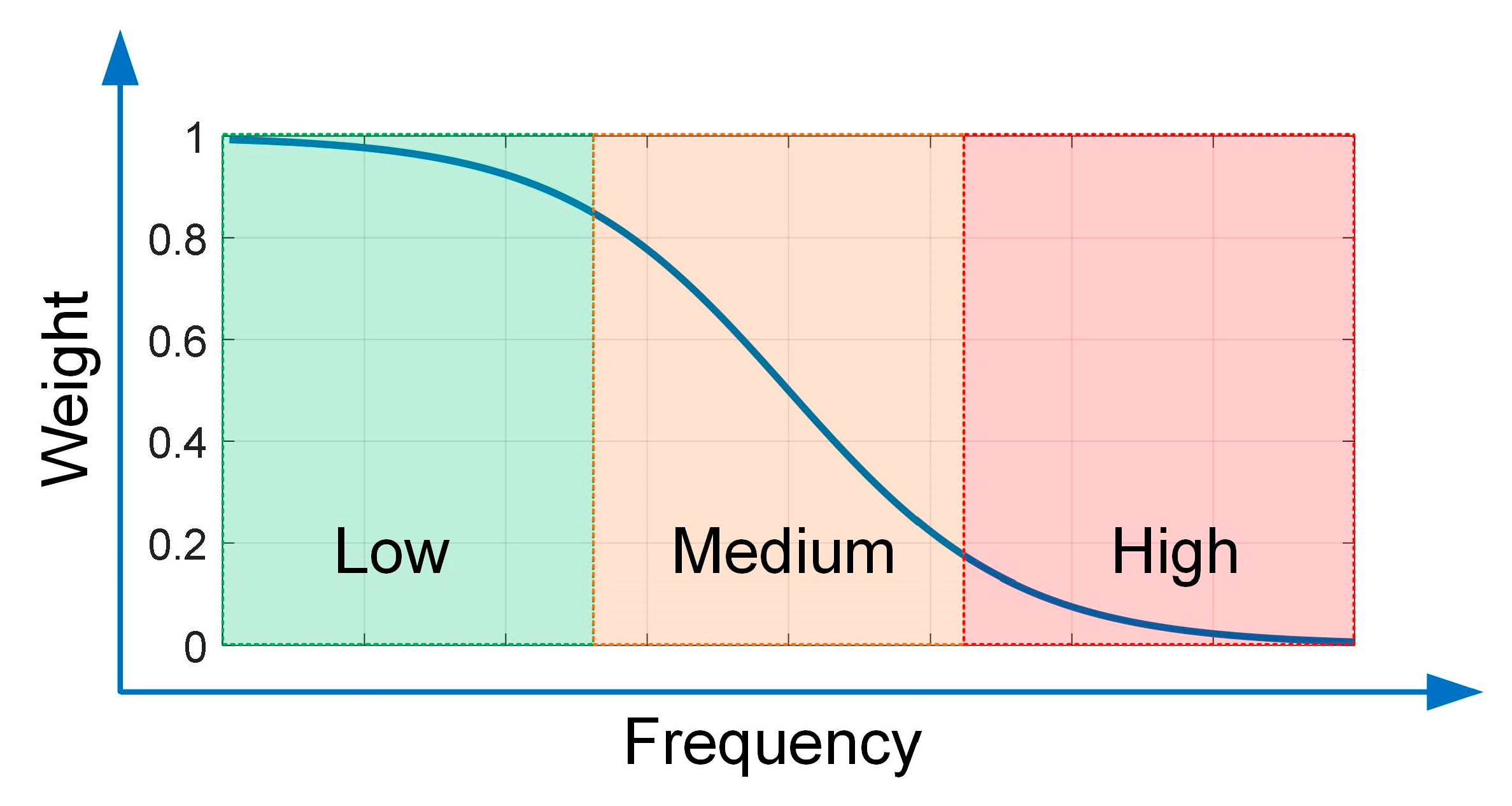
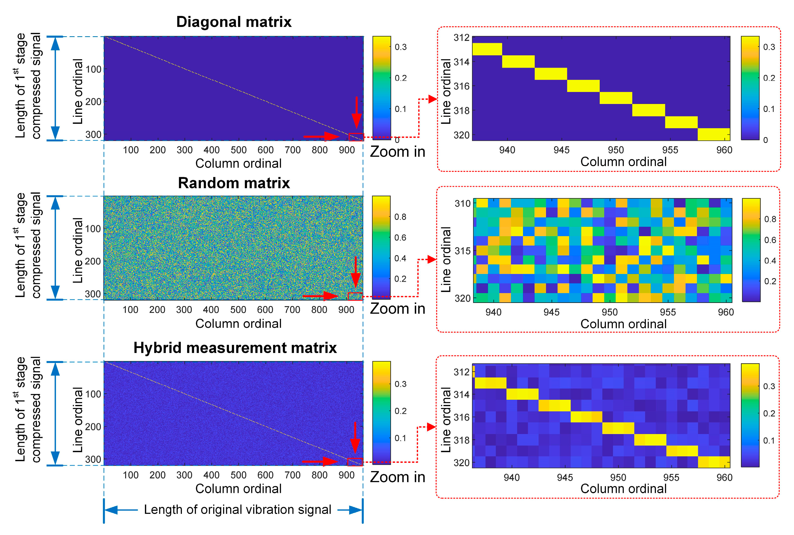
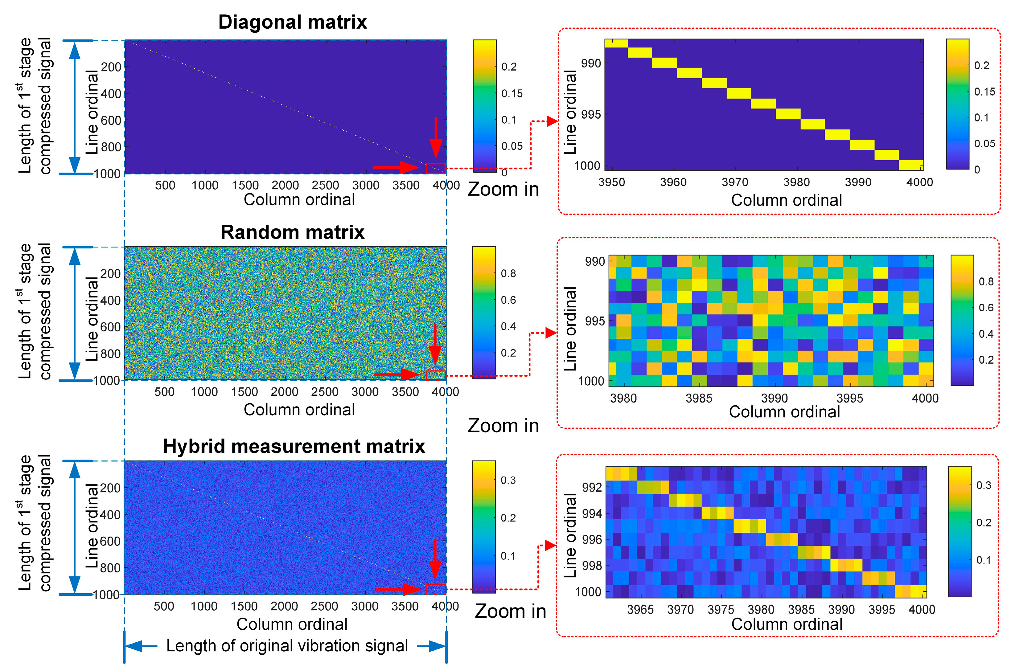
Novel measurement matrices are designed for fault diagnosis based on compressed sensing, which emphasize retention of frequency characteristics, high-frequency noise reduction, and multisource data fusion.
(3)
For sparse representation-based classification, a batch match pursuit algorithm is proposed, which improves the efficiency of sparse vector calculation in sparse representation.
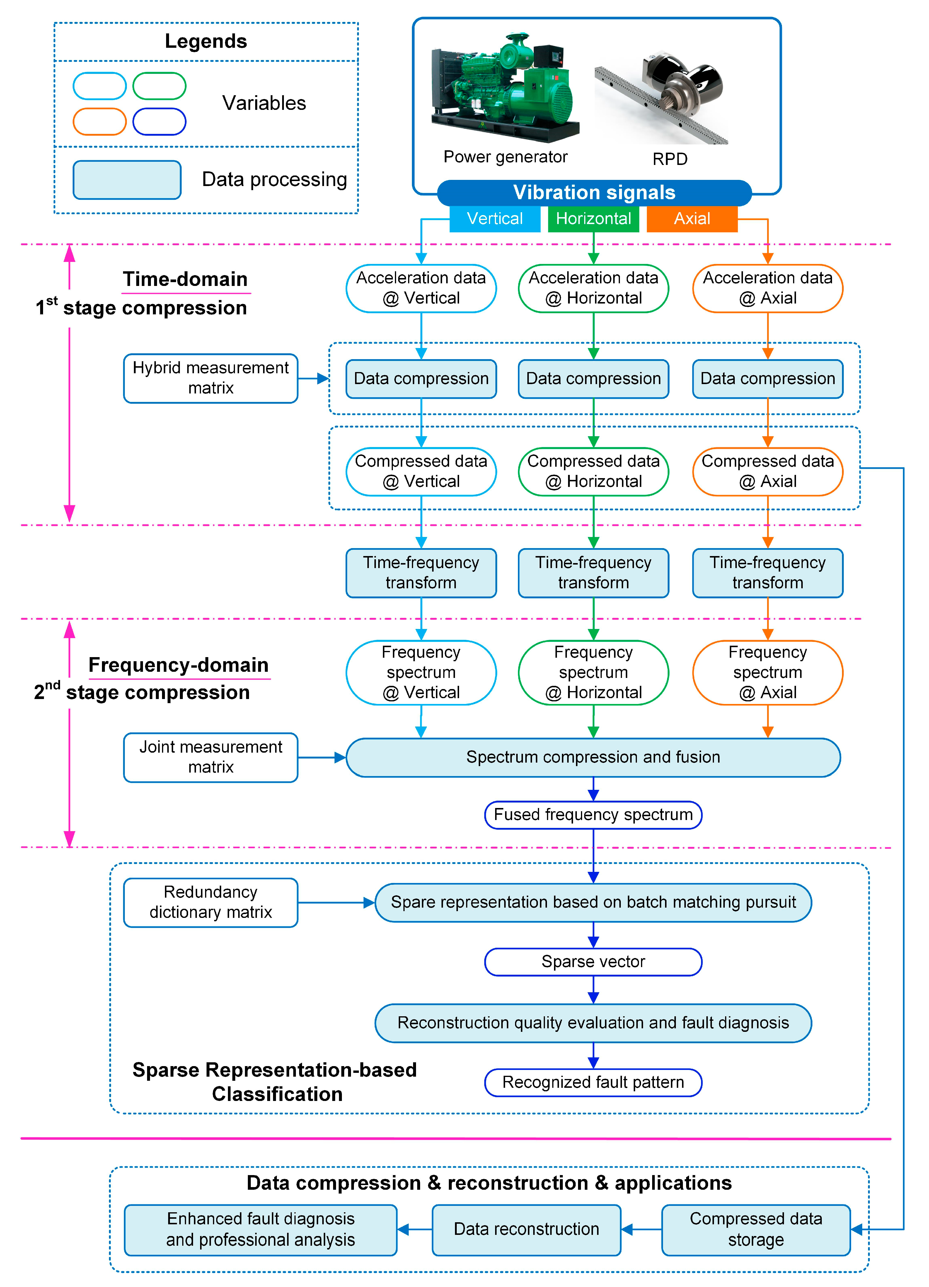
The subsequent sections of this paper are arranged as follows. In Section 2, the architecture and the details of the fault diagnosis method are presented. In Section 3, the proposed method is validated using two practical cases, including maintenance level recognition of a landfill gas power generator (LGPG) and fault diagnosis of the driving gear in a battery swapping system (BSS). In Section 4, conclusions of this work are drawn, and future work described.

2. Methodology

The structure of the proposed method is shown in Figure 1. In this study, triaxial vibration signals of rotating machinery are acquired, including monitoring data collected from vertical, horizontal and axial vibration sensors, the vibration data are then compressed in two stages: the 1st stage of compression is a time-domain compression, where vibration data acquired from different sensors are respectively compressed; the 2nd stage of compression is a frequency-domain compression, during which the frequency spectra obtained from the triaxial vibration signals are fused. In the 1st stage, to retain the frequency features of the vibration data, a hybrid measurement matrix is designed, which is composed of a diagonal matrix and a random matrix. In the 2nd stage, to fuse the spectra and filter out the high-frequency noises, a joint measurement matrix is designed based on the sigmoid function. Finally, the fused frequency spectrum is employed as the input feature vector of sparse-representation-based classification (SRC), in which the sparse vector is calculated based on the proposed BMP algorithm, and the fault pattern of the testing sample is determined by evaluating the quality of signal reconstruction. Note that considering the randomness of the hybrid measurement matrix, the original vibration data can be reconstructed based on compressed sensing, and these reconstructed data provide evidence for enhanced fault diagnosis, similar to a vibration analysts’ professional analysis.
From the perspective of application, the operations involved in the proposed method are vector multiplication, matrix multiplication, and Fourier transform. Since these operations are basic mathematical operations for nearly all of edge computing platforms, the fault diagnosis scheme proposed in this study can be easily implemented in any on-site fault diagnosis application. Moreover, the data size is reduced significantly thanks to the two-stage compression, which improves the computational efficiency.

2.1. Vibration Data Compression Based on Compressed Sensing

For on-site fault diagnosis based on an edge computing platform, to reduce the computational burden of the edge computing platform, data compression is necessary. Compressed sensing is proposed by way of signal sparsity, which compresses the original signal with a measurement matrix, and later reconstructs the original signal from the compressed signal.
Suppose the original vibration signal is x , and its size is N × 1 ; the vibration signal can be sparsely represented based on a dictionary matrix Ψ , such as a discrete Fourier matrix, whose size is N × N :
x = Ψ α
where α is a sparse vector, whose size is N × 1 , and which contains k nonzero elements, k N .
Next, the original vibration signal can be compressed using a measurement matrix Φ , whose size is M × N ( M N ), the measurement matrix should be uncorrelated to the dictionary matrix, and is usually a random matrix. The compression is expressed as:
y = Φ x
Here, y is the compressed signal, and its size is M × 1 . Since M N , the size of the original signal is reduced significantly.
In the reconstruction stage, the goal is to estimate the original vibration signal x ^ from the compressed vibration signal y . Before the reconstruction, an operation matrix A C S is obtained:
A C S = Φ Ψ M × N
An estimated sparse vector α ^ can then be calculated based on greedy algorithms such as the orthogonal matching pursuit (OMP) algorithm, and the number of iterations is k :
y = A C S α ^
Finally, the estimated original vibration signal x ^ is obtained:
x ^ = Ψ α ^

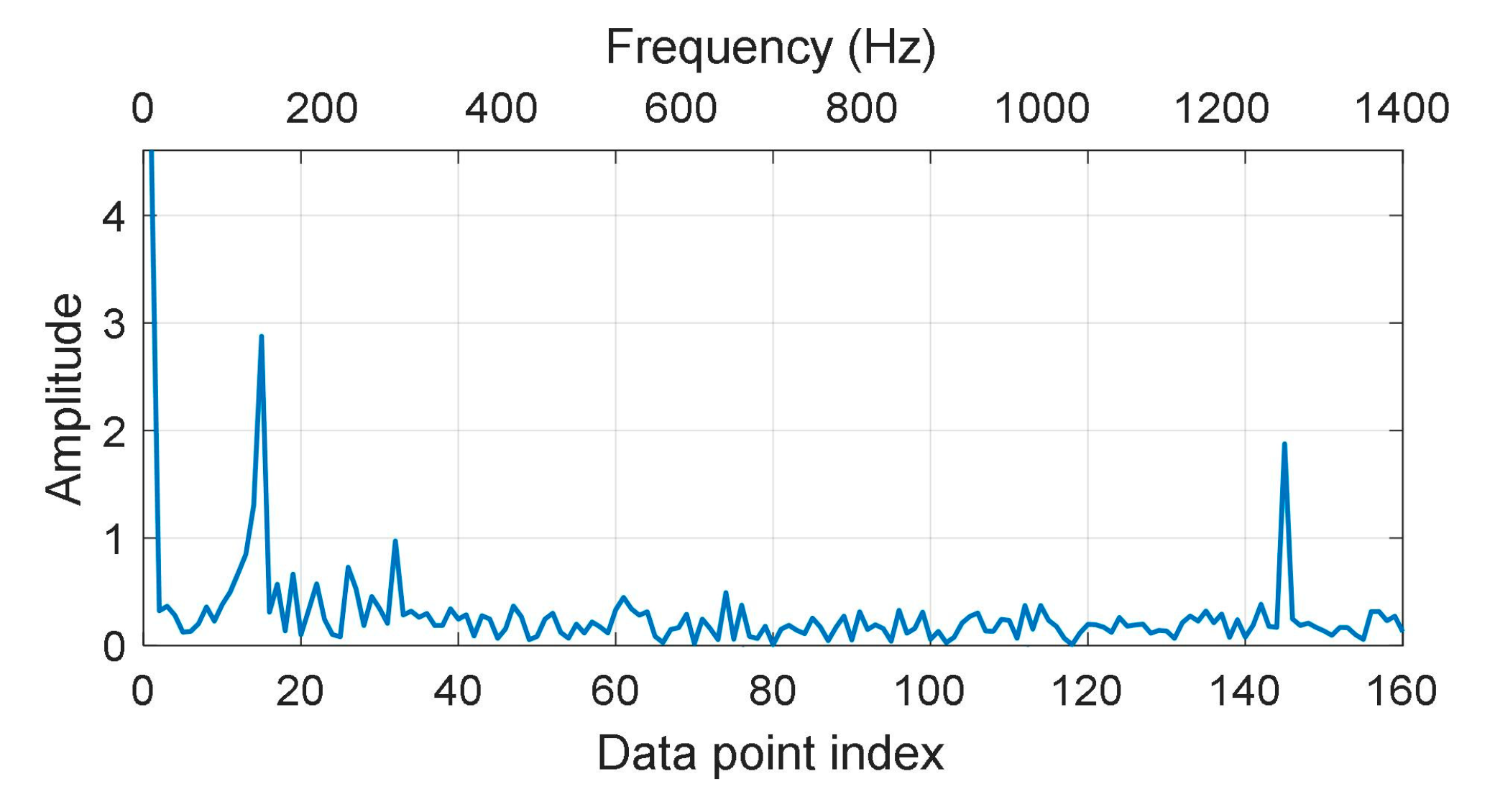
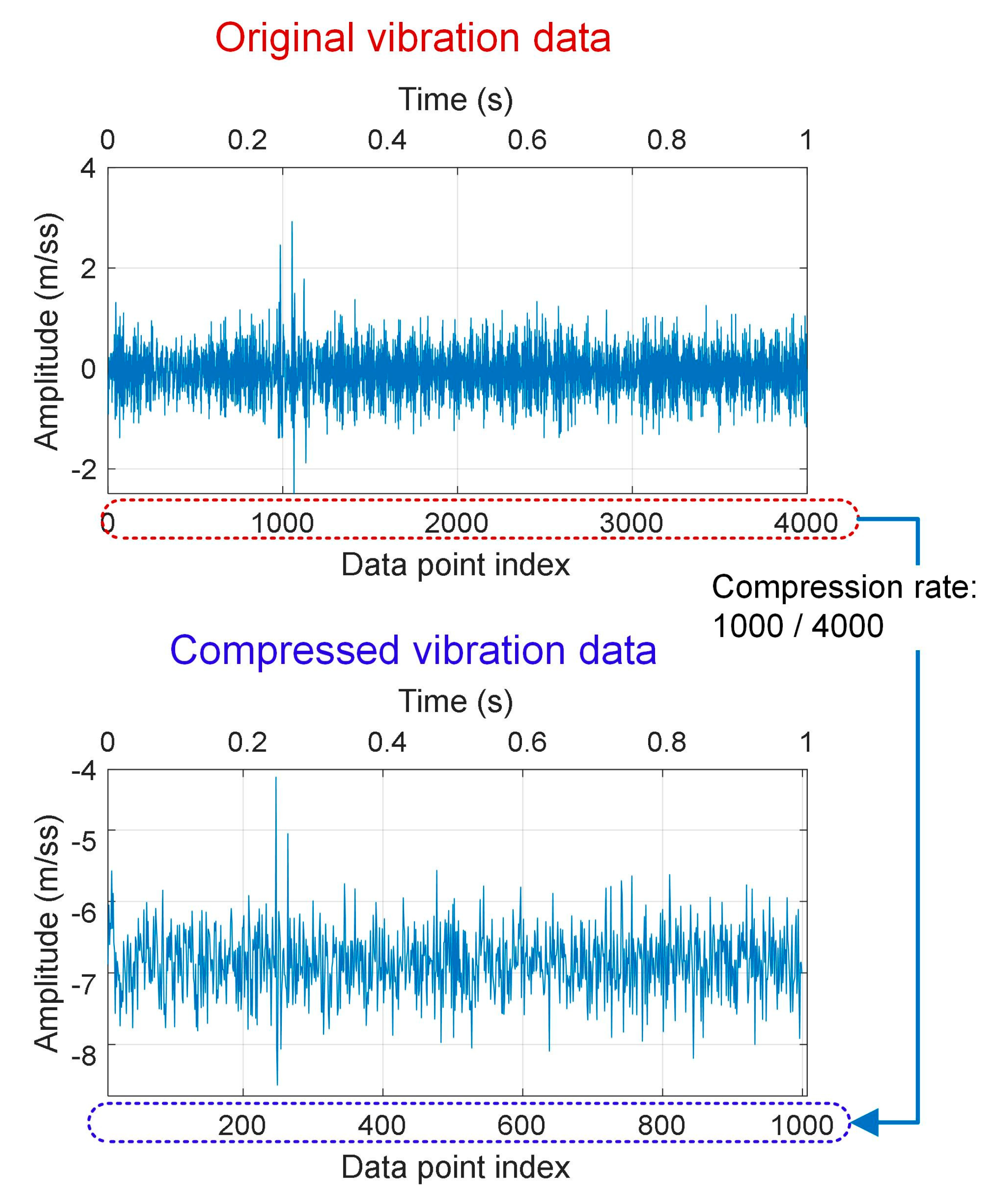
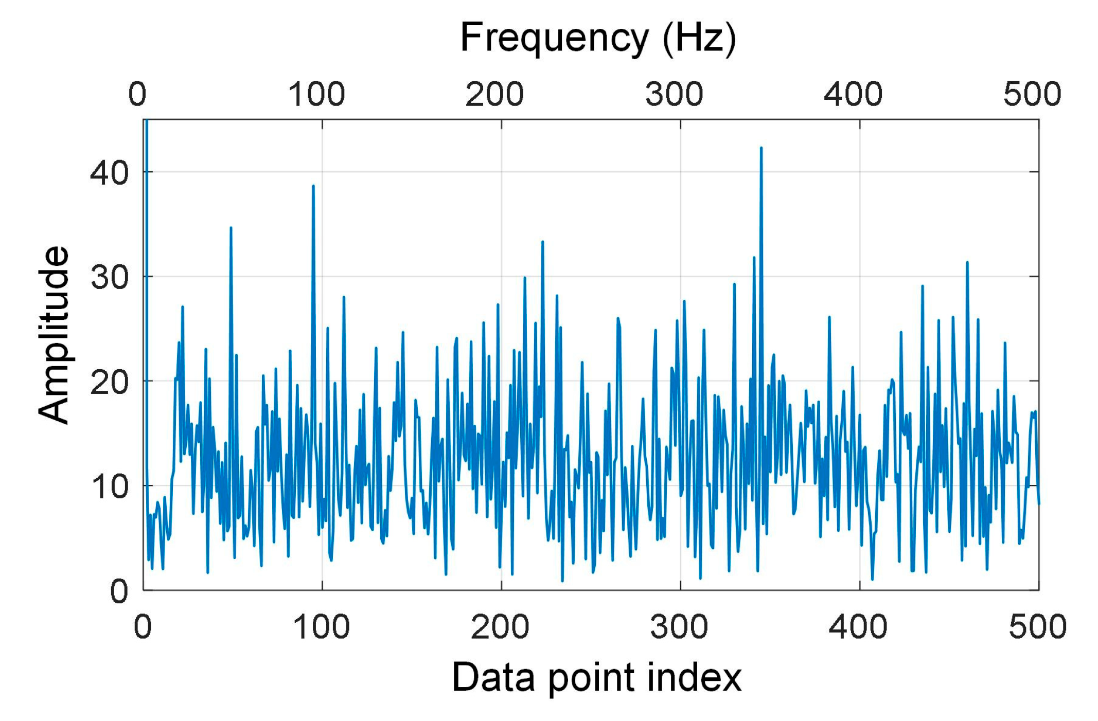
2.2. Time-Domain Compression and Time-Frequency Transform

Generally speaking, to ensure the independence of the resamples according to the measurement matrix for the original vibration signal x , a random matrix is always selected as the suitable measurement matrix. However, in this study, the frequency spectrum will later feature in the fault diagnosis, while the random measurement matrix destroys the frequency characteristics of the vibration signals: thus, a random matrix cannot be used as the measurement matrix directly.
To solve the above problem, in this study, a hybrid measurement Φ T is designed for time-domain vibration signal compression. The measurement matrix Φ T is composed of two matrices: diagonal matrix Φ T D and random matrix Φ T R . The former, Φ T D , is used to retain the frequency characteristics of the original vibration signal, and the latter, Φ T R , is utilized to ensure the independence of data resamples [17].
Suppose the original vibration signal is x N × 1 , the compressed signal is y M × 1 , and N is the integer multiple of M ; suppose also that:
N / M = c
Here, c is an integer. The diagonal matrix is then constructed as:
Φ T D = ( 1 1 1 c 0 0 0 c 0 0 0 c 0 0 0 c 1 1 1 c 0 0 0 c 0 0 0 c 0 0 0 c 1 1 1 c ) M × N
Based on measurement matrix Φ T D , the adjacent values of x are summed: in essence, it is a data down-sampling operation. Thus, the frequency characteristics of the vibration signal is retained. Φ T R is a random matrix, and its size is also M × N . Therefore, the hybrid measurement matrix is expressed as:
Φ T = Φ T D + α Φ T R
where α is the coefficient of the random matrix.
Next, the vibration signals acquired from different vibration sensors are compressed as:
y M × 1 = Φ T , M × N x N × 1
Given that two arbitrary rows of Φ T are uncorrelated, the inner production between each row of Φ T and x can be considered as an independent resample for the original signal, and all of the resamples are non-redundant.
Note that the 1st stage compression in Equation (9) is conducted in the time-domain, and the compressed data will be reconstructed for enhanced fault diagnosis or professional analysis. The reconstruction is realized based on Equations (4) and (5), and the key issue of data reconstruction is the calculation of sparse vector α ^ . Generally speaking, the nonzero elements in α ^ are obtained one-by-one based on a greedy algorithm. As described in Equation (1), the sparse vector contains k nonzero elements: to obtain all these k nonzero elements based on Equation (9), the compressed signal y should at least contain k elements. In other words, to achieve the reconstruction, the length of the 1st stage compressed M must satisfy:
M k
Meanwhile, k is determined by the characteristics of the vibration signal, and the selection of dictionary matrix Ψ for signal reconstruction in Equation (1). For vibration signals, either a discrete Fourier transform (DFT) matrix or a discrete cosine transform (DCT) matrix is always selected as the dictionary matrix. If DFT is employed as the dictionary matrix, the number of nonzero elements is that in the frequency spectrum of the vibration signal.
Based on the above analysis, to ensure the accurate reconstruction from the compressed vibration signal, the compression rate C R 1 in the 1st stage should satisfy:
C R 1 = 1 / c 1 k / N
According to our review for previous studies about the vibration signal compression and reconstruction based on compressed sensing, the compression rate of vibration signal ranges from 0.21 to 0.75.
Subsequently, the frequency spectrum of compressed signal y ( i ) , i = 1 , 2 , , M is obtained. Suppose the frequency spectrum is y f ( k 1 ) , k 1 = 0 , 1 , , M 1 , then:
y f ( k 1 ) = | 0 M 1 y ( i ) e j 2 π M k 1 i |
Considering the sampling points in y ( i ) are real numbers, then:
y f ( k 1 ) = | 0 M 1 y ( i ) ( cos 2 π k 1 i M j sin 2 π k 1 i M ) |
The frequency spectrum is symmetrical, and only half of the spectrum is therefore effective. Thus, supposing M is an even number, and M = 2 M 1 , we take the y f ( k 1 ) , k 1 = 1 , 2 , , M 1 as the effective frequency spectrum.

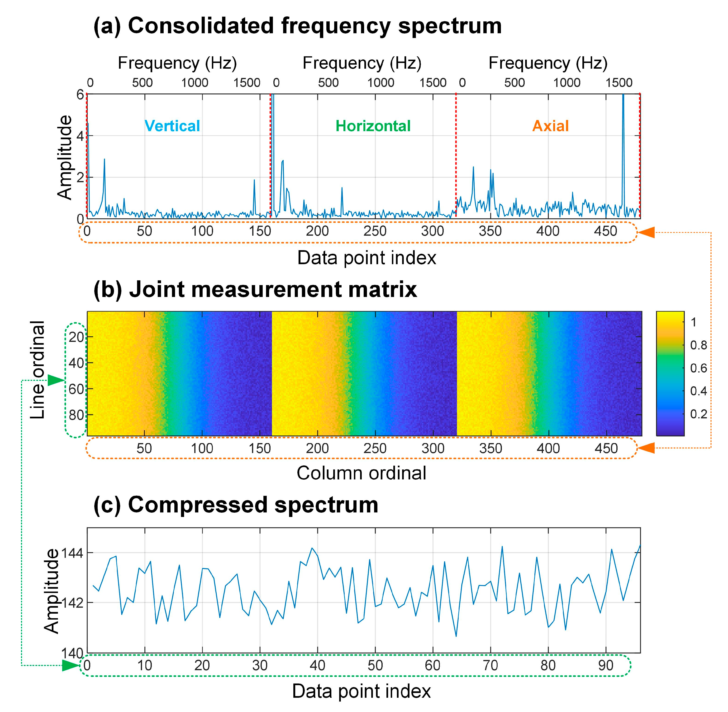
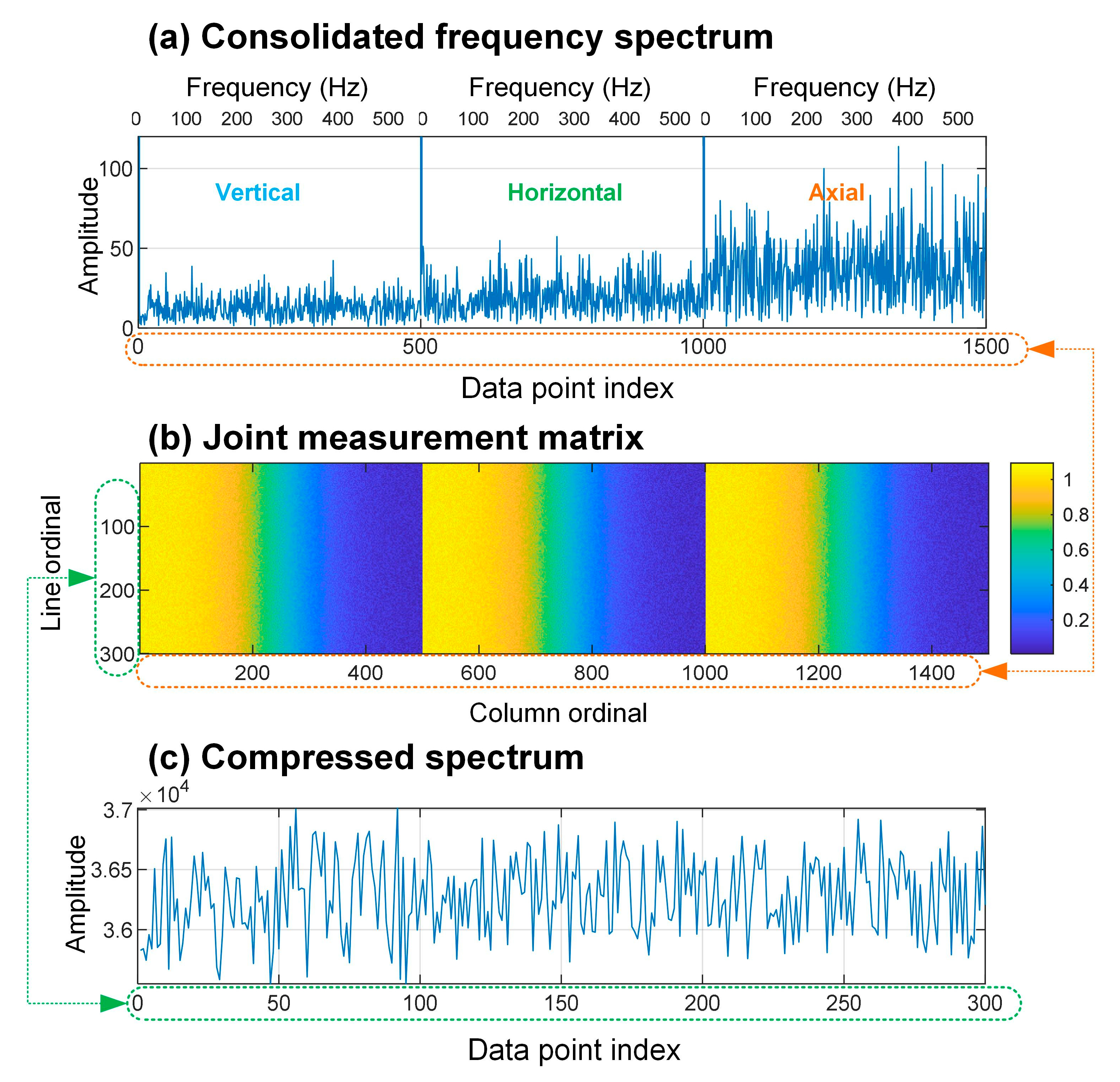
2.3. Frequency-Domain Compression and Fusion

In general, for rotating machinery, the fundamental frequency and the characteristic frequencies of faults are distributed in low and medium frequency bands, while the components in the high frequency band are always noises. Therefore, a joint measurement matrix Φ F is constructed for noise reduction, and the multi-direction frequency spectra fusion is carried out at this stage.
Suppose the effective frequency spectra of compressed vibration signals collected from different channels are y f V ( k 1 ) , y f H ( k 1 ) , and y f A ( k 1 ) , k 1 = 1 , 2 , , M 1 , and all of these spectra are expressed as column vectors; then, we consolidate these vectors as a new column vector ξ :
ξ = y f F ( k 2 ) = ( y f V ( k 1 ) T y f H ( k 1 ) T y f A ( k 1 ) T ) T , k 2 = 1 , 2 , , 3 M 1
Since data fusion improves the performance of fault diagnosis [18], a joint measurement matrix Φ F is constructed for the compression and fusion of the vector ξ , and Φ F is composed of low-pass matrix Φ F L and random matrix Φ F R :
Φ F = Φ F L + β Φ F R
where β is the coefficient of random matrix.
Based on the frequency spectrum analysis, the low-pass matrix Φ F L is generated from Equation (16) (shown in Figure 2):
y L ( t ) = 1 1 1 + e t , t ( 5 , 5 ]
Next, we fetch M 1 data points from y L with equivalent interval sampling, and these data points constitute a row vector ϕ L = y L ( k 1 ) , k 1 = 1 , 2 , , M 1 . The low-pass matrix is generated by repeating the vector ϕ L :
Φ F L = ( ϕ L ϕ L ϕ L ϕ L ϕ L ϕ L ϕ L ϕ L ϕ L ) M 2 × 3 M 1
Here, M 2 is the length of the compressed spectrum.
The size of the random matrix Φ F R is also M 2 × 3 M 1 . Based on Equation (15), the joint measurement matrix Φ F M 2 × 3 M 1 is obtained. Finally, the frequency spectra are compressed and fused using the constructed joint measurement matrix Φ F :
ν = Φ F ξ ,   ν M 2 × 1 , Φ F M 2 × 3 M 1 , ξ 3 M 1 × 1
In Equation (18), the inner product between any row of Φ F and ξ can be regarded as a resample for all the frequency spectra. Meanwhile, the fusion of three frequency spectra is achieved. Considering that each element of column vector ν is a weighted sum of ξ , and the weights corresponding to high-frequency components are smaller than others, the compression and fusion process is also a denoising process.
Unlike the compression in the 1st stage, the purposes here of the 2nd stage compression are data reduction, data fusion, and denoising. Because of the random component Φ F R in the measurement matrix Φ F , the M 2 resamples for the vector ξ are mutually independent. In view of the purpose of data reduction, the range of M 2 is M 2 [ λ , 3 M 1 ) ; in other words, to ensure the accuracy of fault diagnosis, the range of the compression ratio in the 2nd stage is:
C R 2 = M 2 / 3 M 1 [ λ / 3 M 1 , 1 )
To find out the relationship between the fault diagnosis accuracy and the compression ratio in the 2nd stage C R 2 , we carried out several fault diagnosis tests on the basis of different datasets, including the datasets employed in this study, the bearing vibration data from Paderborn University (PDBU) [19], and the widely-used bearing monitoring dataset from Case Western Reserve University (CWRU). To better demonstrate the relationship, the relative accuracy R A is employed here, which is calculated as follows:
R A = A i / M a x ( A i ) , i = 1 , 2 , , 12
where A i is the fault diagnosis accuracy of the i th test based on each dataset. For all the four datasets, 12 tests were carried out, and the relationship between C R 2 and R A is shown in Figure 3. As these tests reveal, the compression ratio in the 2nd stage should be equal to or greater than 0.2.
In many fault diagnosis methods based on compressed sensing, after the 1st stage data compression in the time-domain, the compressed data are directly used for feature extraction and fault diagnosis. Unlike these methods, in this study, the 2nd stage compression in the frequency-domain is implemented after the 1st stage compression. The reasons for the 2nd stage compression are explained as follows.
(1) After the 1st stage compression in the time-domain, many advanced feature extraction techniques are still required. However, some of these advanced feature extraction algorithms are difficult to run directly based on edge computing platform, whereas FFT is a fundamental operation for nearly all computational platforms—including embedded systems which are more practical for on-site fault diagnosis. (2) In conventional compressed sensing-based fault diagnosis, a random matrix is always employed as the measurement matrix, which destroys the frequency characteristics of the compressed signal. Fortunately, in this study, on the basis of the proposed hybrid measurement matrix in Equation (8), the frequency characteristics of the compressed signal are retained during the 1st stage compression, which makes the time-frequency transform possible. (3) For vibration signals, the high frequency components are always contaminated by noises. In this study, for the frequency spectra, by using the proposed joint measurement matrix in Equation (15), the high-frequency noises are suppressed during the 2nd stage compression. (4) For triaxial vibration signals, the 2nd stage compression in the frequency-domain further reduces the size of data during the spectrum fusion, thereby improving the computational efficiency.
In the remainder of this study, the compressed frequency spectrum ν will be employed as the feature vector of fault diagnosis.

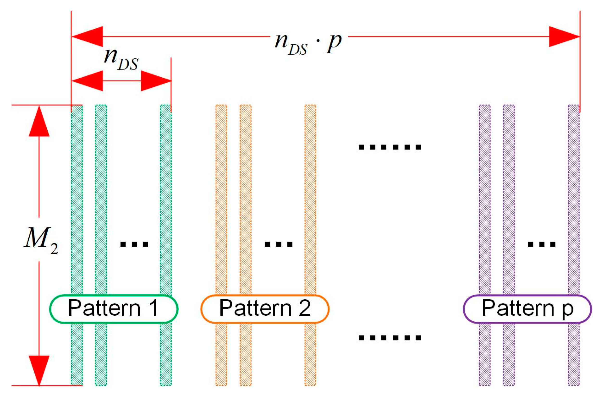
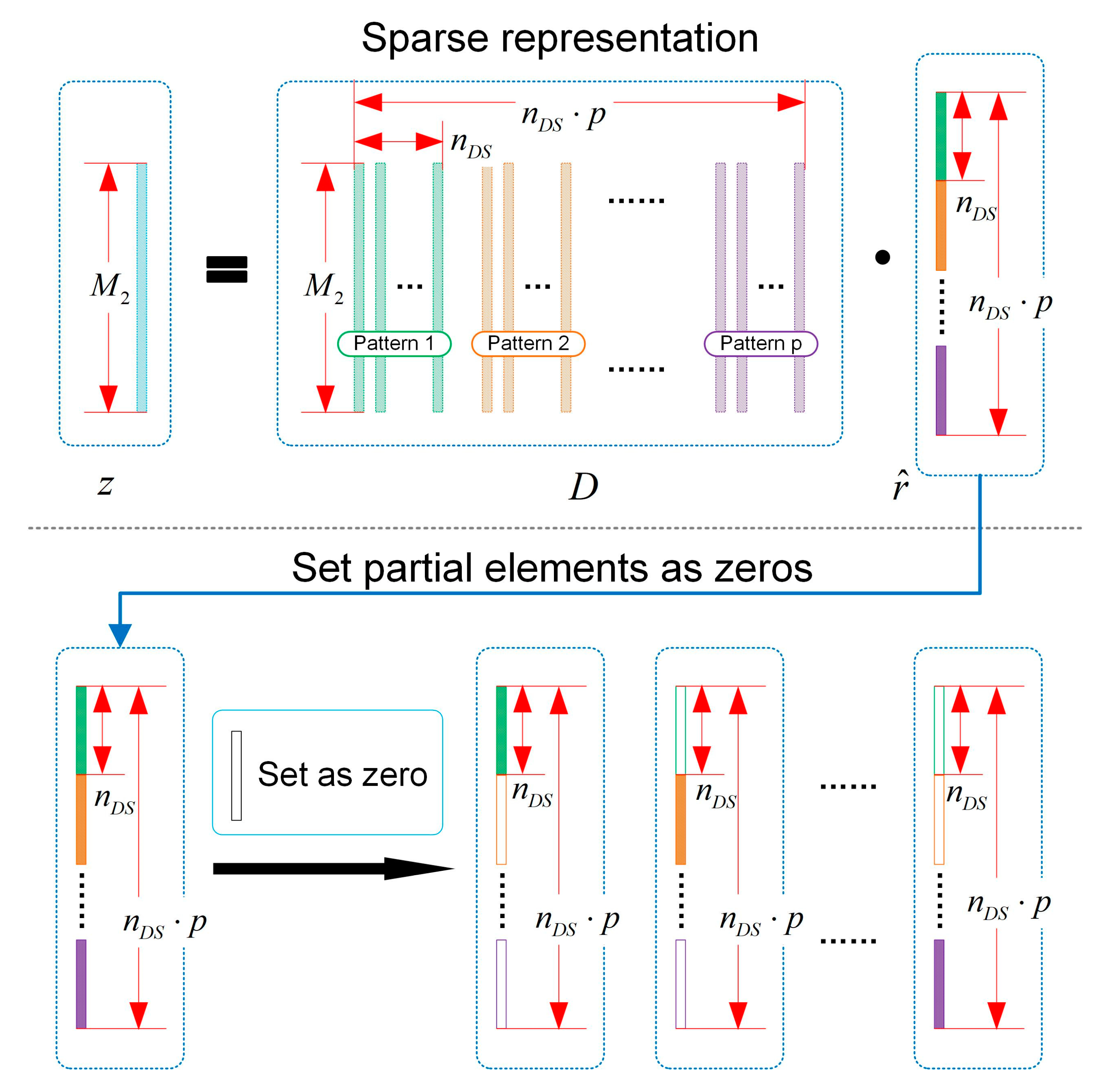
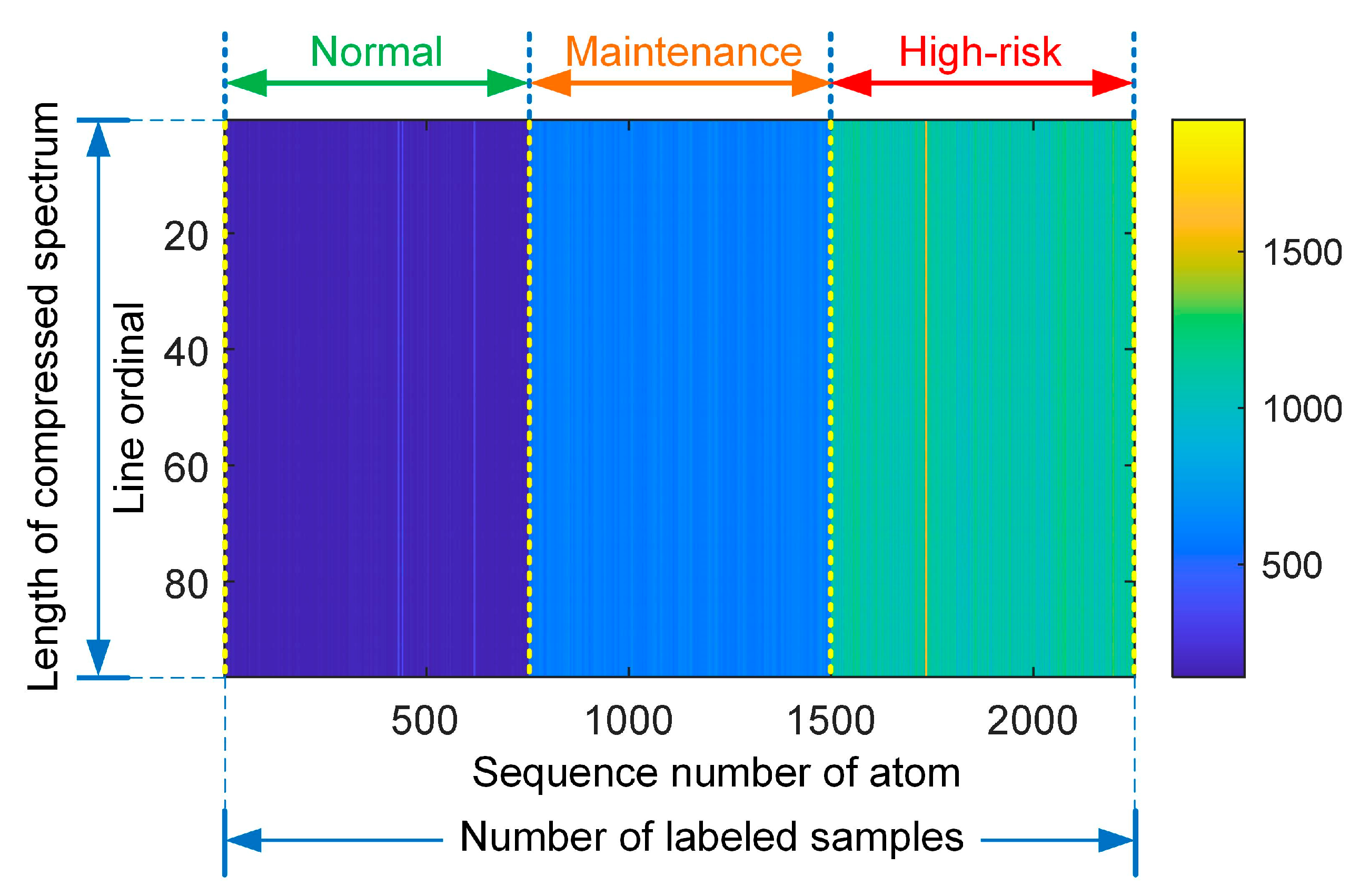
2.4. Sparse-Representation-Based Classification and Fault Diagnosis

Based on the SRC [20], the redundant dictionary matrix is constructed using the compressed frequency spectra [21]. Suppose we have p patterns, and the number of labeled samples in each pattern is n D S : then, the dictionary matrix can be shown in Figure 4:
D = ( ν 1 ν 2 ν n D S p )
Suppose the compressed frequency spectrum of testing sample is z , and its size is M 2 × 1 , the same as the size of the labeled samples in D : then, z is sparsely represented by D using the following greedy algorithm:
z M 2 × 1 = D M 2 × n D S p r ^ n D S p × 1
In Equation (22), r ^ is the estimated sparse vector, as shown in Figure 5.
The classifier is composed of sparse representation and reconstruction evaluation. In sparse representation, the compressed frequency spectrum ν obtained from Equation (18) is employed as data samples. Here, z is the testing data sample, the pattern of z is unknown and yet to be determined, and D is the dictionary matrix composed of training data, the patterns of which are known. Thus, the data samples in the dictionary matrix D are labeled samples, as shown in Figure 4 and Figure 5. Based on Equation (22), the underlying principle of fault diagnosis is that the testing sample z can be represented by the linear combination of the atoms (the labeled samples with different patterns) in the dictionary D . However, by using the atoms whose pattern are the same as the testing sample z , the number of atoms selected for representation can be minimized, because of the feature similarity. Thus, the classification problem is regarded as an optimization problem, and the object function is:
r ^ = arg min r : z = D r r 0
During the sparse representation, based on the sparse vector, the loss function is:
L = z D r
The classifier is optimized according to the proposed batch matching pursuit (BMP) algorithm, and the key procedure of the algorithm is solving a least squares problem, as expressed in the non-zero elements calculation of BMP procedures. Since the number of iterations of the algorithm is predetermined, the atoms which are most similar to the testing sample z will be selected. In fact, nonzero elements in the obtained sparse vector r ^ is determined by the weights of the linear combination, and the position indices are the sequence number of the selected atoms. Since the arrangement of labelled samples is predetermined, the pattern of the testing sample can be recognized based on the reconstruction evaluation.
To reduce the computational burden, in this study, we propose a BMP algorithm, where more than one nonzero elements are obtained in each iteration. Compared to the one-by-one principle in a traditional OMP algorithm, the calculation efficiency is improved significantly. The procedures of the proposed algorithm are listed as follows (Algorithm 1):
Algorithm 1
Algorithm input:
Redundant dictionary: D M 2 × n D S p
Compressed frequency spectrum: z M 2 × 1
Number of (fault) patterns: p
Iteration times: n I t e r
Number of support vectors contained in each iteration: n S V
Algorithm output:
Estimated sparse vector: r ^ n D S p × 1
Variables in the algorithm:
Counter of iteration: t i m e s = 1 , 2 , , n I t e r
Cosine distance between any two vectors: d cos
Indices of nonzero elements in r ^ : r ^ P o s   1 × n S V n I t e r
Nonzero elements in sparse vector: r ^ E l e m e n t   1 × n S V n I t e r
Selected support vector set for z : M S V   M 2 × n S V n I t e r
Vector of residue: R e s
Algorithm procedures:
Parameters initialization
Counter of iteration: t i m e s = 1
Sparse vector: r ^ 0 = ( 0 0 0 ) T n D S p × 1
Initial indices of nonzero elements in r ^ : r ^ P o s , 0 = [   ]
Initial vector of residue: R e s 0 = z
b. Spare vector calculation
Calculate the cosine distances between the vector of residue and each atom in the redundant dictionary:
d cos , c o l = ( ν c o l T R e s t i m e s 1 ) / ( ν c o l R e s t i m e s 1 )
ν c o l is the c o l th column vector of D , and c o l = 1 , 2 , , n D S p .
Selecting n S V maximum values from d cos , the position indices of these maximum n S V values are:
r ^ P o s , t i m e s   ,   1 × n S V = ( c o l 1 , c o l 2 , , c o l n S V )
Consequently, the obtained position indices in the iteration are merged into the existing position indices:
r ^ P o s = r ^ P o s r ^ P o s , t i m e s
Next, based on r ^ P o s , a batch of support vectors is selected from the redundant dictionary, and these support vectors contribute most in the reconstruction:
M S V , t i m e s = D r ^ P o s = D ( : , r ^ P o s )
After that, the selected atoms in the redundant dictionary are replaced by null vectors:
D ( : , r ^ P o s , t i m e s ) = 0
By using M S V , t i m e s , the nonzero elements in r ^ E l e m e n t , t i m e s are calculated based on the least-square method:
r ^ E l e m e n t , t i m e s = ( M S V , t i m e s T M S V , t i m e s ) 1 M S V , t i m e s T z
After this process, the new residual vector R e s t i m e s is calculated:
R e s t i m e s = z M S V , t i m e s r ^ E l e m e n t , t i m e s
c. Iteration
The procedures in sparse vector calculation are repeatedly executed for n I t e r times, and n S V n I t e r nonzero elements in the sparse vector are obtained.
Finally, these nonzero elements are filled into the sparse vector in accordance with the vector of indices r ^ P o s :
r ^ n D S p × 1 :   r ^ r ^ P o s = r ^ ( r ^ P o s ) = r ^ E l e m e n t
Compared to the traditional OMP algorithm [22], the number of iterations of BMP is 1 / n S V times of OMP, which reduces the computational burden significantly. Thus, for the edge computing platform and on-site fault diagnosis, the BMP algorithm provides a more efficient solution.
After sparse representation, reconstruction evaluation is conducted to determine the pattern of samples tested. Since the atoms or the labeled samples in the dictionary D are grouped by patterns, and each column vector in matrix D corresponds to a single element in the sparse vector r ^ , the values and distributions of nonzero values in r ^ indicate the pattern of the testing sample. Thus, the estimated sparse vector r ^ is divided into p isometric parts, each part containing n D S elements based on retention of partial elements (other elements being set as zeros), p partial sparse vectors are derived from r ^ , and these partial sparse vectors are denoted r ^ 1 , r ^ 2 , …, r ^ p respectively, as shown in Figure 5.
Next, we reconstruct the compressed frequency spectrum of testing sample z by using the partial sparse vectors r ^ u , u = 1 , 2 , , p , respectively:
z ^ u = D r ^ u , u = 1 , 2 , , p
By comparing z and z ^ u , the reconstruction error can be obtained:
E r r u = z z ^ u / z   ( u = 1 , 2 , , p )
Based on sparse representation and compressed sensing, the partial sparse vector—composed of the elements corresponding to the targeted atoms in the dictionary matrix—reconstructs z better than other vectors. Thus, the subscript of the minimum E r r u is the pattern to be determined [10]:
Pattern = u     s . t . min ( E r r u )   u = 1 , 2 , , p

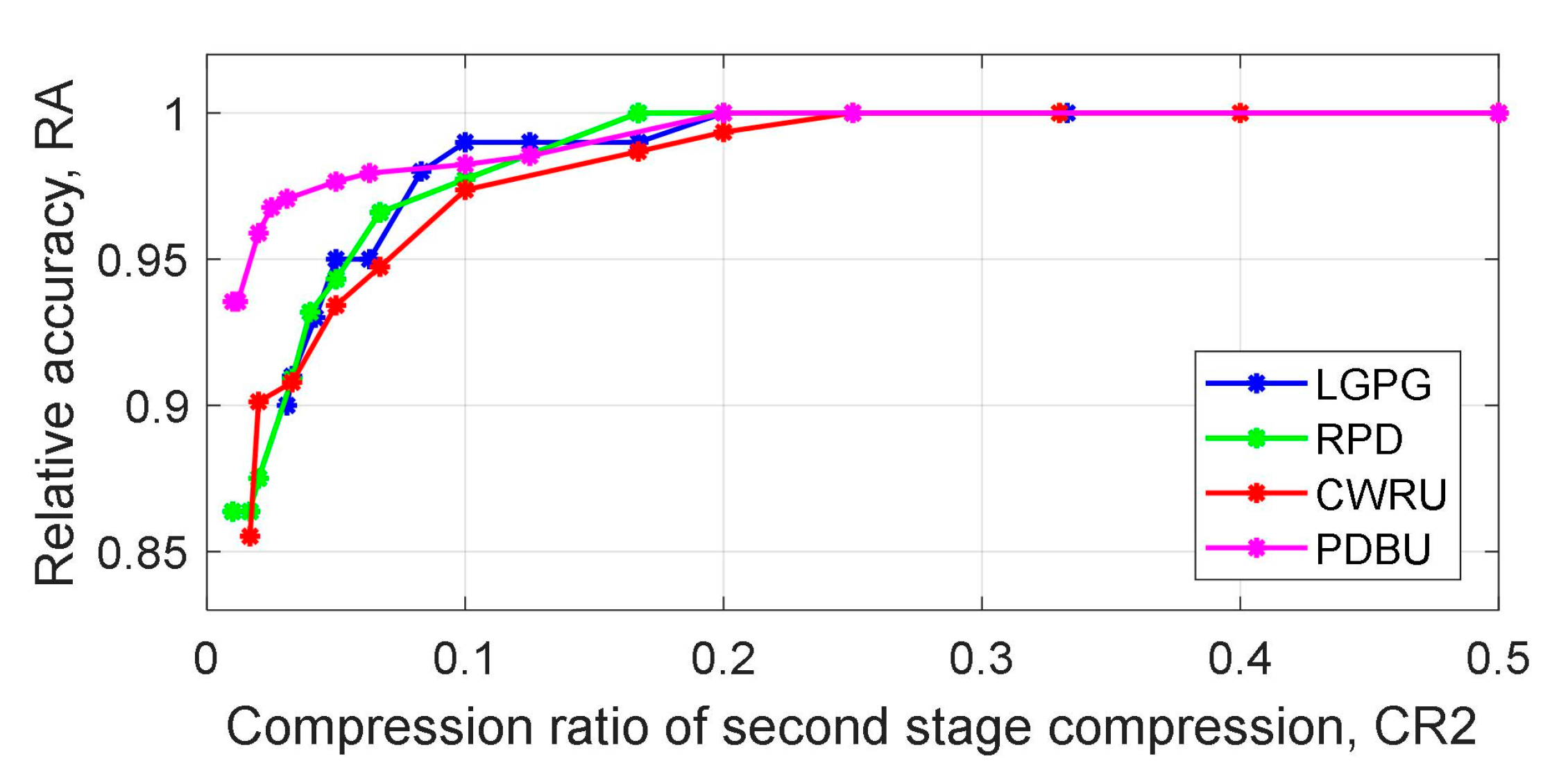
3. Efficiency Analysis

In this section, the efficiency of the proposed method is analyzed from two perspectives: the data size analysis, and the key algorithm efficiency analysis. The analyses are based on triaxial vibration signals.

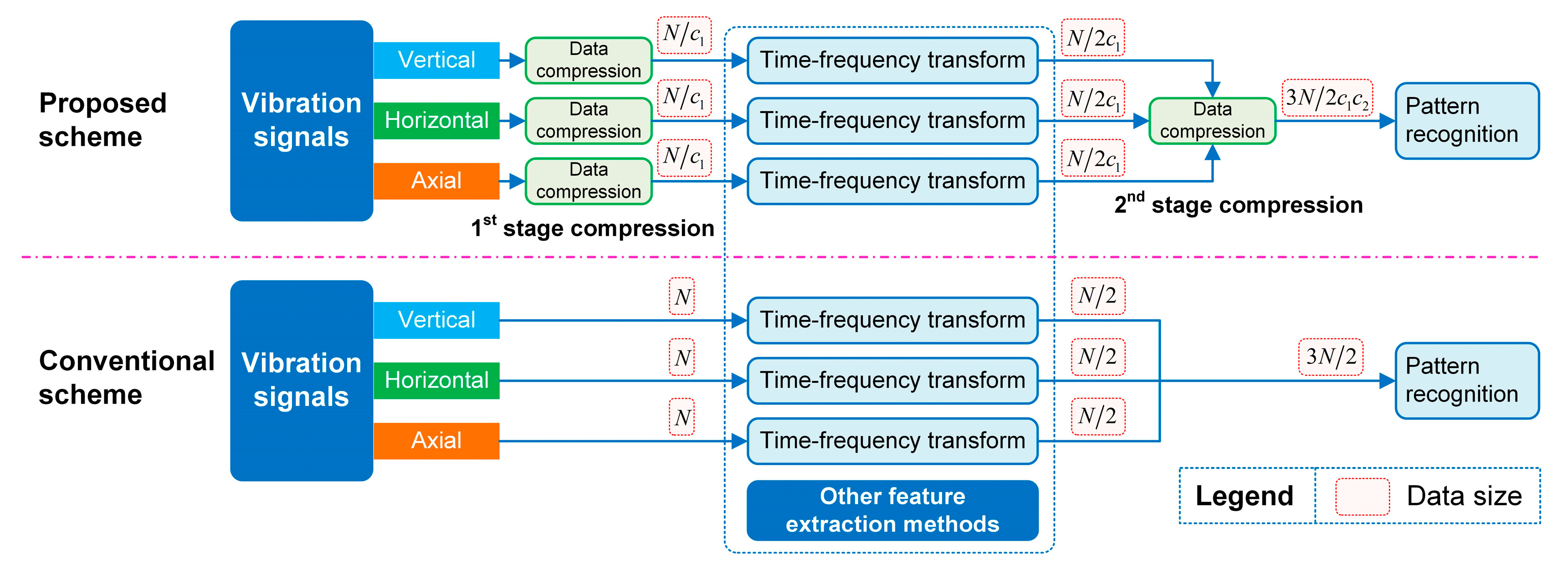
3.1. Data Size Analysis

Generally, the classical fault diagnosis scheme is composed of feature extraction and pattern recognition. To ensure the accuracy of fault diagnosis, time-domain features, frequency-domain features, and time-frequency domain features are always extracted from the triaxial vibration signals. Since frequency-domain analysis is critical for fault diagnosis based on vibration signals, here, we compare the data size of the proposed scheme with that of the conventional scheme for time-frequency analysis based on triaxial vibration data. The data size in the fault diagnosis procedures are shown in the dash red frames of Figure 6, where c 1 is the reciprocal value of the 1st stage compression ratio, and c 2 is the reciprocal value of the 2nd stage compression ratio.
Note that the data compression is based on inner product between the measurement matrix and the original vibration signal, as shown in Equations (9) and (18). In essence, the compression is an inner product between a matrix and a vector. For the 1st stage compression, the size of the measurement matrix is M × N , and the size of the original vibration signal is N × 1 ; thus, the computational complexity of the 1st stage compression is O ( M N ) . Here, we take the Fourier transform as a benchmark: the computational complexity of the Fourier transform for the original vibration signal is O ( N N ) , which is lower than other advanced feature extraction and pattern recognition algorithms. Since N / M = c 1 , the computational complexity of the 1st stage compression is only 1 / c 1 times that of the Fourier transform. Similarly, the computational complexity of the 2nd stage compression is O ( M 2 3 M 1 ) . Thus, for feature extraction, except for the data compression, the computational burden of the proposed method is 1 / c 1 times that of the conventional method; and for pattern recognition, the ratio is 1 / c 1 c 2 .
As a rule, to ensure the accuracy of data reconstruction for professional analysis, the compression ratio of the 1st stage compression c 1 is smaller than 5. For example, in Section 4.1 of this study, the 1st stage compression ratio was c 1 = 3 , and the 2nd stage compression ratio was c 2 = 5 ; thus, for both feature extraction and pattern recognition, the computational burdens were reduced significantly.
Comparing the overall computational burden based on time consumption under the same conditions with respect to feature extraction algorithms such as time-frequency transform, wavelet package decomposition, or empirical mode decomposition, the total computational burden of the proposed method is much smaller. This conclusion is supported by the comparison of relative time consumption depicted in comparative case study.

3.2. Sparse Representation Efficiency Analysis

The key procedure of fault diagnosis is sparse representation-based classification, and from the perspective of computation burden, sparse representation consumes most of computational resources. Thus, the improvement of fault diagnosis efficiency is mainly determined by efficiency promotion of the sparse representation algorithm. In this study, the widely-used OMP algorithm is improved upon by the BMP algorithm.
In the OMP algorithm, in each iteration, only one atom is selected from the dictionary matrix. If we then need n nonzero elements in the sparse vector, n atoms are supposed to be selected from the dictionary matrix: thus, the number of iterations is n . Since n D S p vector multiplications are conducted in each iteration, the total number of vector multiplications is n D S p n .
In the BMP algorithm proposed in this study, n S V atoms are selected in each iteration. Thus, if n atoms are required, only n / n S V iterations are required, and the total number of vector multiplications is n D S p n / n S V . Therefore, the proposed BMP algorithm increases the computational efficiency for n S V times.

4. Case Study

4.1. Maintenance Level Recognition of Landfill Gas Power Generator

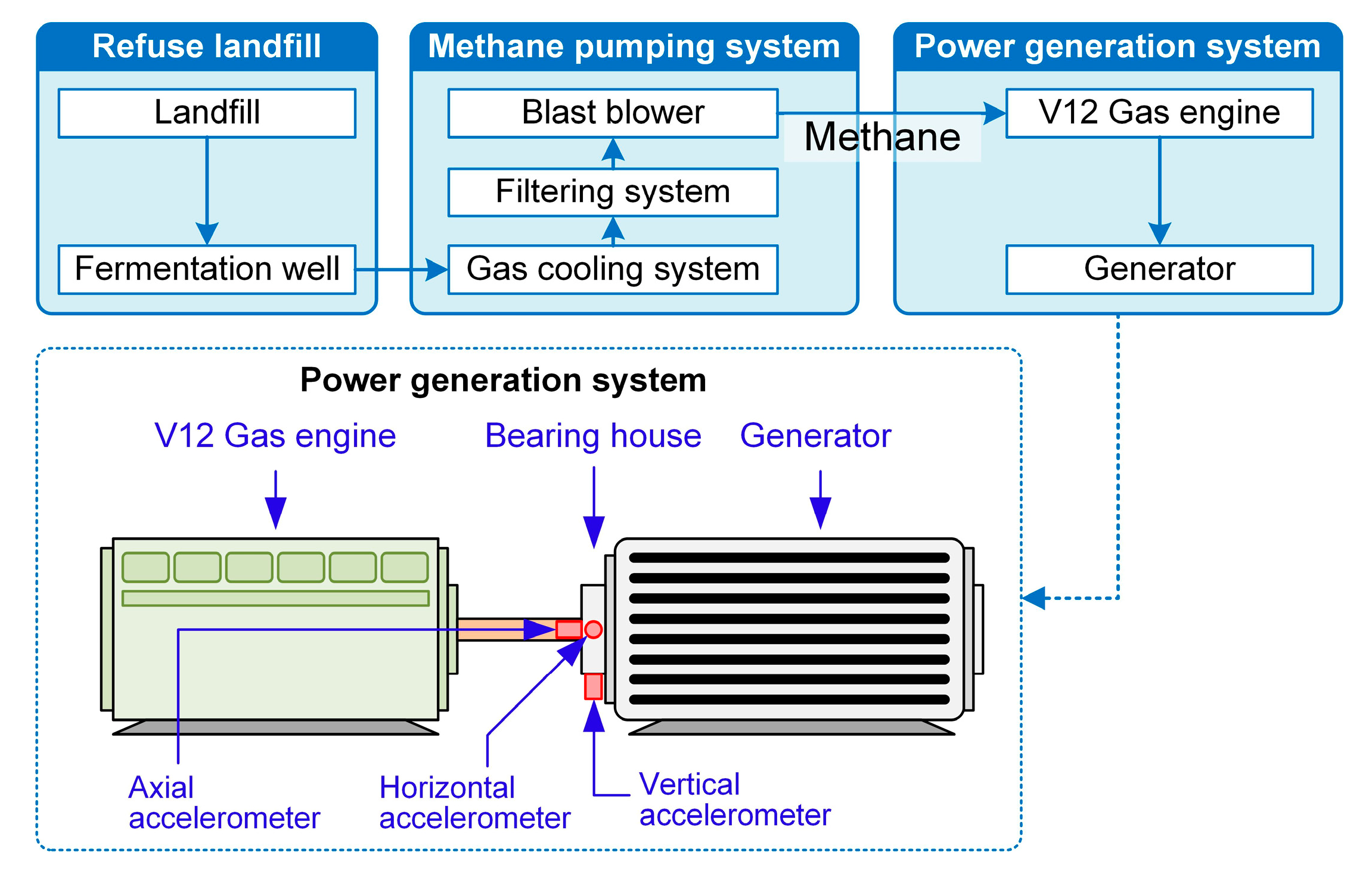
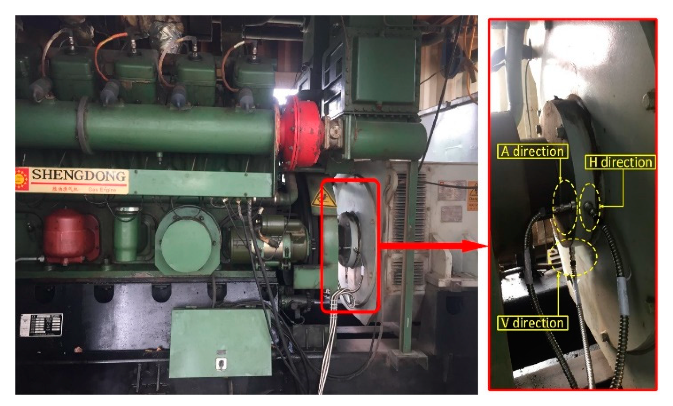
4.1.1. Engineering Background

Landfills are generally located in remote areas; thus, efficient data compression, fusion, storage and on-site maintenance level recognition are necessary. Meanwhile, for some intractable faults, such as coherent faults, professional analysis and enhanced fault diagnosis based on the original data are needed. Therefore, data reconstruction from the compressed data is also essential.
The schematic diagram of the landfill gas power generator (LGPG) case study is shown in Figure 7, and its real figure is shown in Figure 8. The LGPG is driven by a gas engine; the generator and gas engine are connected by a shaft supported by several bearings. Because of harsh conditions such as electric corrosion, the bearings are always damaged, and to prevent system breakdown, condition-based maintenance is essential. Thus, in this section, maintenance level recognition is applied to the LGPG. To ensure the safety and stability of power generation, professional vibration analysis is implemented for the LGPGs periodically by vibration analysts certified by ISO-18436, based on the vibration data acquired in the field, and maintenance recommendations are provided. In the maintenance report, the maintenance level for the rotor system of the LGPG is identified as normal, maintenance, or high-risk, according to the fault pattern or degradation condition. In the normal condition, the rotor system works well, and regular inspection is required; in the maintenance condition, more inspections and services are recommended for the system; while in the high-risk condition, spare parts should be purchased for replacement, or the LGPG should be shut down for further investigation.
Note that the type of bearings in the LGPG is 6924C3 manufactured by KOYO, and the rotational speed of the system is around 1000RPM. Vibration data were collected using three vibration sensors, mounted on the bearing house of the generator, as shown in Figure 8. Three vibration sensors were mounted: in the axial direction (A direction), horizontal direction (H direction) and vertical direction (V direction), respectively. The vibration data were acquired for 12 s every 4 h synchronously, and the sampling rate of data acquisition was 8   K S / s .

4.1.2. Data Set Description

The project lasted for nearly four months, and 30 data files were employed for maintenance pattern recognition. Since the sampling rate was 8   K S / s , and each acquisition lasted for 12 s, one data file contained 96,000 data points for each channel. Considering the rotational speed was 1000 RPM, for each channel, a rotational cycle of the shaft contained 480 data points. Vibration data collected during two rotational cycles were defined as a data sample, and the number of data points in each data sample was 960; thus, one data file can be divided into 100 data samples. The details of data samples are shown in Table 1.
Based on the maintenance manual of the LGPG, the maintenance operations can be divided as maintenance and high-risk, and the component should be replaced for high-risk conditions. Thus, the patterns to be recognized contains normal, maintenance, and high-risk, as shown in Table 2, where 750 labeled data samples were utilized to construct the dictionary matrix, while the other 250 data samples in each pattern were used for algorithm validation.

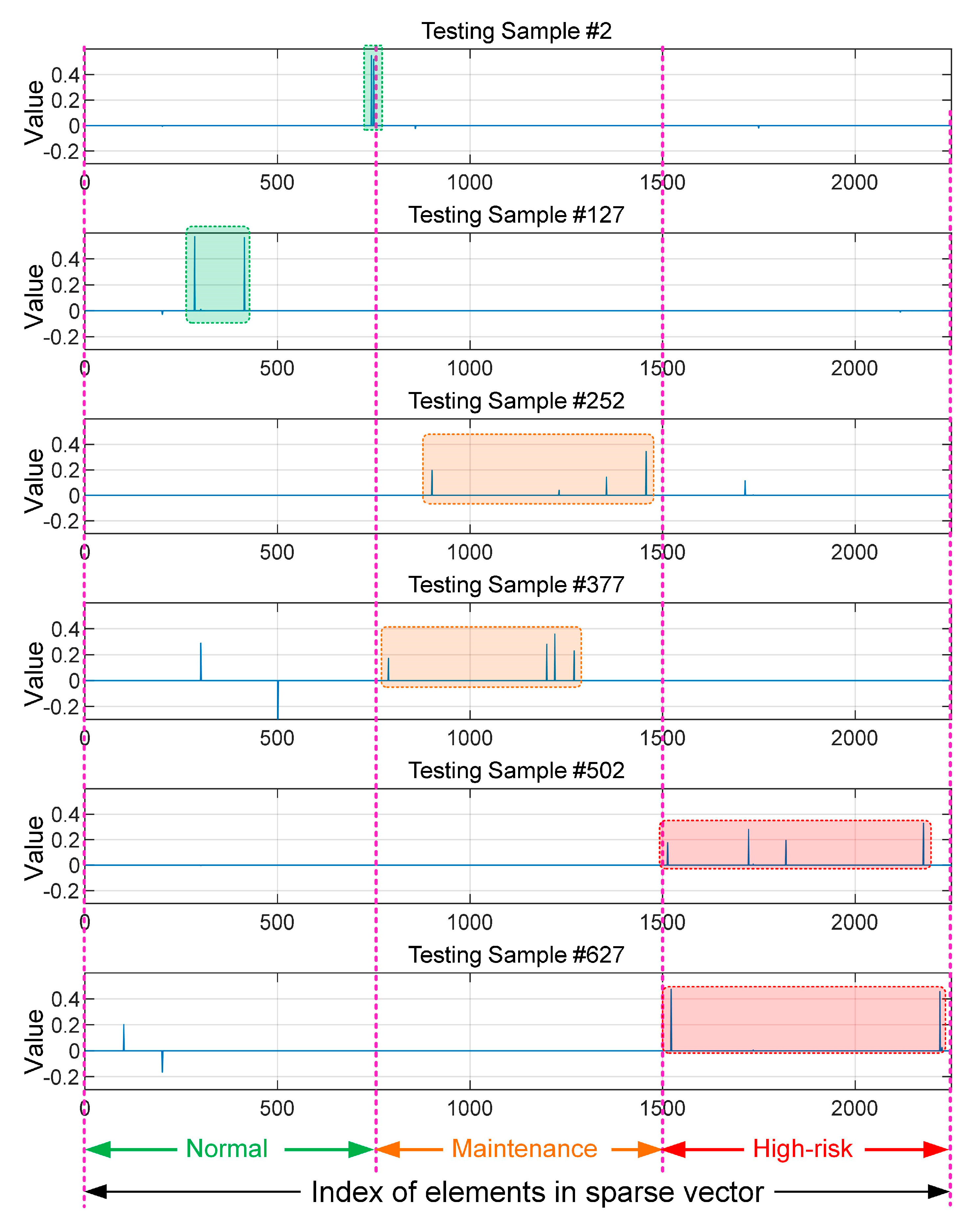
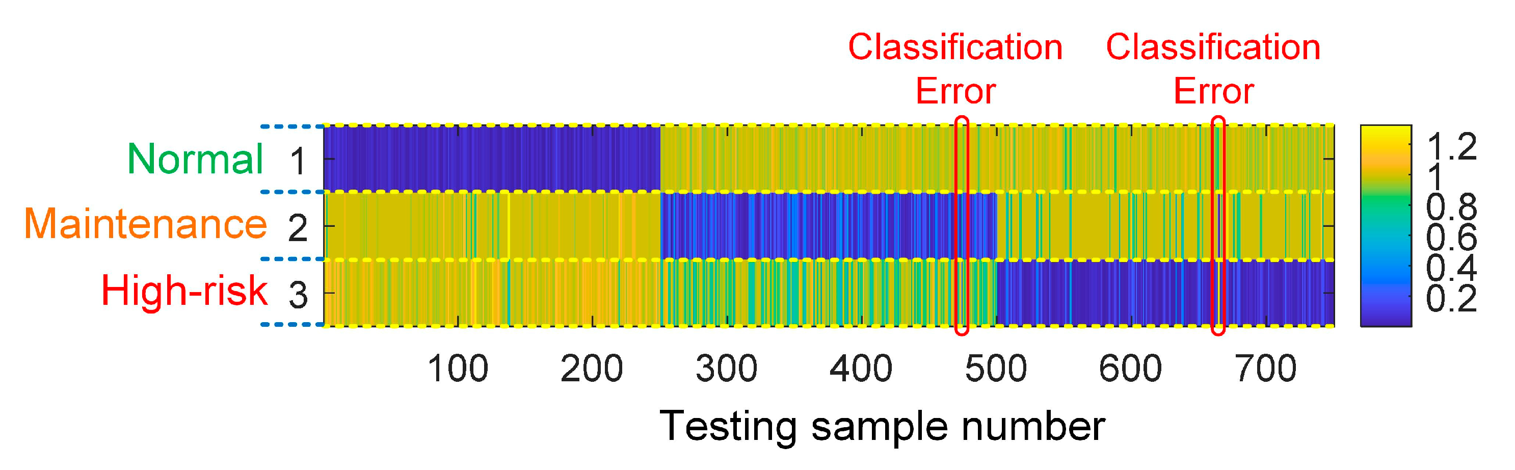
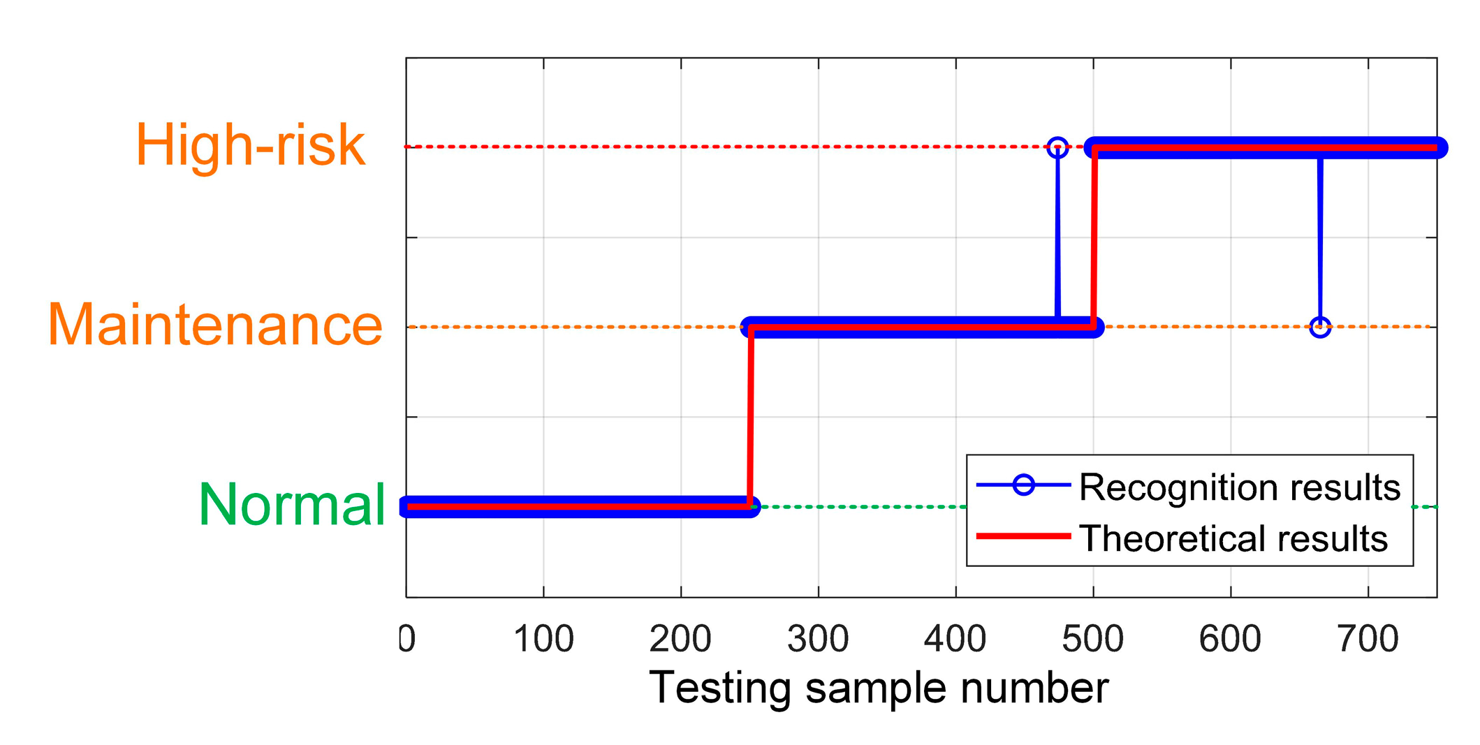
4.1.3. Data Processing and Pattern Recognition

Based on the definition of data samples, the length of the original data sample was N = 960 . In the 1st stage compression, based on compressed sensing, the length N = 960 was shortened to M = 320 , which means that three data points in the original vibration signal were compressed to one data point in the compressed vector.
The size of the diagonal matrix, random matrix, and hybrid measurement matrix were M × N = 320 × 960 , and these matrices are shown in Figure 9. Here, the coefficient of random matrix was α = 0.05 . Based on Equation (9), the length of the compressed data was 320, and the original and the compressed vibration data are shown in Figure 10. because of the compression, the number of data points was reduced, as indicated in the x-axis (data point index). As mentioned in Equation (8), the compression in the time-domain can be regarded as a data down-sampling operation. Therefore, compared with the original vibration signal, the sampling rate of the compressed vibration data was M / N = 320 / 960 times that of the original vibration data, while their time record lengths were the same, as indicated in the time axis in Figure 10. The results indicate that, based on the constructed hybrid measurement matrix, the variation of the compressed vibration signal is nearly identical to the original vibration signal, except for the signal length. Meanwhile, a part of the high-frequency component is removed.
Next, the frequency spectrum of the compressed signal was obtained based on Equation (13), as illustrated in Figure 11: the spectrum partly retains the frequency characteristics of the vibration data.
Later, in the 2nd stage compression, the spectra obtained from the vibration data in all directions were compressed and fused based on the joint measurement matrix. First, the spectra were connected in order of vertical, horizontal, and axial directions longitudinally, and the resulting length was 3 M 1 = 3 × 160 = 480 , the consolidated frequency spectrum is shown in Figure 12a. Next, the joint measurement matrix Φ F was constructed: the coefficient of random matrix in Φ F was β = 0.1 , and its size was M 2 × 3 M 1 = 96 × 480 , as shown in Figure 12b, revealing the compression rate was 96 ÷ 480 = 0.2 . Based on Equation (18), the consolidated frequency spectrum was compressed, and the spectra were fused synchronously. the resulting compressed spectrum ν is shown in Figure 12c, and its length was M 2 = 96 .
The redundant dictionary D was constructed using the compressed spectra based on Equation (21) and Figure 4, and the compressed spectra—used as atoms in the dictionary—were grouped by patterns of labeled samples, as listed in the 2nd row of Table 2. The dictionary matrix is shown in Figure 13, and its size is M 2 × n D S p = 96 × 2250 .
As shown in the 3rd row of Table 2, to validate the proposed method, for each maintenance pattern, 250 testing sample were employed. For the testing samples, based on the BMP algorithm and the constructed dictionary D shown in Figure 13, the sparse vectors were obtained. In the calculation, the number of support vectors in each iteration was n S V = 2 , and the number of iterations was n I t e r = 3 . As shown in Figure 14, for testing samples #2, #127, #152, #377, #502, and #627, the values and position indices of nonzero elements in the calculated sparse vectors indicate their patterns.
Finally, three partial sparse vectors were derived from the original sparse vector r ^ . These partial sparse vectors were employed to reconstruct the compressed spectrum respectively, and the reconstruction errors were calculated based on Equation (26). Supposing the corresponding reconstruction errors of r ^ 1 , r ^ 2 , r ^ 3 were E r r i , 1 , E r r i , 2 , E r r i , 3 , and i = 1 , 2 , , 750 was the number of testing sample, then, the reconstruction error matrix was:
E R R = [ E r r 1 , 1 E r r 2 , 1 E r r 3 , 1 E r r 750 , 1 E r r 1 , 2 E r r 2 , 2 E r r 3 , 2 E r r 750 , 2 E r r 1 , 3 E r r 2 , 3 E r r 3 , 3 E r r 750 , 3 ] 3 × 750
The reconstruction error matrix is shown in Figure 15, and two testing samples (#474 and #665) were misclassified. The pattern recognition results are shown in Figure 16: since the number of testing samples was 750, the diagnosis accuracy was 99.73%.

4.1.4. Data Reconstruction and Analysis

Another advantage of the proposed fault diagnosis scheme is that the compressed data can also be reconstructed based on compressed sensing, although the constructed signal is not identical with the original signal. In view of the low storage-consumption and the low-computational consumption, this is acceptable in engineering applications.
In this case study, the compression rate was 0.33: we therefore saved 66.67% in data storage and computational resources. In the data reconstruction, a discrete Fourier transform (DFT) matrix was employed as the dictionary matrix, and its size was 960 × 960 . A traditional OMP algorithm was then used to calculate the sparse vector [22]. Here, we take the 1st vibration signal of horizontal direction as an example. The original vibration signal and the reconstructed vibration signal are shown in Figure 17: it is noteworthy that the time record lengths of all signals in Figure 17 are identical, while the number of data points in the compressed vibration signal are much less than that of the original and reconstructed vibration signals. The results reveal that the reconstructed signal is nearly identical to the original vibration signal; thus, the enhanced fault diagnosis or professional vibration analysis can be conducted accurately based on the reconstructed signal.

4.2. Fault Diagnosis of Driving Gear in Battery Swapping System

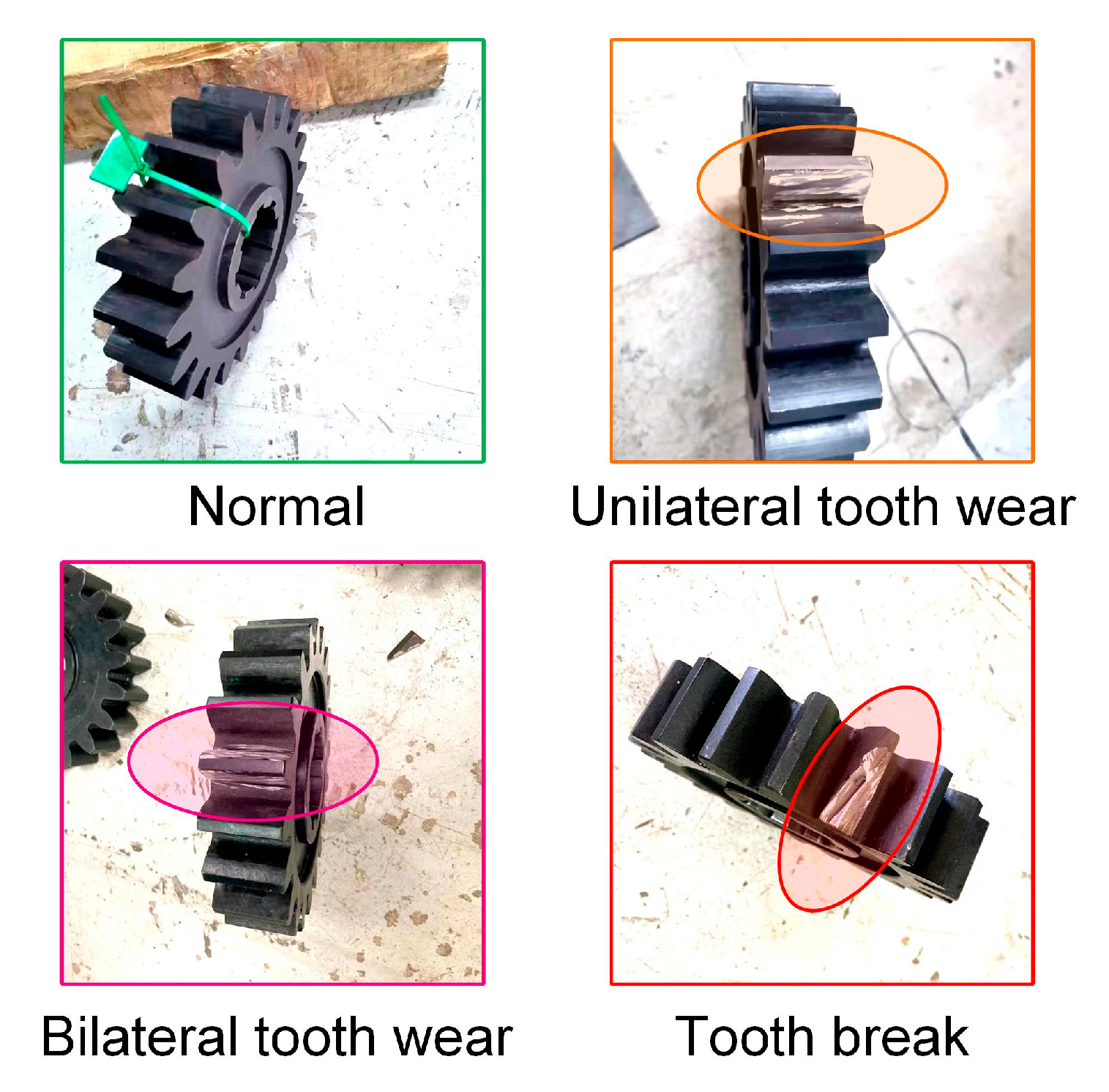
4.2.1. Engineering Background

The application of a battery swapping system (BSS) increases the efficiency of electric heavy truck (EHT) operation. However, because of the conditions of electrification, the driving gear in rack and pinion drives (RPD) of BSSs are always damaged by electric erosion, leading to gear tooth surface wear, or even causing teeth to break. To improve the efficiency of maintenance and commercial transportation, fault diagnosis for the driving gear is necessary.
As shown in Figure 18 and Figure 19, the driving gear is a key component of a BSS. For this research, in the uniform motion stage, the rotating speed was 180RPM. Vibration signals were acquired by using three vibration sensors (axial, horizontal, and vertical) and the data acquisition chassis synchronously; the vibration sensors were mounted near the driving gear, as shown in the left part of Figure 19; and the sampling rate was 4 KS/s. The uniform motion time consumption of one single-direction motion cycle was 1 s, which means that one data sample contained 4000 data points.

4.2.2. Description of Data Sets

In this case, three kinds of faults were injected to the driving gear: unilateral tooth wear (UTW), bilateral tooth wear (BTW), and tooth break (TB), as shown in Figure 20.
The data sets are described in detail in Table 3. The number of labeled samples was 60, and the features of these labeled samples were utilized to construct a dictionary matrix, while other samples were employed as testing samples. The arrangements of the dictionary matrix and testing samples are shown in Table 4.

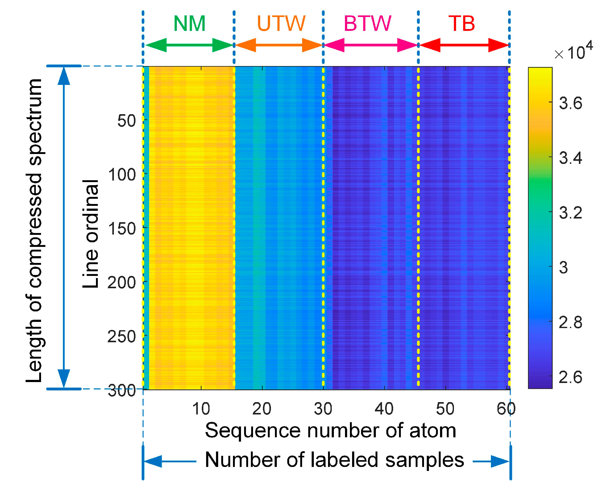
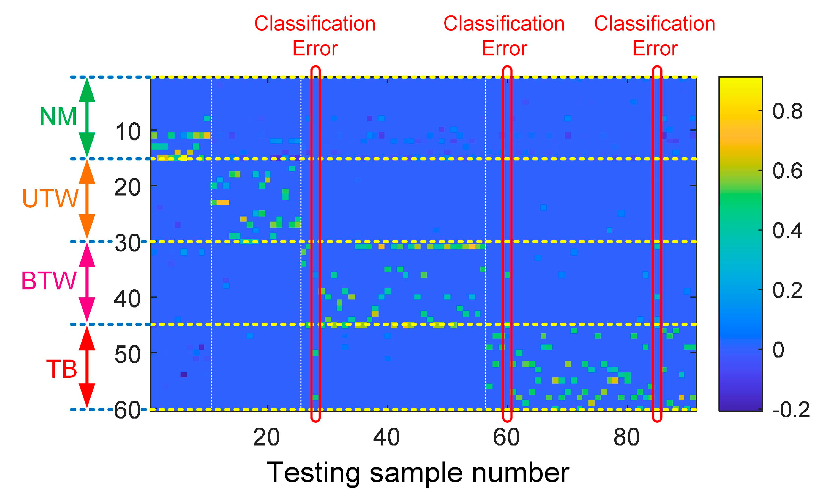
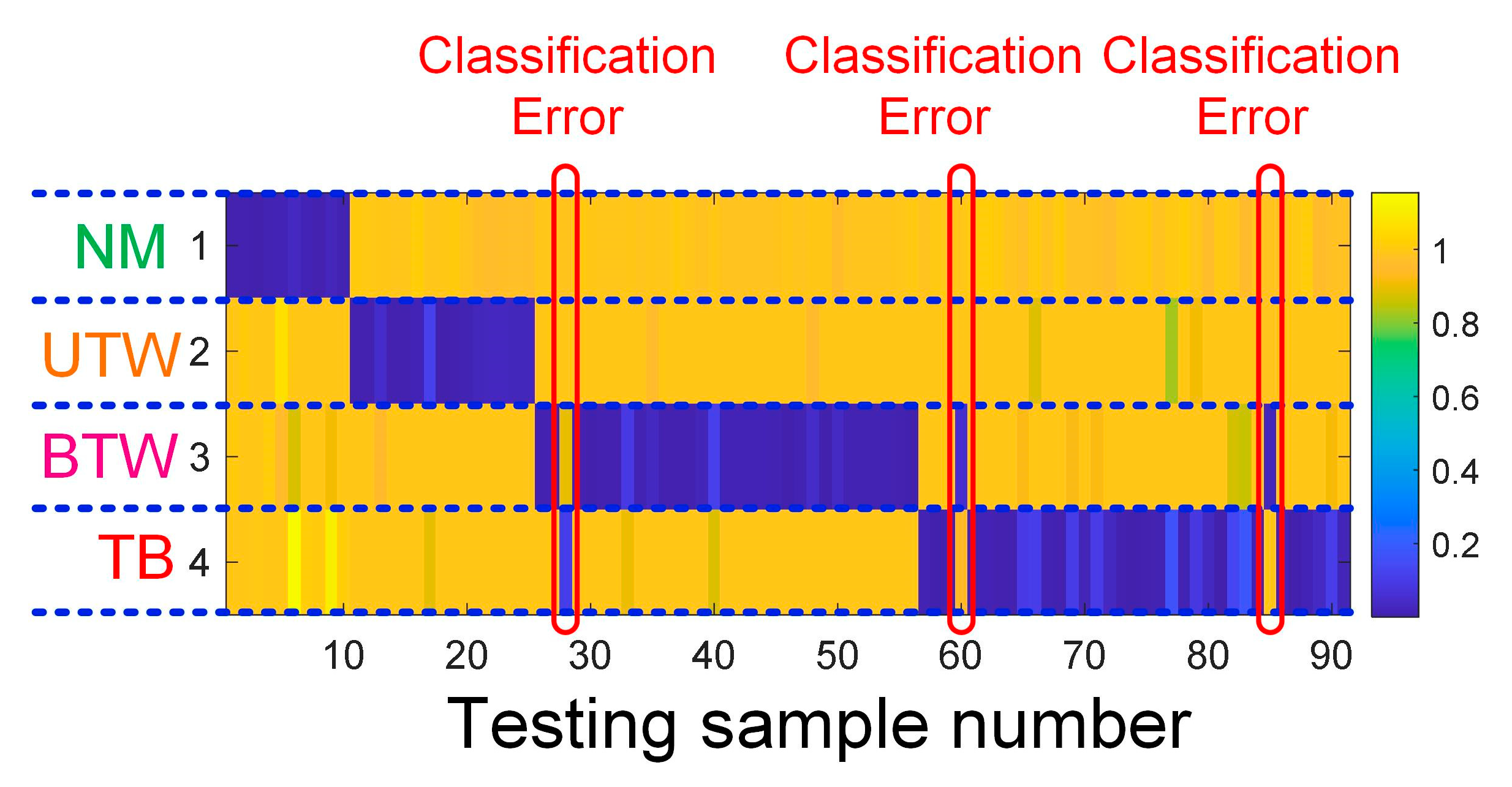
4.2.3. Data Processing and Fault Diagnosis

The length of each data sample was N = 4000 ; in other words, the size of the original vibration signal was 4000 × 1 . Here, in the time-domain compression, the compression rate was 0.25; thus, the length of the compressed vibration signal was M = 1000 , and four data points in the original vibration signal were compressed to one data point in the compressed vibration signal.
Based on the compression rate, the size of diagonal matrix, random matrix, and hybrid measurement matrix were M × N = 1000 × 4000 . These matrices are illustrated in Figure 21, and the coefficient of random matrix was α = 0.1 . The original signal was compressed by using the constructed hybrid measurement matrix. Taking the 6th data sample collected from the vertical vibration sensor as an example, the length of the signal was shortened to M = 1000 , as shown in Figure 22. Here, the time record lengths of the original vibration data and the compressed vibration data are the same, while due to compression, the length of the compressed vibration signal is much shorter than that of the original vibration data. The variation trend changed little during the compression, and the compressed signal efficiently retains the most salient features of the original signal.
Next, the frequency spectrum of the compressed vibration data was calculated using discrete Fourier transform: the spectrum is shown in Figure 23.
The vibration signals acquired from the vertical, horizontal, axial vibration sensors were combined as a column vector whose length was 3 M 1 = 3 × 500 = 1500 , and the column vector was compressed and fused using a pre-designed joint measurement matrix Φ F ( β = 0.1 ). The consolidated frequency spectrum is shown in Figure 24a, the measurement matrix Φ F is shown in Figure 24b, and the compressed spectrum is shown in Figure 24c. In Figure 24b, the size of Φ F is M 2 × 3 M 1 = 300 × 1500 ; thus, the compression rate was 300 ÷ 1500 = 0.2 . Based on Equation (18), the spectra were compressed and fused synchronously; Figure 24c shows the compressed spectrum ν , of size M 2 = 300 . The compressed spectra were used to construct the dictionary matrix, and the number of rows of the dictionary matrix was also M 2 = 300 .
The dictionary matrix D was constructed based on Equation (21) and Figure 4. The dictionary matrix D was constructed by using all the compressed spectra listed in the 2nd row of Table 4; the size of D was M 2 × n D S p = 300 × 60 , as shown in Figure 25.
Here, 91 testing samples listed in the 3rd row of Table 4 were utilized to validate the proposed method. The sparse vectors were then calculated based on Equation (22) and the proposed BMP algorithm. The parameters of BMP algorithms were: n S V = 2 and n I t e r = 2 . The sparse vectors of all testing samples are shown in Figure 26: most of the sparse vectors indicate the patterns of the testing samples correctly, based on the position indices and values of nonzero elements, except for the sparse vectors #28, #60, and #85.
Finally, four partial sparse vectors were derived from the original sparse vectors based on Figure 5, and these partial sparse vectors were utilized to reconstruct the compressed spectrum of the testing sample. Next, the reconstruction errors were obtained based on Equation (26), and expressed as a matrix similar to Equation (28). Unlike the first case study, here, the number of rows was p = 4 , and the number of columns was 91, determined by the number of testing samples. The reconstruction error matrix is shown in Figure 27.
The fault diagnosis results were determined based on the minimum reconstruction error principle, and the diagnosis results are shown in Figure 28. Three testing samples were not recognized correctly; therefore, the accuracy of fault diagnosis was 96.70%.

4.2.4. Data Reconstruction and Analysis

As in the first case study of LGPG, the original signals were also reconstructed from the compressed signal for professional vibration analysis or enhanced fault diagnosis. In this case, the compression rate was 0.25, which means 75% of data storage and computational resources were saved. The data reconstruction was also conducted based on an OMP algorithm, and the dictionary matrix was a DFT matrix, of size 4000 × 4000 . Here, we take the axial vibration signals of the 1st testing sample as an example: the original vibration signal, the compressed vibration signal, and the reconstructed vibration signal are shown in Figure 29. It can be seen that the time record lengths of all signals are the same, while the number of data points in the compressed signal is a quarter of that in the original vibration signal. The reconstructed RPD vibration signal is nearly identical to the original vibration signal, which proves the effectiveness of the data reconstruction.

5. Comparative Case Study

To demonstrate the advantage in computational efficiency and the effectiveness of the proposed method, the accuracies and computational time consumptions of fault diagnosis based on several conventional fault diagnosis methods are listed in this section. In accordance with Section 3, this section contains two parts: the 1st part is the comparison between the proposed scheme and a state-of-the-art fault diagnosis scheme; the 2nd part is the computational efficiency comparison between the proposed BMP algorithm and the classical OMP algorithm. The training and testing data used for the comparisons are the same as those in Section 4, which were acquired from the bearing of the LGPG and driving gear of the BSS.
In this study, the software platform was MATLAB R2021a, and the main technical specifications of the computer used are shown in Table 5.

5.1. Comparisons with State-Of-The-Art Fault Diagnosis Methods

Generally, a conventional fault diagnosis method is composed of feature extraction and pattern recognition. For example, effective features can be based on wavelet transform, and then an artificial neural network can be employed for pattern recognition [4]. In this part, for feature extraction, time-domain features, frequency-domain features, and time-frequency-domain features were extracted from the triaxial vibration data. For pattern recognition, the classical radial basis function (RBF) neural network was employed.
The time-domain feature vector was composed of average value, variance, root-mean-square value, peak value, kurtosis, and skewness. The frequency-domain features were obtained based on the down-sampling of the frequency spectrum. The time-frequency features were obtained based on three-layer wavelet package decomposition, and the db1 wavelet was employed.
In addition, two emerging deep learning methods—a one-dimensional (1D) convolutional neural network (CNN) and 2D-CNN—were also used as benchmarks for comparison. In 2D-CNN, the vibration signals were transformed to 2D images based on short-time Fourier transform (STFT). The number of layers of CNN was 10, comprising one input layer, on output layer, two convolutional layers, two rectified linear unit layers, two max pooling layers, one full connection layer, and one SoftMax layer.
The accuracies and time consumptions of these fault diagnosis methods are listed in Table 6 and Table 7. For conventional fault diagnosis methods, the time consumptions of feature extraction t F E and pattern recognition t P R are listed, respectively. For fault diagnosis methods based on CNN, since feature extraction was not needed, the time consumption was the total running time. Note that for the fault diagnosis method proposed in this study, the two-stage compression was regarded as feature extraction, while the SRC was regarded as pattern recognition.
The comparisons indicate that the time consumption of the proposed method is much less than other fault diagnosis methods—up to several orders of magnitudes shorter than that of conventional methods. Meanwhile, the accuracy of the proposed method is equal to or slightly lower than other methods. From the perspective of feature extraction, the two-stage compression algorithm reduces the data size adequately, and retains the effective fault features at the same time. From the perspective of pattern recognition, the proposed BMP algorithm improves the computational efficiency further than the classical OMP algorithm. From the perspective of industrial applications, the high efficiency of the proposed method provides a suitable solution for on-site fault diagnosis implemented on edge computing platforms.

5.2. Computational Efficiency Comparison between BMP and OMP

As discussed above, the proposed BMP algorithm improves the efficiency of sparse representation significantly. To demonstrate the improvement, the time consumptions of BMP and OMP algorithm are listed for comparison in Table 8 and Table 9. It can be seen that the number of iterations of the BMP algorithm is half that of the OMP algorithm, and the running time is shortened significantly: this indicates that the proposed BMP algorithm improves the efficiency of sparse representation.

6. Conclusions

In this paper, aiming at intelligent fault diagnosis implemented on edge computing platforms and the reconstruction of original vibration data for professional vibration analysis, we propose a fault diagnosis scheme based on two-stage compressed sensing, which provides an efficient scheme for triaxial vibration data processing, including high-rate data compression, data reconstruction, data denoising, and data fusion.
First, a two-stage compression scheme is proposed: the 1st stage compression provides compressed data for data reconstruction, the 2nd stage compression inhibits the high-frequency components of triaxial vibration signals, and fuses them as a feature vector. Next, considering the frequency characteristics of the vibration signal, two exclusive measurement matrices for vibration signals are proposed. The data compression based on the proposed hybrid measurement matrix retains the frequency characteristics, and the data compression based on the proposed joint measurement matrix realizes axial vibration data denoising and fusion at the same time. Finally, a new sparse vector calculation BMP algorithm is proposed, which promotes the efficiency of sparse representation.
Future work is to mainly focus on three aspects. First, with a view to promoting the robustness of the proposed method, the construction of dictionary the matrix will be improved based on dictionary learning. Second, the relationship between the diagnosis accuracy and the algorithm key parameters, such as the coefficient of random matrix, will be studied. Third, to promote their sparsity, data preprocessing for the vibration signals will be integrated into the fault diagnosis scheme.

Author Contributions

Conceptualization, X.Y. and J.L.; data curation, X.Y. and J.L.; formal analysis, X.Y. and J.L.; funding acquisition, Z.D.; investigation, X.Y.; methodology, X.Y.; project administration, Z.D.; resources, X.Y.; software, X.Y.; supervision, Z.D.; validation, X.Y. and H.Y.; visualization, X.Y. and J.L.; writing—original draft preparation, X.Y.; writing—review and editing, Z.D. and K.Z. All authors have read and agreed to the published version of the manuscript.

Funding

This research was funded by the National Key R&D Program of China (Grant No. 2022YFE0102700), National Natural Science Foundation of China (Grant Nos.51875054, U1864212).

Data Availability Statement

Not applicable.

Conflicts of Interest

The authors declare no conflict of interest.

References

  1. Miao, Y.; Zhang, B.; Li, C.; Lin, J.; Zhang, D. Feature Mode Decomposition: New Decomposition Theory for Rotating Machinery Fault Diagnosis. Ieee Trans. Ind. Electron. 2023, 70, 1949–1960. [Google Scholar] [CrossRef]
  2. Zhao, H.; Niu, G. Enhanced order spectrum analysis based on iterative adaptive crucial mode decomposition for planetary gearbox fault diagnosis under large speed variations. Mech. Syst. Signal Process. 2023, 185, 109822. [Google Scholar] [CrossRef]
  3. Miao, Y.; Wang, J.; Zhang, B.; Li, H. Practical framework of Gini index in the application of machinery fault feature extraction. Mech. Syst. Signal Process. 2022, 165, 108333. [Google Scholar] [CrossRef]
  4. Gunerkar, R.S.; Jalan, A.K.; Belgamwar, S.U. Fault diagnosis of rolling element bearing based on artificial neural network. J. Mech. Sci. Technol. 2019, 33, 505–511. [Google Scholar] [CrossRef]
  5. Miao, Y.; Zhao, M.; Hua, J. Research on sparsity indexes for fault diagnosis of rotating machinery. Measurement 2020, 158, 107733. [Google Scholar] [CrossRef]
  6. Pan, Z.; Meng, Z.; Zhang, Y.; Zhang, G.; Pang, X. High-precision bearing signal recovery based on signal fusion and variable stepsize forward-backward pursuit. Mech. Syst. Signal Process. 2021, 157, 107647. [Google Scholar] [CrossRef]
  7. Song, Q.; Zhao, S.; Wang, M. On the Accuracy of Fault Diagnosis for Rolling Element Bearings Using Improved DFA and Multi-Sensor Data Fusion Method. Sensors 2020, 20, 6465. [Google Scholar] [CrossRef] [PubMed]
  8. Bai, H.; Yan, H.; Zhan, X.; Wen, L.; Jia, X. Fault Diagnosis Method of Planetary Gearbox Based on Compressed Sensing and Transfer Learning. Electronics 2022, 11, 1708. [Google Scholar] [CrossRef]
  9. Zhang, J.; Wang, G. Weak fault signature identification of rolling bearings based on improved adaptive compressed sensing method. Meas. Sci. Technol. 2021, 32, 105104. [Google Scholar] [CrossRef]
  10. Yuan, H.; Lu, C. Rolling bearing fault diagnosis under fluctuant conditions based on compressed sensing. Struct. Control Health Monit. 2017, 24, e1918. [Google Scholar] [CrossRef]
  11. Wang, C.; Liu, C.; Liao, M.; Yang, Q. An enhanced diagnosis method for weak fault features of bearing acoustic emission signal based on compressed sensing. Math. Biosci. Eng. 2021, 18, 1670–1688. [Google Scholar] [CrossRef]
  12. Shi, P.; Guo, X.; Han, D.; Fu, R. A sparse auto-encoder method based on compressed sensing and wavelet packet energy entropy for rolling bearing intelligent fault diagnosis. J. Mech. Sci. Technol. 2020, 34, 1445–1458. [Google Scholar] [CrossRef]
  13. Pei, X.; Zheng, X.; Wu, J. Intelligent bearing fault diagnosis based on Teager energy operator demodulation and multiscale compressed sensing deep autoencoder. Measurement 2021, 179, 109452. [Google Scholar] [CrossRef]
  14. Hu, Z.-X.; Wang, Y.; Ge, M.-F.; Liu, J. Data-Driven Fault Diagnosis Method Based on Compressed Sensing and Improved Multiscale Network. IEEE Trans. Ind. Electron. 2020, 67, 3216–3225. [Google Scholar] [CrossRef]
  15. Donoho, D.L. Compressed sensing. Ieee Trans. Inf. Theory 2006, 52, 1289–1306. [Google Scholar] [CrossRef]
  16. Candes, E.J.; Eldar, Y.C.; Needell, D.; Randall, P. Compressed sensing with coherent and redundant dictionaries. Appl. Comput. Harmon. Anal. 2011, 31, 59–73. [Google Scholar] [CrossRef]
  17. Candes, E.J.; Wakin, M.B. An introduction to compressive sampling. IEEE Signal Process. Mag. 2008, 25, 21–30. [Google Scholar] [CrossRef]
  18. Gunerkar, R.S.; Jalan, A.K. Classification of Ball Bearing Faults Using Vibro-Acoustic Sensor Data Fusion. Exp. Tech. 2019, 43, 635–643. [Google Scholar] [CrossRef]
  19. Lessmeier, C.; Kimotho, J.K.; Zimmer, D.; Sextro, W. Condition Monitoring of Bearing Damage in Electromechanical Drive Systems by Using Motor Current Signals of Electric Motors: A Benchmark Data Set for Data-Driven Classification. Eur. Conf. Progn. Health Manag. Soc. 2016, 3. [Google Scholar] [CrossRef]
  20. Li, J.; Wang, H.; Song, L.; Cui, L. A novel feature extraction method for roller bearing using sparse decomposition based on self-Adaptive complete dictionary. Measurement 2019, 148, 106934. [Google Scholar] [CrossRef]
  21. Cheng, H.; Liu, Z.; Yang, L.; Chen, X. Sparse representation and learning in visual recognition: Theory and applications. Signal Process. 2013, 93, 1408–1425. [Google Scholar] [CrossRef]
  22. Alahari, R.; Kodati, S.P.; Kalitkar, K.R. Floating Point Implementation of the Improved QRD and OMP for Compressive Sensing Signal Reconstruction. Sens. Imaging 2022, 23, 20. [Google Scholar] [CrossRef]
Figure 1. Framework of the proposed method.
Machines 11 00242 g001
Figure 2. Low-pass vector.
Machines 11 00242 g002
Figure 3. Relationship between 2nd stage compression ratio and relative accuracy.
Machines 11 00242 g003
Figure 4. Redundant dictionary matrix.
Machines 11 00242 g004
Figure 5. Sparse representation and zero setting.
Machines 11 00242 g005
Figure 6. Data size analysis.
Machines 11 00242 g006
Figure 7. Schematic diagram of landfill gas power generator.
Machines 11 00242 g007
Figure 8. Landfill gas power generator.
Machines 11 00242 g008
Figure 9. LGPG: Hybrid measurement matrix.
Machines 11 00242 g009
Figure 10. LGPG: Vibration data compression.
Machines 11 00242 g010
Figure 11. LGPG: frequency spectrum of compressed vibration signal.
Machines 11 00242 g011
Figure 12. LGPG: compression of frequency spectra.
Machines 11 00242 g012
Figure 13. LGPG: dictionary matrix.
Machines 11 00242 g013
Figure 14. LGPG: sparse vectors of testing samples #2, #127, #252, #377, #502, and #627.
Machines 11 00242 g014
Figure 15. LGPG: reconstruction error matrix.
Machines 11 00242 g015
Figure 16. LGPG: maintenance pattern recognition results.
Machines 11 00242 g016
Figure 17. LGPG: vibration signal reconstruction.
Machines 11 00242 g017
Figure 18. Structure of battery swapping system.
Machines 11 00242 g018
Figure 19. Driving gear in battery swapping system.
Machines 11 00242 g019
Figure 20. Fault injection of the driving gear.
Machines 11 00242 g020
Figure 21. RPD: hybrid measurement matrix.
Machines 11 00242 g021
Figure 22. RPD: vibration data compression.
Machines 11 00242 g022
Figure 23. RPD: frequency spectrum of compressed vibration data.
Machines 11 00242 g023
Figure 24. RPD: compression of frequency spectra.
Machines 11 00242 g024
Figure 25. RPD: dictionary matrix.
Machines 11 00242 g025
Figure 26. RPD: sparse vectors of testing samples.
Machines 11 00242 g026
Figure 27. RPD: reconstruction error matrix.
Machines 11 00242 g027
Figure 28. RPD: fault diagnosis results.
Machines 11 00242 g028
Figure 29. RPD: vibration signal reconstruction.
Machines 11 00242 g029
Table 1. Data sets description.
Maintenance PatternNormalMaintenanceHigh-RiskTotal
Number of data files10101030
Number of data samples1000100010003000
Number of labeled samples7507507502250
Number of testing samples250250250750
Table 2. Details of dictionary matrix and testing samples.
Maintenance PatternNormalMaintenanceHigh-Risk
Atoms in dictionary matrix#1–#750#751–#1500#1501–#2250
Testing samples#1–#250#251–#500#501–#750
Table 3. Data sets description.
(Fault) PatternNormalUnilateral Tooth WearBilateral Tooth WearTooth BreakTotal
AbbreviationNMUTWBTWTB-
Number of data samples25304650151
Number of labeled samples1515151560
Number of testing samples1015313591
Table 4. Details of dictionary matrix and testing samples.
(Fault) PatternNMUTWBTWTB
Atoms in dictionary matrix#1–#15#16–#30#31–#45#46–#60
Testing samples#1–#10#11–#25#26–#56#57–#91
Table 5. Technical specifications of the computational platform.
Processor12th Gen Intel(R) Core (TM) i7-12700H 2.70 GHz
MemoryCrucial DDR4 3200 MHz 8 GB × 2
GPUIntel Iris(R) Xe Graphics 128 MB
Hard driveIntel SSD 512GB PCI-E 3 × 4
Table 6. Comparisons based on maintenance level recognition of LGPG.
#MethodAccuracyTime Consumption
1TD + RBF99.20% t F E : 0.886 s t P R : 6.595 s
2FD + RBF98.80% t F E : 3.207 s t P R : 7.225 s
3TFD + RBF99.87% t F E : 91.761 s t P R : 8.817 s
41D-CNN99.87%369.708 s
52D-CNN99.87%985.730 s
6The proposed method99.73% t F E : 0.129 s t P R : 2.285 s
Table 7. Comparisons based on fault diagnosis of driving gear in BSS.
#MethodAccuracyTime Consumption
1TD + RBF92.31% t F E : 0.113 s t P R : 0.902 s
2FD + RBF90.11% t F E : 0.834 s t P R : 1.420 s
3TFD + RBF96.70% t F E : 5.855 s t P R : 0.555 s
41D-CNN92.31%98.759 s
52D-CNN96.70%289.621 s
6The proposed method96.70% t F E : 0.041 s t P R : 0.014 s
Table 8. Time consumption comparison based on maintenance level recognition of LGPG.
OMPBMP
Number of required atoms66
Number of iterations63
Number of testing samples750750
Time consumption/Test 13.992 s2.316 s
Time consumption/Test 23.921 s2.321 s
Time consumption/Test 33.928 s2.277 s
Time consumption/Test 43.962 s2.320 s
Time consumption/Test 53.910 s2.274 s
Time consumption/Average3.943 s2.302 s
Table 9. Time consumption comparison based on fault diagnosis of driving gear in BSS.
OMPBMP
Number of required atoms44
Number of iterations42
Number of testing samples9191
Time consumption/Test 10.026 s0.017 s
Time consumption/Test 20.027 s0.015 s
Time consumption/Test 30.027 s0.016 s
Time consumption/Test 40.028 s0.015 s
Time consumption/Test 50.027 s0.015 s
Time consumption/Average0.027 s0.16 s
Disclaimer/Publisher’s Note: The statements, opinions and data contained in all publications are solely those of the individual author(s) and contributor(s) and not of MDPI and/or the editor(s). MDPI and/or the editor(s) disclaim responsibility for any injury to people or property resulting from any ideas, methods, instructions or products referred to in the content.

