
Sound-Based Intelligent Detection of FOD in the Final Assembly of Rocket Tanks
 , , and
Abstract
:1. Introduction
2. Literature Review
2.1. FOD Detection in Rocket Tanks
2.2. Sound Event Detection
3. Theoretical Background
3.1. Logarithmic Mel Transform
3.2. Convolutional Neural Network (CNN)
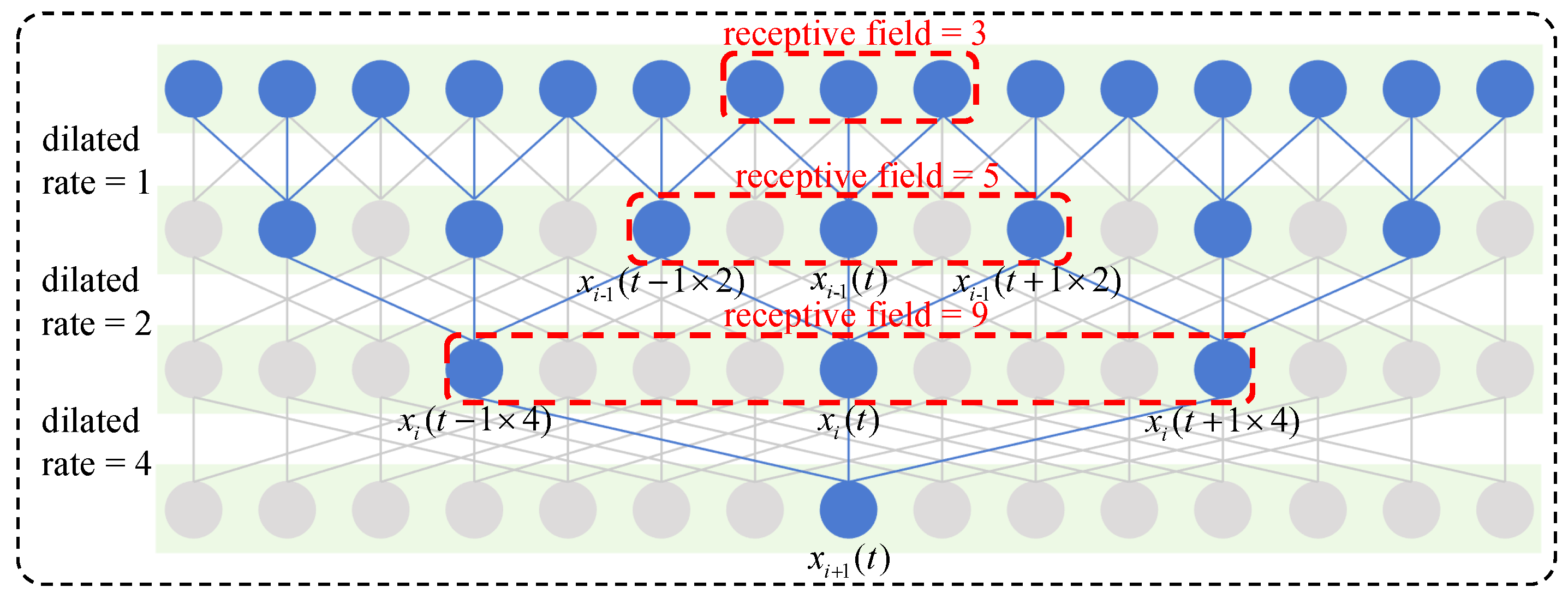
3.3. Temporal Convolutional Network (TCN)
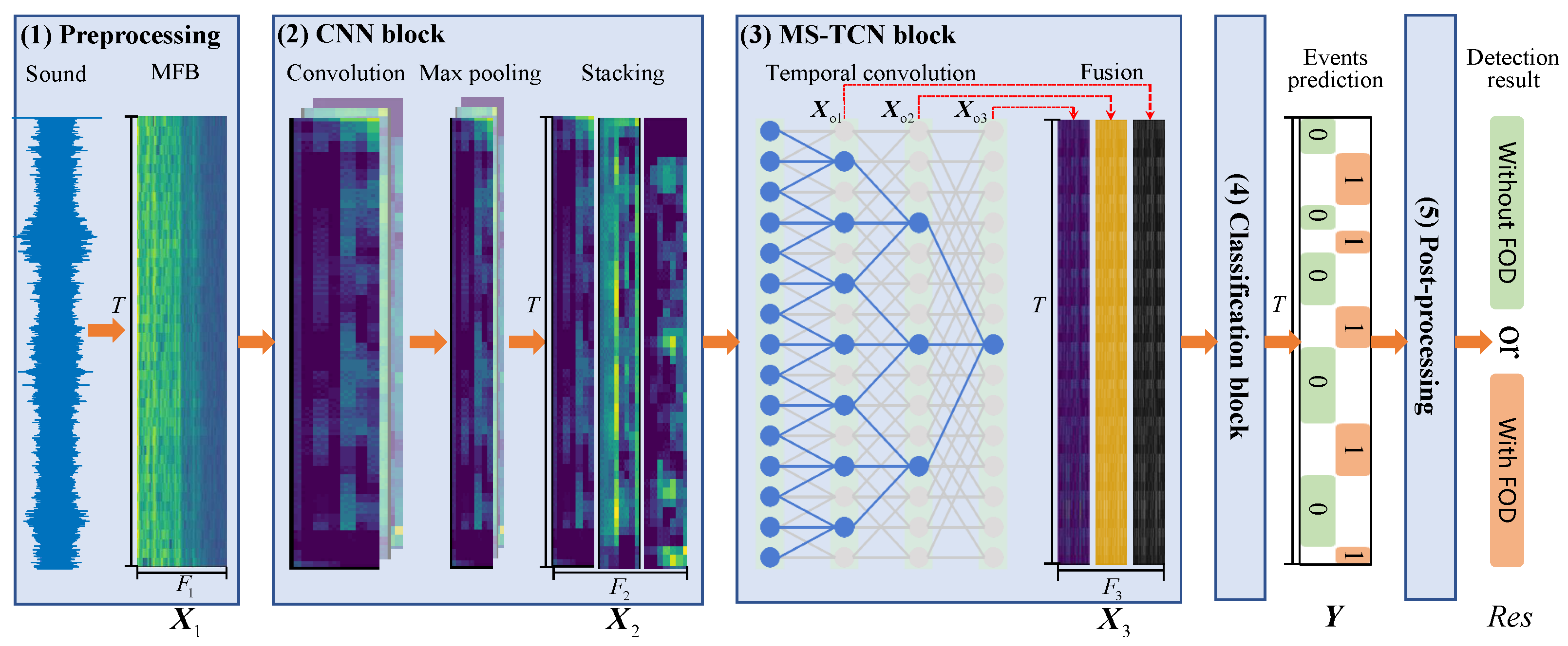
4. Proposed Method
4.1. Preprocessing
4.2. CNN Block
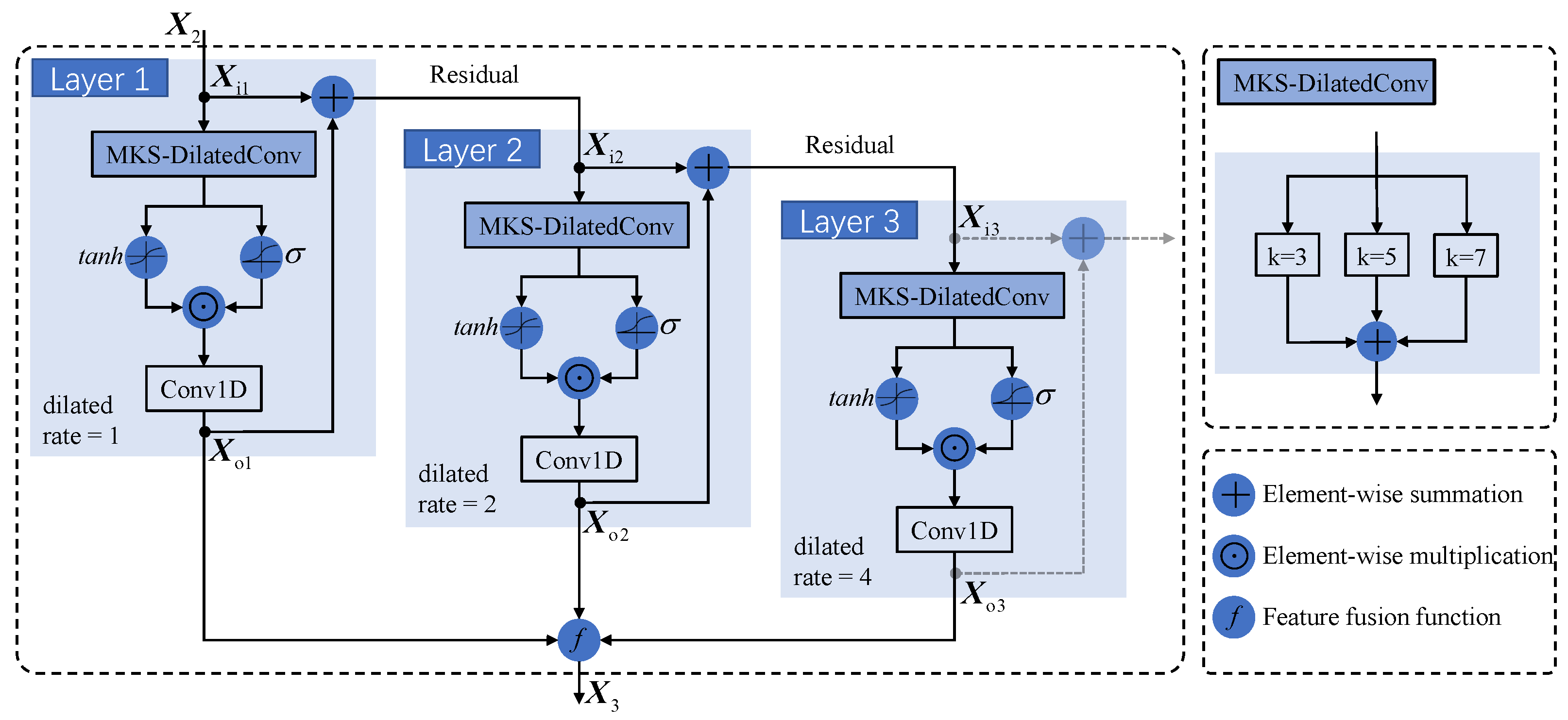
4.3. MS-TCN Block
4.4. Classification Block
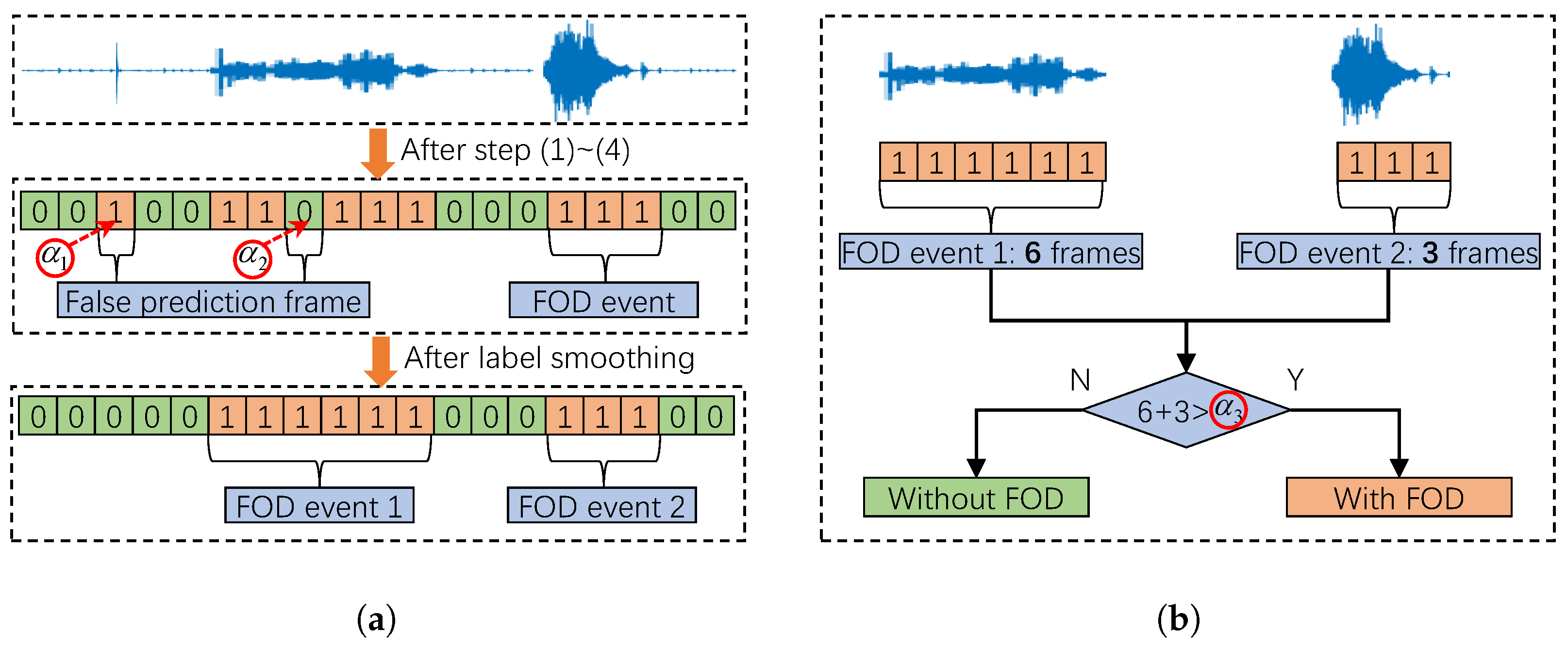
4.5. Post-Processing
| Algorithm 1: Post-processing |
| Input :prediction result , continuous threshold value , |
| interval threshold , allowable frame length threshold |
| Output: final detection result , where 0 and 1 denote normal and |
| abnormal respectively. |
 |
5. Experimental Setup
5.1. Signal and Data Description
5.2. Metrics
5.3. Comparison Methods and Parameter Setting
6. Results and Discussion
6.1. Overall Performance Analysis of MS-CTCN
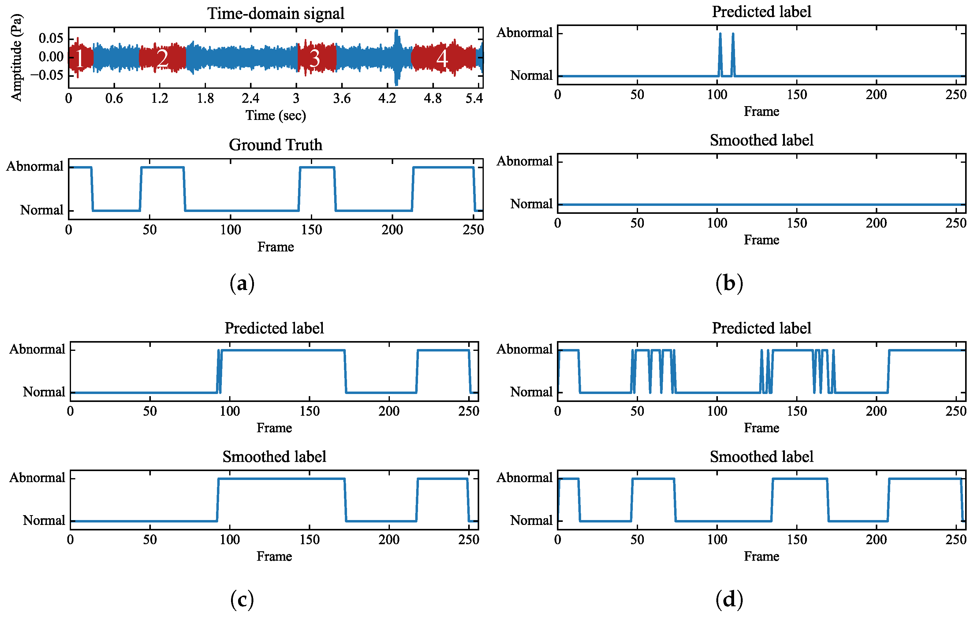
6.2. Frame-Wise Event Detection Performance Analysis
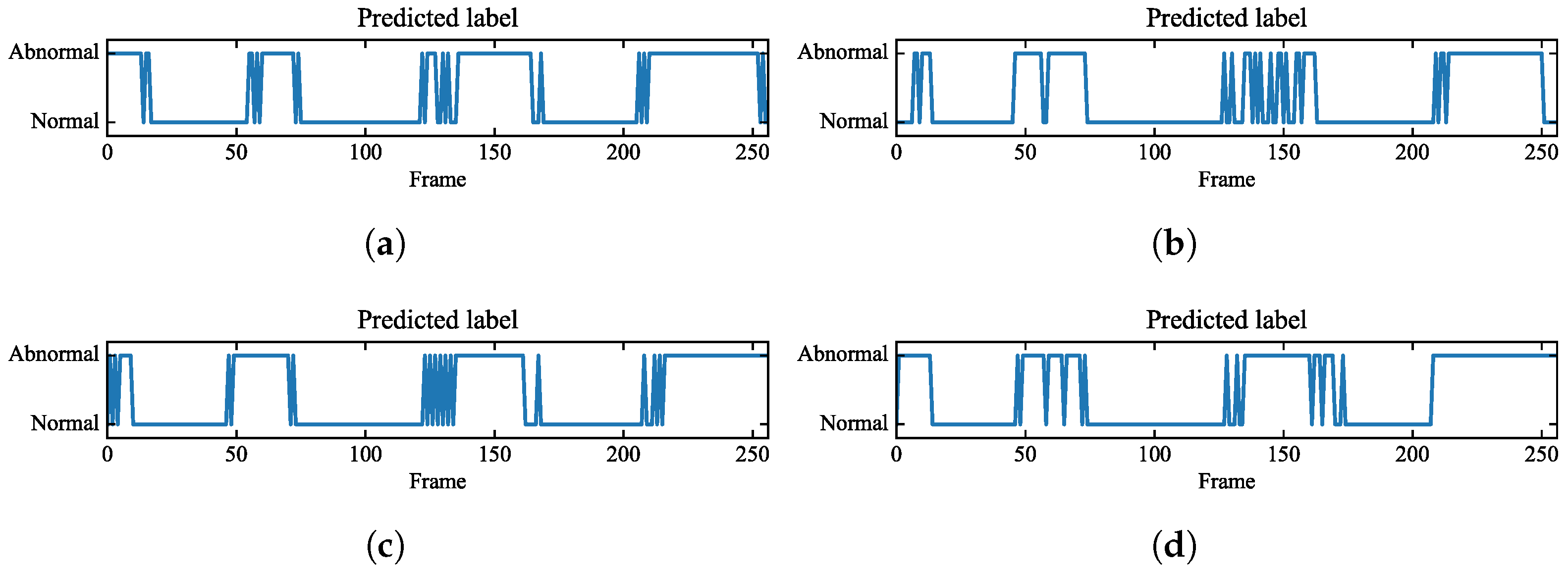
6.3. Performance of MS-TCN with Different Kernel Sizes
7. Conclusions
Author Contributions
Funding
Data Availability Statement
Conflicts of Interest
References
- Li, J.; Liang, G. Simulation of mass and heat transfer in liquid hydrogen tanks during pressurizing. Chin. J. Aeronaut. 2019, 32, 2068–2084. [Google Scholar] [CrossRef]
- Porto, J.F.D.; Loescher, D.H.; Olson, H.C.; Plunkett, P.V. SEM/EDAX Analysis of PIND Test Failures. In Proceedings of the 19th International Reliability Physics Symposium, Las Vegas, NV, USA, 7–9 April 1981; pp. 163–166. [Google Scholar] [CrossRef]
- Scaglione, L. Neural network application to particle impact noise detection. In Proceedings of the 1994 IEEE International Conference on Neural Networks (ICNN’94), Orlando, FL, USA, 28 June–2 July 1994; Volume 5, pp. 3415–3419. [Google Scholar] [CrossRef]
- Wang, S.; Chen, R.; Zhang, L.; Wang, S. Detection and material identification of loose particles inside the aerospace power supply via stochastic resonance and LVQ network. Trans. Inst. Meas. Control. 2012, 34, 947–955. [Google Scholar] [CrossRef]
- Zhai, G.; Chen, J.; Li, C.; Wang, G. Pattern recognition approach to identify loose particle material based on modified MFCC and HMMs. Neurocomputing 2015, 155, 135–145. [Google Scholar] [CrossRef]
- Wang, G.T.; Liang, X.W.; Xue, Y.Y.; Li, C.; Ding, Q. Algorithm Used to Detect Weak Signals Covered by Noise in PIND. Int. J. Aerosp. Eng. 2019, 2019, e1637953. [Google Scholar] [CrossRef] [Green Version]
- Gao, H.l.; Zhang, H.; Wang, S.j. Research on Auto-detection for Remainder Particles of Aerospace Relay Based on Wavelet Analysis. Chin. J. Aeronaut. 2007, 20, 75–80. [Google Scholar] [CrossRef] [Green Version]
- Wang, S.j.; Gao, H.l.; Zhai, G.f. Research on Feature Extraction of Remnant Particles of Aerospace Relays. Chin. J. Aeronaut. 2007, 20, 253–259. [Google Scholar] [CrossRef] [Green Version]
- Liu, Y.; Li, S.; Wang, J.; Zeng, H.; Lu, J. A computer vision-based assistant system for the assembly of narrow cabin products. Int. J. Adv. Manuf. Technol. 2015, 76, 281–293. [Google Scholar] [CrossRef]
- Xu, H.; Han, Z.; Feng, S.; Zhou, H.; Fang, Y. Foreign object debris material recognition based on convolutional neural networks. EURASIP J. Image Video Process. 2018, 2018, 21. [Google Scholar] [CrossRef]
- Wang, Y.S.; Liu, N.N.; Guo, H.; Wang, X.L. An engine-fault-diagnosis system based on sound intensity analysis and wavelet packet pre-processing neural network. Eng. Appl. Artif. Intell. 2020, 94, 103765. [Google Scholar] [CrossRef]
- Zhang, S.; He, Q.; Ouyang, K.; Xiong, W. Multi-bearing weak defect detection for wayside acoustic diagnosis based on a time-varying spatial filtering rearrangement. Mech. Syst. Signal Process. 2018, 100, 224–241. [Google Scholar] [CrossRef]
- Huang, Q.; Xie, L.; Yin, G.; Ran, M.; Liu, X.; Zheng, J. Acoustic signal analysis for detecting defects inside an arc magnet using a combination of variational mode decomposition and beetle antennae search. ISA Trans. 2020, 102, 347–364. [Google Scholar] [CrossRef] [PubMed]
- Tran, M.Q.; Liu, M.K.; Elsisi, M. Effective multi-sensor data fusion for chatter detection in milling process. ISA Trans. 2022, 125, 514–527. [Google Scholar] [CrossRef]
- Yao, Y.; Zhang, S.; Yang, S.; Gui, G. Learning Attention Representation with a Multi-Scale CNN for Gear Fault Diagnosis under Different Working Conditions. Sensors 2020, 20, 1233. [Google Scholar] [CrossRef] [Green Version]
- Parey, A.; Singh, A. Gearbox fault diagnosis using acoustic signals, continuous wavelet transform and adaptive neuro-fuzzy inference system. Appl. Acoust. 2019, 147, 133–140. [Google Scholar] [CrossRef]
- Zhang, G.; Wang, J.; Han, B.; Jia, S.; Wang, X.; He, J. A Novel Deep Sparse Filtering Method for Intelligent Fault Diagnosis by Acoustic Signal Processing. Shock Vib. 2020, 2020, e8837047. [Google Scholar] [CrossRef]
- Li, X.; Wan, S.; Liu, S.; Zhang, Y.; Hong, J.; Wang, D. Bearing fault diagnosis method based on attention mechanism and multilayer fusion network. ISA Trans. 2022, 128, 550–564. [Google Scholar] [CrossRef]
- Glowacz, A.; Glowacz, W.; Glowacz, Z.; Kozik, J. Early fault diagnosis of bearing and stator faults of the single-phase induction motor using acoustic signals. Measurement 2018, 113, 1–9. [Google Scholar] [CrossRef]
- Nakamura, H.; Asano, K.; Usuda, S.; Mizuno, Y. A Diagnosis Method of Bearing and Stator Fault in Motor Using Rotating Sound Based on Deep Learning. Energies 2021, 14, 1319. [Google Scholar] [CrossRef]
- Heittola, T.; Mesaros, A.; Eronen, A.; Virtanen, T. Context-dependent sound event detection. EURASIP J. Audio Speech Music. Process. 2013, 2013, 1. [Google Scholar] [CrossRef] [Green Version]
- Mesaros, A.; Heittola, T.; Dikmen, O.; Virtanen, T. Sound event detection in real life recordings using coupled matrix factorization of spectral representations and class activity annotations. In Proceedings of the 2015 IEEE International Conference on Acoustics, Speech and Signal Processing (ICASSP), South Brisbane, QLD, Australia, 19–24 April 2015; pp. 151–155. [Google Scholar] [CrossRef]
- Huang, G.; Heittola, T.; Virtanen, T. Using Sequential Information in Polyphonic Sound Event Detection. In Proceedings of the 2018 16th International Workshop on Acoustic Signal Enhancement (IWAENC), Tokyo, Japan, 17–20 September 2018; pp. 291–295. [Google Scholar] [CrossRef]
- Adavanne, S.; Politis, A.; Virtanen, T. Multichannel Sound Event Detection Using 3D Convolutional Neural Networks for Learning Inter-channel Features. In Proceedings of the 2018 International Joint Conference on Neural Networks (IJCNN), Rio de Janeiro, Brazil, 8–13 July 2018; pp. 1–7. [Google Scholar] [CrossRef] [Green Version]
- Li, Y.; Liu, M.; Drossos, K.; Virtanen, T. Sound Event Detection Via Dilated Convolutional Recurrent Neural Networks. In Proceedings of the ICASSP 2020—2020 IEEE International Conference on Acoustics, Speech and Signal Processing (ICASSP), Barcelona, Spain, 4–8 May 2020; pp. 286–290. [Google Scholar] [CrossRef] [Green Version]
- Yu, Y.; Si, X.; Hu, C.; Zhang, J. A Review of Recurrent Neural Networks: LSTM Cells and Network Architectures. Neural Comput. 2019, 31, 1235–1270. [Google Scholar] [CrossRef]
- Chung, J.; Gulcehre, C.; Cho, K.; Bengio, Y. Empirical Evaluation of Gated Recurrent Neural Networks on Sequence Modeling. arXiv 2014, arXiv:1412.3555. [Google Scholar] [CrossRef]
- Wang, Y.; Zhao, G.; Xiong, K.; Shi, G.; Zhang, Y. Multi-Scale and Single-Scale Fully Convolutional Networks for Sound Event Detection. Neurocomputing 2021, 421, 51–65. [Google Scholar] [CrossRef]
- Guirguis, K.; Schorn, C.; Guntoro, A.; Abdulatif, S.; Yang, B. SELD-TCN: Sound Event Localization & Detection via Temporal Convolutional Networks. In Proceedings of the 2020 28th European Signal Processing Conference (EUSIPCO), Amsterdam, The Netherlands, 18–21 January 2021; pp. 16–20. [Google Scholar] [CrossRef]
- Frigieri, E.P.; Brito, T.G.; Ynoguti, C.A.; Paiva, A.P.; Ferreira, J.R.; Balestrassi, P.P. Pattern recognition in audible sound energy emissions of AISI 52100 hardened steel turning: A MFCC-based approach. Int. J. Adv. Manuf. Technol. 2017, 88, 1383–1392. [Google Scholar] [CrossRef]
- Warren Liao, T. Feature extraction and selection from acoustic emission signals with an application in grinding wheel condition monitoring. Eng. Appl. Artif. Intell. 2010, 23, 74–84. [Google Scholar] [CrossRef]
- Brahim, J.; Loubna, R.; Noureddine, F. Rnn-And Cnn-Based Weed Detection For Crop Improvement: An Overview. Foods Raw Mater. 2021, 9, 387–396. [Google Scholar]
- Jabir, B.; Falih, N.; Rahmani, K. Accuracy and Efficiency Comparison of Object Detection Open-Source Models. Int. J. Online Biomed. Eng. (iJOE) 2021, 17, 165. [Google Scholar] [CrossRef]
- Zinemanas, P.; Cancela, P.; Rocamora, M. End-to-end Convolutional Neural Networks for Sound Event Detection in Urban Environments. In Proceedings of the 2019 24th Conference of Open Innovations Association (FRUCT), Moscow, Russia, 8–12 April 2019; pp. 533–539. [Google Scholar] [CrossRef]
- Wang, C.Y.; Tai, T.C.; Wang, J.C.; Santoso, A.; Mathulaprangsan, S.; Chiang, C.C.; Wu, C.H. Sound Events Recognition and Retrieval Using Multi-Convolutional-Channel Sparse Coding Convolutional Neural Networks. IEEE/ACM Trans. Audio Speech Lang. Process. 2020, 28, 1875–1887. [Google Scholar] [CrossRef]
- Khan, S.; Naseer, M.; Hayat, M.; Zamir, S.W.; Khan, F.S.; Shah, M. Transformers in Vision: A Survey. ACM Comput. Surv. 2022, 54, 200:1–200:41. [Google Scholar] [CrossRef]
- Imoto, K.; Kyochi, S. Sound Event Detection Utilizing Graph Laplacian Regularization with Event Co-Occurrence. Ieice Trans. Inf. Syst. 2020, E103.D, 1971–1977. [Google Scholar] [CrossRef]
- Kim, S.J.; Chung, Y.J. Multi-Scale Features for Transformer Model to Improve the Performance of Sound Event Detection. Appl. Sci. 2022, 12, 2626. [Google Scholar] [CrossRef]
- Kong, Q.; Xu, Y.; Wang, W.; Plumbley, M.D. Sound Event Detection of Weakly Labelled Data With CNN-Transformer and Automatic Threshold Optimization. IEEE/ACM Trans. Audio Speech Lang. Process. 2020, 28, 2450–2460. [Google Scholar] [CrossRef]
- D’Ascoli, S.; Touvron, H.; Leavitt, M.L.; Morcos, A.S.; Biroli, G.; Sagun, L. ConViT: Improving Vision Transformers with Soft Convolutional Inductive Biases. In Proceedings of the 38th International Conference on Machine Learning, PMLR, Virtual, 18–24 July 2021; pp. 2286–2296. [Google Scholar]
- Wang, J.J.; Wang, C.; Fan, J.S.; Mo, Y.L. A deep learning framework for constitutive modeling based on temporal convolutional network. J. Comput. Phys. 2022, 449, 110784. [Google Scholar] [CrossRef]
- Wang, Y.; Zhao, G.; Xiong, K.; Shi, G. MSFF-Net: Multi-scale feature fusing networks with dilated mixed convolution and cascaded parallel framework for sound event detection. Digit. Signal Process. 2022, 122, 103319. [Google Scholar] [CrossRef]
- Kopparapu, S.K.; Laxminarayana, M. Choice of Mel filter bank in computing MFCC of a resampled speech. In Proceedings of the 10th International Conference on Information Science, Signal Processing and their Applications (ISSPA 2010), Kuala Lumpur, Malaysia, 10–13 May 2010; pp. 121–124. [Google Scholar] [CrossRef] [Green Version]
- Allen, J.; Rabiner, L. A unified approach to short-time Fourier analysis and synthesis. Proc. IEEE 1977, 65, 1558–1564. [Google Scholar] [CrossRef]
- Tak, R.N.; Agrawal, D.M.; Patil, H.A. Novel Phase Encoded Mel Filterbank Energies for Environmental Sound Classification. In Proceedings of the Pattern Recognition and Machine Intelligence; Shankar, B.U., Ghosh, K., Mandal, D.P., Ray, S.S., Zhang, D., Pal, S.K., Eds.; Lecture Notes in Computer Science; Springer International Publishing: Cham, Switzerland, 2017; pp. 317–325. [Google Scholar] [CrossRef]
- Li, Y.; Du, X.; Wan, F.; Wang, X.; Yu, H. Rotating machinery fault diagnosis based on convolutional neural network and infrared thermal imaging. Chin. J. Aeronaut. 2020, 33, 427–438. [Google Scholar] [CrossRef]
- Vafeiadis, A.; Votis, K.; Giakoumis, D.; Tzovaras, D.; Chen, L.; Hamzaoui, R. Audio content analysis for unobtrusive event detection in smart homes. Eng. Appl. Artif. Intell. 2020, 89, 103226. [Google Scholar] [CrossRef] [Green Version]
- Hasan, M.J.; Islam, M.M.M.; Kim, J.M. Acoustic spectral imaging and transfer learning for reliable bearing fault diagnosis under variable speed conditions. Measurement 2019, 138, 620–631. [Google Scholar] [CrossRef]
- Hasan, M.J.; Islam, M.M.M.; Kim, J.M. Multi-sensor fusion-based time-frequency imaging and transfer learning for spherical tank crack diagnosis under variable pressure conditions. Measurement 2021, 168, 108478. [Google Scholar] [CrossRef]
- Ioffe, S.; Szegedy, C. Batch Normalization: Accelerating Deep Network Training by Reducing Internal Covariate Shift. arXiv 2015. [Google Scholar] [CrossRef]
- Jiao, J.; Zhao, M.; Lin, J.; Liang, K. A comprehensive review on convolutional neural network in machine fault diagnosis. Neurocomputing 2020, 417, 36–63. [Google Scholar] [CrossRef]
- Biscione, V.; Bowers, J. Learning Translation Invariance in CNNs. arXiv 2020. [Google Scholar] [CrossRef]
- Sainath, T.N.; Vinyals, O.; Senior, A.; Sak, H. Convolutional, Long Short-Term Memory, fully connected Deep Neural Networks. In Proceedings of the 2015 IEEE International Conference on Acoustics, Speech and Signal Processing (ICASSP), South Brisbane, QLD, Australia, 19–24 April 2015; pp. 4580–4584. [Google Scholar] [CrossRef]
- Oord, A.v.d.; Dieleman, S.; Zen, H.; Simonyan, K.; Vinyals, O.; Graves, A.; Kalchbrenner, N.; Senior, A.; Kavukcuoglu, K. WaveNet: A Generative Model for Raw Audio. arXiv 2016. [Google Scholar] [CrossRef]
- He, K.; Zhang, X.; Ren, S.; Sun, J. Deep Residual Learning for Image Recognition. In Proceedings of the 2016 IEEE Conference on Computer Vision and Pattern Recognition (CVPR), Las Vegas, NV, USA, 27–30 June 2016; pp. 770–778. [Google Scholar] [CrossRef] [Green Version]
- Mesaros, A.; Heittola, T.; Virtanen, T. Metrics for Polyphonic Sound Event Detection. Appl. Sci. 2016, 6, 162. [Google Scholar] [CrossRef] [Green Version]
- Gao, D.W.; Zhu, Y.S.; Yan, K.; Fu, H.; Ren, Z.J.; Kang, W.; Guedes Soares, C. Joint learning system based on semi–pseudo–label reliability assessment for weak–fault diagnosis with few labels. Mech. Syst. Signal Process. 2023, 189, 110089. [Google Scholar] [CrossRef]
- Shaw, A.; Smith, J.; Hassanien, A. MVDR Beamformer Design by Imposing Unit Circle Roots Constraints for Uniform Linear Arrays. IEEE Trans. Signal Process. 2021, 69, 6116–6130. [Google Scholar] [CrossRef]


| Acoustic Condition of the Tank | Number of the Training Samples | Number of the Testing Samples | |
|---|---|---|---|
| With FOD (abnormal) | Nut | 960 | 240 |
| Ti-wire (3.39 g) | 960 | 240 | |
| Ti-wire (0.33 g) | 960 | 240 | |
| Rivet | 960 | 240 | |
| Bolt | 960 | 240 | |
| Without FOD (normal) | - | - | 1200 |
| Total | - | 4800 | 2400 |
| Operation | Output Size | Configuration |
|---|---|---|
| Preprocessing | 256 × 128 | - |
| Network input | 1 × 256 × 128 | - |
| CNN1(32, 5, 5) | 32 × 256 × 128 | Max-pooling (1, 4) |
| CNN2(32, 5, 5) | 32 × 256 × 32 | Max-pooling (1, 4) |
| CNN3(32, 3, 3) | 32 × 256 × 4 | Max-pooling (1, 2) |
| Reshape | 256 × 128 | - |
| TCN1 | 256 × 128 | Dilation rate = 1 |
| TCN2 | 256 × 128 | Dilation rate = 2 |
| TCN3 | 256 × 128 | Dilation rate = 4 |
| Connection | 256 × 384 | - |
| FC1 | 256 × 128 | - |
| FC2 | 256 × 2 | - |
| Sigmoid | 256 × 2 | - |
| Post-processing | 1 | , , |
| Model | P(%) | R(%) | F(%) | Ptotal(%) |
|---|---|---|---|---|
| CNN | 100 | 0.08 | 0.17 | 50.04 |
| CRNN | 99.12 | 93.75 | 96.36 | 96.46 |
| MS-CTCN | 99.41 | 98.82 | 99.17 | 99.16 |
| Type of FOD | CRNN(%) | MS-CTCN(%) |
|---|---|---|
| Nut | 100 | 100 |
| Ti-wire (3.93) | 100 | 100 |
| Ti-wire (0.33) | 77.50 | 97.92 |
| Rivet | 93.75 | 97.50 |
| Bolt | 100 | 100 |
| Model | P(%) | R(%) | F(%) |
|---|---|---|---|
| KS-3 | 99.82 | 99.67 | 98.22 |
| KS-5 | 99.74 | 96.00 | 97.83 |
| KS-7 | 99.82 | 96.08 | 97.91 |
| MKS | 99.40 | 98.92 | 99.16 |
Disclaimer/Publisher’s Note: The statements, opinions and data contained in all publications are solely those of the individual author(s) and contributor(s) and not of MDPI and/or the editor(s). MDPI and/or the editor(s) disclaim responsibility for any injury to people or property resulting from any ideas, methods, instructions or products referred to in the content. |
© 2023 by the authors. Licensee MDPI, Basel, Switzerland. This article is an open access article distributed under the terms and conditions of the Creative Commons Attribution (CC BY) license (https://creativecommons.org/licenses/by/4.0/).
Share and Cite
Lin, T.; Zhu, Y.; Ren, Z.; Huang, K.; Zhang, X.; Yan, K.; Huang, S. Sound-Based Intelligent Detection of FOD in the Final Assembly of Rocket Tanks. Machines 2023, 11, 187. https://doi.org/10.3390/machines11020187
Lin T, Zhu Y, Ren Z, Huang K, Zhang X, Yan K, Huang S. Sound-Based Intelligent Detection of FOD in the Final Assembly of Rocket Tanks. Machines. 2023; 11(2):187. https://doi.org/10.3390/machines11020187
Chicago/Turabian StyleLin, Tantao, Yongsheng Zhu, Zhijun Ren, Kai Huang, Xinzhuo Zhang, Ke Yan, and Shunzhou Huang. 2023. "Sound-Based Intelligent Detection of FOD in the Final Assembly of Rocket Tanks" Machines 11, no. 2: 187. https://doi.org/10.3390/machines11020187