Explainable Data-Driven Method Combined with Bayesian Filtering for Remaining Useful Lifetime Prediction of Aircraft Engines Using NASA CMAPSS Datasets

Abstract

An aircraft engine is expected to have a high-reliability system as a safety-critical asset. A scheduled maintenance strategy based on statistical calculation has been employed as the current practice to achieve the reliability requirement. Any improvement to this maintenance interval is made after significant reliability issues arise (such as flight delays and high component removals). Several publications and research studies have been conducted related to this issue, one of them involves performing simulations and providing aircraft operation datasets. The recently published NASA CMAPPS datasets have been utilised in this paper since they simulate flight data recording from various measurements. A prognostics model can be developed by analysing these datasets and predicting the engine’s reliability before failure. However, the state-of-the-art prognostics techniques published in the literature using these NASA CMAPPS datasets are mainly purely data-driven. These techniques mainly deal with a “black box” process which does not include uncertainty quantification (UQ). These two factors are barriers to prognostics applications, particularly in the aviation industry. To tackle these issues, this paper aims at developing explainable and transparent algorithms and a software tool to compute the engine health, estimate engine end of life (EoL), and eventually predict its remaining useful life (RUL). The proposed algorithms use hybrid metrics for feature selection, employ logistic regression for health index estimation, and unscented Kalman filter (UKF) to update the prognostics model for predicting the RUL in a recursive fashion. Among the available datasets, dataset 02 is chosen because it has been widely used and is an ideal candidate for result comparison and dataset 03 is employed as a new state-of-the-art. As a result, the proposed algorithms yield 34.5–55.6% better performance in terms of the root mean squared error (RMSE) compared with the previous work. More importantly, the proposed method is transparent and it quantifies the uncertainty during the prediction process.

1. Introduction

1.1. Background

As a safety-critical asset, aircraft are expected to have high reliability and airworthy conditions. Due to this requirement, it is a big challenge to keep a high availability in the aircraft fleet. Any unforeseen technical problems may lead to operational interruptions (e.g., flight delays, air-turn-back), leading to costly downtime (e.g., aircraft on the ground), or even fatal accidents. Thus, airlines devise various maintenance strategies to avoid these events and to optimised the aircraft fleet up-time.

Most airlines use maintenance planning documents (MPDs) as their base. MPDs are set by aircraft manufacturers which mostly refer to Maintenance Steering Group 3 (MSG-3) [1]. It is a combination of reactive maintenance (for expendable parts), preventive maintenance (for critical components), and condition-based maintenance (for repairable components), and these tasks are included in the aircraft maintenance program (MP).

During the aircraft’s lifetime, the MP is evolving to keep the aircraft serviceable and airworthy [2]. Airlines can add other maintenance tasks that are not covered by MP. In this case, they have to determine the maintenance interval for these additional tasks. Several methods are employed to find the optimum interval but mostly based on the pre-defined interval (such as A-check, C-check) [1]. The quantitative approach, such as statistical by using Weibull analysis, is also commonly used to determine the optimum interval for time-based preventive maintenance.

However, the statistical calculation mostly takes into account the population or fleet data. The drawback of this approach is the uncertainty which means some components may fail before the calculated time, thus the unplanned breakdown still occurs, as seen in Figure 1 (left side). On the other hand, there is a high possibility of unnecessary replacement where a usable component is removed before it breaks down. This early intervention can cause an opportunity loss because it does not fully utilise the component’s useful life (Figure 1, right side).

Prognostics and Health Management (PHM) is introduced to alleviate this issue. PHM is a holistic approach utilising sensor data for the maintenance decision to optimise asset value. In [3], the PHM functional architecture involves three major phases: data acquisition, interpretation, and maintenance management. The data acquisition phase involves collecting data from multiple sensors and pre-processing the relevant parameters or features from the raw data. The interpretation phase analyses the pre-processed data to detect operation anomaly (first level), assess system health and diagnose the failure mode (second level), and predict the asset remaining useful life (third level). All these interpretations provide valuable information for the maintenance management phase, where informed maintenance decisions (tactical control or strategic planning) are taken.

In the aviation industry, the maintenance approach is rapidly evolving from preventive to condition-based maintenance (CBM) and/or predictive maintenance (PdM) [4]. In the preventive maintenance approaches, maintenance action (replacement, inspection, data collection) is often taken within a specific interval (time-based). However, it lacks the capability of individual asset assessment since each asset may behave differently under different loads or operating conditions. Prognostics aims to solve this problem by predicting the system state and reliability of each asset and its estimated failure time, and providing confidence and valuable information to the operators [5]. This information proves beneficial to the operator because maintenance intervention is only performed when needed [6].

However, the prognostics model requires sufficient degradation data to make a good prediction. Nevertheless, this is not always the case with aircraft systems. Due to its criticality, aircraft manufacturers intentionally produce highly reliable components which leads to scarce “run-to-fail” data. Hence, a fully implemented prognostics model is still rare in the aviation industry. On the other hand, the RUL prediction in prognostics is not certain and not always 100% accurate. This uncertainty becomes more crucial for safety-critical assets, especially for aircraft. Thus, the RUL prediction implementation complemented by uncertainty quantification is desirable.

1.2. Related Works

The CBM approach increases system reliability by calling maintenance actions based on the state of the asset. Within the CBM context, diagnostics are involved in diagnosing asset faults [7]. While CBM deals with the sensor data, detecting, isolating, and identifying the faults (severity and degradation detection) [8], PdM is the next process, where prognostics is involved, which estimates the time-to-failure (degradation prediction and condition indicator trend) or remaining useful life (RUL) before the asset fails [9]. It indicates that both processes are overlapped, where prognostics also requires diagnostics in the early phase [10].

There are two main categories in developing prognostics models: The physics-based model (PbM) and data-driven model (DdM). The summaries of the PbM and DdM are provided in

Table 1. Physics-based Model (PbM) vs. Data-driven Model (DdM).

Prognostics Model	Advantages	Disadvantages
Physics-based	Higher accuracy	Require expertise in failure mechanism
	Require less data	Applies only for specific systems (not scalable)
	Able to represent a different operational	Higher cost
Data-driven	Flexible and adaptable to complex dataset	Require sufficient run-to-fail data
	Relatively easier to develop	A more complex computational process
	Can be applied to the next-higher level (scalable)	Determine the failure threshold can be challenging
	Lower cost

. The PbM requires a mathematical equation derived from the first principle of asset degradation, such as crack growth modeling [10], and it requires expertise and knowledge about the system [11]. The PbM can provide an excellent prediction if the mathematical model accurately represents the degradation process. It can be a robust solution with less training data and describe various operational conditions [12]. However, the PbM can only apply to a specific component or system [10], and it requires more cost compared to other methods [13].

The data-driven model (DdM) gives an alternative approach to detecting system degradation provided sufficient run-to-failure data or samples. Generally, the statistical approach and artificial intelligence (AI) are the standard methods for DdM [10]. In the statistical approach, a prediction model can be constructed by fitting a probabilistic model to the observed data, such as the Markovian process-based model, regression model, or independent increment process-based Model [14]. Machine learning (ML) is an example of an AI approach to building prognostics models. ML can recognise a complex pattern and make a decision based on the available data from sensors [10]. Artificial neural networks (ANN) [6], convolutional neural networks (CNN) [15], tree-based such as random forests [16], support vector machines (SVM) [17], and self-organising maps [10] are typical ML approaches in prognostics.

Tsui et al., 2015 [14] categorised the major data-driven prognostics, such as independent increment process-based models, Markovian process-based models, filtering-based models, regression-based models, proportional hazard models, and threshold regression models. One of the model-based prognosis problems is how to estimate a joint state parameter of the asset. This problem is typically solved by using filtering-based models [18]. The state-parameter distribution is simulated to predict the machine’s end-of-life and RUL.

Most prognostics research in aviation acquired and utilised data from the NASA repository. The latest development of aircraft engine commercial modular aero-propulsion system simulation (CMAPSS) datasets was publicly released in 2021 [19]. These novel datasets are the upgrade of the previous similar datasets that were published in 2008 [20]. While data from laboratory experiments and simulations may not describe real flight conditions [21], the new CMAPSS data incorporate two levels of fidelity by considering the real flight condition and extending the degradation model based on operation history [19].

To the best of the author’s knowledge, there are five previous publications on the new dataset since 2021. Two of them discuss dataset documentation [19] and exploratory data analysis [22] of the dataset. The other publications attempt to develop a prognostics model by using an ML model, namely spiking neural P [23] and anticausal learning [24], and the deep Gaussian process [25].

1.3. Aim, Objectives and Main Contributions

This paper aims to provide a methodology and algorithm for an aircraft engine’s condition monitoring and prognostics system. The latest NASA CMAPSS datasets are used as training and test datasets to validate the estimated RULs. The RUL estimates can then be used for maintenance decisions, such as maintenance intervention, planning and scheduling, and parts preparation. To achieve this aim, the objectives of this paper are divided as follows:

• To investigate the current state-of-the-art of prognostics technology.
• To develop condition monitoring and prognostics algorithms and software tools for improved aircraft engine maintenance.

A limited number of researchers employed the latest CMAPSS dataset for prognostic purposes. While ML is the main proposed approach in these publications, a few discussed other data-driven techniques in prognostics. Most of these AI approaches deal with a “black box” nature, which does not provide any clue about the internal processes and the output confidence level, which is especially an issue for high-risk assets, such as aircraft engines. On the other hand, the challenge of quantifying the level of uncertainty is still one of the biggest barriers for prognostics applications in the industry. Hence, this paper intends to tackle the aforementioned issue by providing alternative techniques, and fill the research and industrial gap while maintaining good RUL prediction performance.

The main contributions of this paper are:

• Offers an alternative prognostics technique to the published data-driven approaches of the latest CMAPSS dataset with a high level of transparency and uncertainty quantification.
• Attempts to proximate the prognostics application in the industry considering limited data availability, transparency, and safety-critical nature (e.g., aircraft engines).
• CMAPSS dataset 02 is analysed and the prediction performance is compared to the published research results.
• Analysis of dataset 03 is employed as a new state-of-the-art.

1.4. Paper Organisation

This paper consists of four sections, namely Introduction, Methodology, Results and Discussion, and Conclusions and Future Work. Section 1 provides the background that motivates the research and previous research, and is followed by the aims and objectives, and how this paper contributes to prognostics technology development endeavour. The methodical steps taken for this paper are discussed in Section 2, including the tools and techniques used. The outcomes and findings are presented and the detailed investigation and evaluation of the results are the primary content of Section 3. The final part of this paper brings the key research points in Section 4; the summary and possible improvements are added for future research reference.

2. Methodology

2.1. Overview

The method followed in this paper is divided into six phases with different key tasks and outputs. Figure 2 shows the overall research methodology and each process is explained in the following sections. Notably, the algorithms are developed using Python version 3.9.7 with its latest packages for Data Acquisition, Feature Selection, Engine Prognostics, Parameter Tuning, and Performance Tests. Matlab R2021 version is used to build the engine condition monitoring algorithm.

2.2. Dataset

The relevant dataset acquisition phase is performed by accessing the latest aircraft engine data from the NASA repository. The latest CMAPSS data consider the real flight conditions and extend the degradation modelling [19]. Hence, these data are a favourable option for this paper. Among the available datasets in CMAPSS 2021, datasets 02 (DS02) and 03 (DS03) are chosen due to several factors. DS02 is the latest dataset in the current PHM challenge, which means it has been widely used and is an ideal candidate for result comparison. DS03 provides higher complexity since it covers more engine data, and it is perfect for training and testing during algorithms development. While the rest of the engines are used for algorithm training, three engines become the test units (11,14,15 for DS02, and 13,14,15 for DS03) for the performance test.

2.3. Feature Selection

In the Feature Selection phase, data dimensionality is reduced to decrease the computational power needed and to identify the critical features (parameters) contributing to the engine’s performance. This is because the chosen datasets (DS02 and DS03) are in h5 format and considered big data, with approximately 6 to 9 million data points for each engine. Such big data require high computational power, which is not ideal for simultaneous and continuous analysis. This paper employs several metrics acting as filters to select particular feature(s) that comply with the threshold requirement. Determining these metrics is crucial since it affects the complexity of prognostics modelling and prediction accuracy [26]. Several metrics are used in this paper due to their suitability for a single HI requirement and time-based dataset, namely Robustness, Monotonicity, and Prognosability.

When an engineering asset exhibits a stochastic process, a good feature should be robust to outliers and noise [27]. Hence, the Robustness metric has been introduced to check how robust the feature of interest is. Let $T=[t_1,t_2,\dots ,t_n,\dots t_N]$ and $X=[x_1,x_2,\dots ,x_n,\dots ,x_N]$ be the time and feature vectors, respectively, and N is the number of measurement. In [28], the robustness of a feature X is defined as:

$$Rob\left(X\right)=\frac{1}{N}\sum _{n=1}^{N}exp\left(-\left|\frac{x_n-\overline{x_n}}{x_n}\right|\right)$$

(1)

where $x_n$ is the feature value at the time index $t_n$ and $\overline{x_n}$ is the mean trend value of the feature which is acquired through smoothing process.

While the stochastic process may create arbitrary measurement values for each cycle, it has to show a degradation by showing an increasing and decreasing trend over time. The Monotonicity metric evaluates this trend information and shows which feature has degradation information of the asset [29]. There must be a correlation between the HI and time, and the selected features must show this correlation. Since most machinery presents non-linear degradation, the absolute value of the Spearman correlation is chosen because it can transform the non-linear into a linear relationship between HI and time [26]. Hence, the Monotonicity metric is mathematically expressed [30] as:

$$Mon(X,T)=\rho =\left|1-\frac{6{\sum }_{n=1}^N(\widetilde{X_n}-\widetilde{T_n})}{N(N^2-1)}\right|$$

(2)

where $\widetilde{X_n}$ and $\widetilde{T_n}$ are the rank sequence of X and T.

Prognosability is a desirable metric since it shows the different EoL is consistent across the fleet. This variance is measured by calculating the selected feature’s performance in predicting EoL at the same measurement level [31]. Formally, Prognosability is formulated as:

$$Prog\left(X\right)=exp\left(-\frac{std\left(X_j\left(N_j\right)\right)}{mean\left|X_j\left(1\right)-X_j\left(N_j\right)\right|}\right)$$

(3)

where j is the engine number, $X_j$ is measurement values of the features and $N_j$ is the number of measurement of engine j.

However, a single metric is insufficient to select suitable features sometimes. Thus, the Hybrid Metric ($HM$) is proposed to combine previous metrics (Robustness, Monotonicity, and Prognosability). The hybrid techniques can handle various properties of each singular metric and make a trade-off among different properties [26]. The formulation of the hybrid metric is a linear equation, and an equal weight is assigned for the three metrics, as shown in Equation (4) below. Since T is deterministic and irreversible, then X is the only variable in Monotonicity ($Mon$) in Equation (4). Nevertheless, T is still calculated in this equation since it deals with time-series data.

$$HM\left(X\right)=\frac{1}{3}Rob\left(X\right)+\frac{1}{3}Mon\left(X\right)+\frac{1}{3}Prog\left(X\right)$$

(4)

2.4. Features Fusion and Health Index Estimation

The Health Index Estimation phase focuses on fusing and translating information from the selected features into a dichotomy between healthy and failed. This method can estimate the engine health index as an indicator for condition monitoring. It is necessary to extract information from the selected features (F) and correlate this information to engine degradation to obtain the engine health state. In order to achieve this goal, this paper follows these steps: data sampling, performing regression on the sample data, and transforming all measurement data into a uniform scale (from 0 to 1), as shown in Figure 3.

In [32], logistic regression is chosen for features fusion, and it is also a suitable technique for dichotomous problems, where the predicted value is between 0 and 1. This approach is relevant and applied to this paper since the binary value (0 or 1) gives intuitive nature to the engine’s healthiness. A simple logistic function is defined as:

$$P\left(F\right)=h=\frac{1}{1+e^{-g\left(F\right)}}=\frac{e^{g\left(F\right)}}{1+e^{g\left(F\right)}}$$

(5)

where F is a set of selected features, h represents the engine HI, and g(F) is the logit function which is denoted as:

$$g\left(F\right)=g=log\left(\frac{P\left(F\right)}{1-P\left(F\right)}\right)=\sum _{i=0}^L{\beta }_i{F}_i$$

(6)

where L is the number of features.

The logit function expresses the “odds-off-success” from the probability function (logistic function). In the logit function, the log odds of the outcome are modelled as a linear combination of the selected features (F), and this function preserves the nature of these features (measurement signals) [32]. The logistic regression is employed to identify the logit function parameters $\left({\beta }_i\right)$, so the logistic model can be implemented to estimate the health assessment. This health assessment, shown by engine health index (HI) values from 1 (healthy) and 0 (failure), becomes the base for engine condition monitoring.

The engine end-of-life (EoL) prediction and remaining useful life (RUL) is the main objective in the RUL Prediction phase. As discussed in the previous Section 1.2, CBM and prognostics are strongly correlated. CBM is a necessary process to detect degradation and assess engine health state. Thus, the logistic regression from the previous section becomes the base for the prediction model.

The selected features (F) are the predictor variable, and the engine HI is the response variable. There are several possible distributions of the response variable: Normal, Binomial, Poisson, Gamma, and Inverse Gaussian. This paper explores each distribution by calculating the fitting’s root-mean-square error (RMSE). RMSE is a standard statistical metric for evaluating models [33], as shown in the Equation (7). The distribution that yields the lowest RMSE is the candidate for the following process.

$$RMSE=\sqrt{\frac{1}{N}\sum _{n=1}^N{(y_n-{\overline{y}}_n)}^2}$$

(7)

where N is number of observations (y) and the corresponding mean value ($\overline{y}$).

The Generalised Linear Model (GLM) is a flexible generalisation of linear regression that provides a linear relationship between more than one independent predictor variables ($x_j$) and one response variable (y) [34]. The GLM model is expressed as:

$$f\left(y\right)={\beta }_0+{\beta }_1{x}_1+{\beta }_2{x}_2+...+{\beta }_j{x}_j$$

(8)

$$\alpha ={\beta }_0$$

(9)

where ${\beta }_j$ is the regression coefficient of the independent variable, and f(y) uses a logistic function as the fitting model, instead of using a link function. As the result of GLM fitting, logistic regression coefficients ($\alpha$ and $\beta$) for each engine are determined. Each coefficient’s average ($\overline{\alpha }$ and $\overline{\beta }$) values are computed as a representation of the fleet for the next process.

2.5. Prognostics Algorithm

The condition monitoring and the mathematical model from GLM fitting can identify the engine’s current state. However, both have their own noise that affects the prediction performance. Thus, it is challenging to find the optimised value from this joint state. This problem is typically solved by using filtering-based models [18]. The state-parameter distribution is simulated to predict the machine’s EoL and RUL. Assuming the noise is both normally distributed, the Kalman filter (KF) is an efficient method to estimate the state of a system given a sequence measurement and times, a mathematical model describing system dynamic, and a model that corresponds to measurement value [35,36]. The KF is optimal for handling the linear transformation of both systems dynamic and measurement models. The unscented Kalman filter (UKF) is a derivation of the KF to handle nonlinear transformation by performing unscented transform (UT) and calculating the Kalman Gain for the predicted state in the next cycle [37].

The UKF is applied for the prognostics model since both engine system dynamic (from GLM fitting) and condition monitoring (logistic regression) are not linear. The mathematical model of UKF implementation is described in the following equations.

$$X_0^{+}=\left\{\begin{array}{c}\overline{\alpha }\\ \overline{\beta }\end{array}\right\}$$

(10)

$$P_0^{+}=\lambda .Cov(\alpha ,\beta )$$

(11)

$X_0^{+}$ is the initial state matrix, and $P_0^{+}$ is the initial covariance matrix for UKF. $X_0^{+}$ is the mean of each coefficient from GLM fitting, and $P_0^{+}$ is the covariance of coefficients of all training engines. Lambda ($\lambda$) is the scaling parameter for the UT process. The prediction and update phase of UKF is computed as follows:

$$\left\{\begin{array}{c}{\alpha }_k\\ {\beta }_k\end{array}\right\}=\left\{\begin{array}{cc}1& 0\\ 0& 1\end{array}\right\}\left\{\begin{array}{c}{\alpha }_{k-1}\\ {\beta }_{k-1}\end{array}\right\}+\left\{\begin{array}{c}{q}_{k-1}\\ q_{k-1}\end{array}\right\}$$

(12)

$$H{I}_k=\frac{1}{1+e^{{\alpha }_{k}N+{\beta }_k}}+v_k$$

(13)

where ${\alpha }_k$ and ${\beta }_k$ are the system coefficient for the prognostics model, both are recursively updated at step k whenever new measurement and system updates are available during cycle N. Measurement noise (v) and process noise (q) are considered to estimate the best approximation of the actual state value.

The updated coefficients (${\alpha }_k$ and ${\beta }_k$) are then used to extrapolate the prognostics models and predict the possible EoL. Uncertainty is computed by generating 1000 random trajectory samples and calculating the predicted RUL. Then, the distribution of predicted RUL is presented with a 90% confidence interval. This transparent process allows for adjusting the algorithms to optimise the results.

The transparent nature of the algorithm is exploited in the Parameter Tuning phase by adjusting the scaling parameter ($\lambda$) and EoL threshold to obtain the optimum prediction result. The explicit process in the UKF involves unscented transform (UT), where it is influenced by the $\lambda$ (see Equation (11)). Adjusting the $\lambda$ will alter the spread of the sigma points around the mean ($\overline{x}$[38] and affect the prediction-update process in UKF. One can optimise the prediction and minimise the resulting error by plotting the range $\lambda$ and comparing it to p score, as shown in Figure 4.

The threshold also needs to be adjusted to accommodate the expected EoL of the fleet. All EoL of each engine will be plotted to see the distribution. The distribution plot is necessary prior to the adjustment to see how EoL varies across the fleet.

In this paper, the comparison between EoL mean, max, and statistical process control (SPC), with 3$\sigma$, 2$\sigma$, and 1$\sigma$, are presented. SPC is a great tool to monitor the performance of a process over time to remain close to the desired values [39]. The EoL threshold adjustment depends on how critical the asset is and how conservative the maintenance strategy is. Given the high criticality of aircraft engines, it is best to be conservative in determining the EoL threshold. Hence, the chosen method is the one that gives the optimum prediction result even though it shows a higher threshold value.

2.6. Performance Test and Benchmark

Lastly, the Performance Test phase evaluates the algorithm by performing prediction on the test dataset. NASA scoring (s)and RMSE (e) are used as the metrics to check RUL prediction accuracy [19]. The s and e are defined as

$$s=\sum _{n=1}^{N}exp\left(\gamma \left|{\Delta }^{\left(n\right)}\right|\right)$$

(14)

$$e=\sqrt{\frac{1}{N}\sum _{n=1}^N{\left({\Delta }^{\left(n\right)}\right)}^2}$$

(15)

where N is the total number of the data sample, $\Delta$ is the difference between the predicted and the actual RUL of the n sample, and $\gamma$ is $\frac{1}{10}$ if RUL is over-estimated and $\frac{1}{13}$ otherwise. The lower these scores, the better the performance of the algorithms.

The combination of both evaluation metrics e and s, namely the Performance Metric (p score), is proposed in this paper as expressed in the equation below:

$$p=\frac{1}{2}{e}_{norm}+\frac{1}{2}{s}_{norm},$$

(16)

where $e_{norm}$ and $s_{norm}$ are the normalised e and s score, consecutively. Notably, the performance metric (p) can simplify the evaluation calculation and offers intuitive results since it is ranged from 1 to 0. p is a linear function of normalised e and s metrics, and each one of them is assigned an equal weight, see Equation (16). The performance metrics suggest a similar evaluation of e and s scores which means better performance yields lower metrics scores.

3. Results and Discussions

3.1. Results

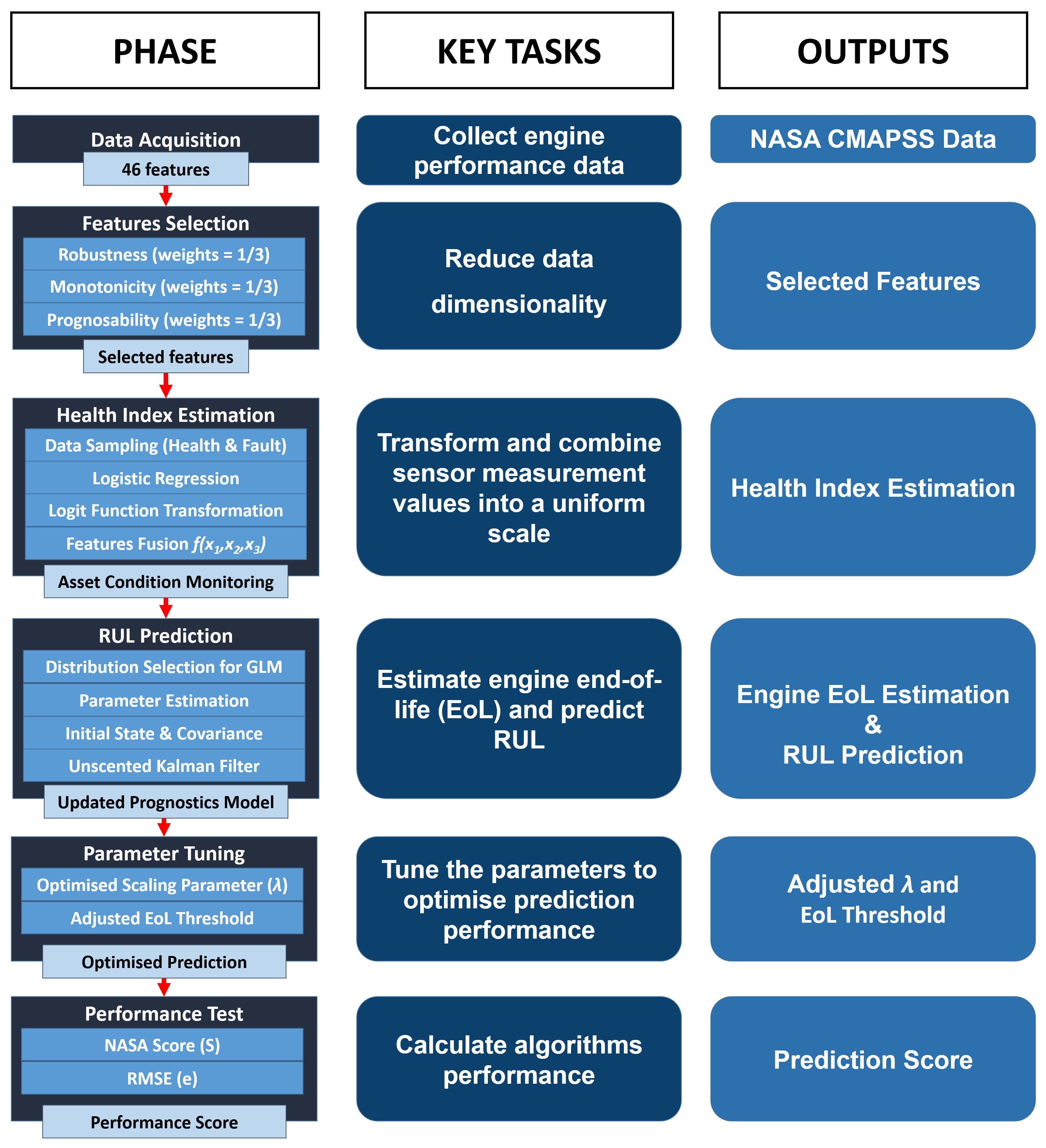
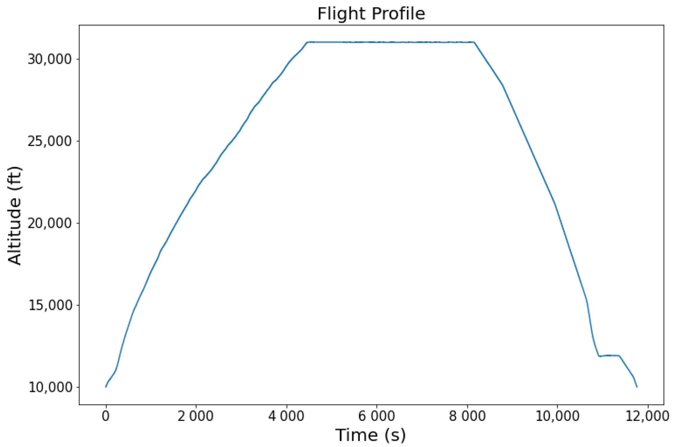
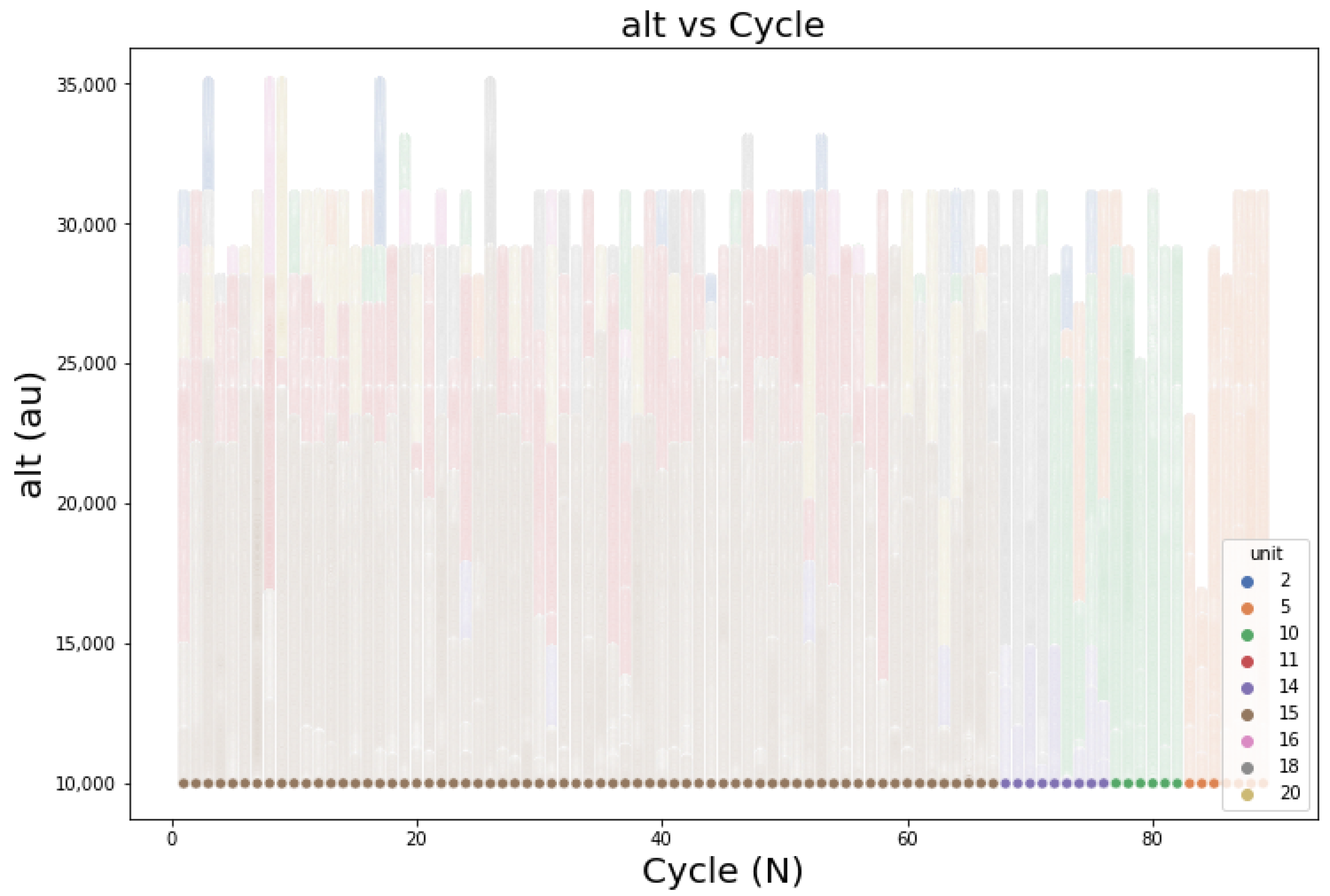
From the Data Acquisition, it is found that the chosen dataset comprises 46 parameters, including scenario descriptor, measurement, real EoL, and model health parameters. Some of the parameters recorded in this dataset are altitude and fuel flow. It is shown in Figure 5 how the aircraft altitude changes over time. The increasing altitude from 10,000 to 30,000 ft occurs in the early flight phase. The steady altitude is maintained for more than 1 h. The height steadily decreased and held for a while before returning to 10,000 ft.

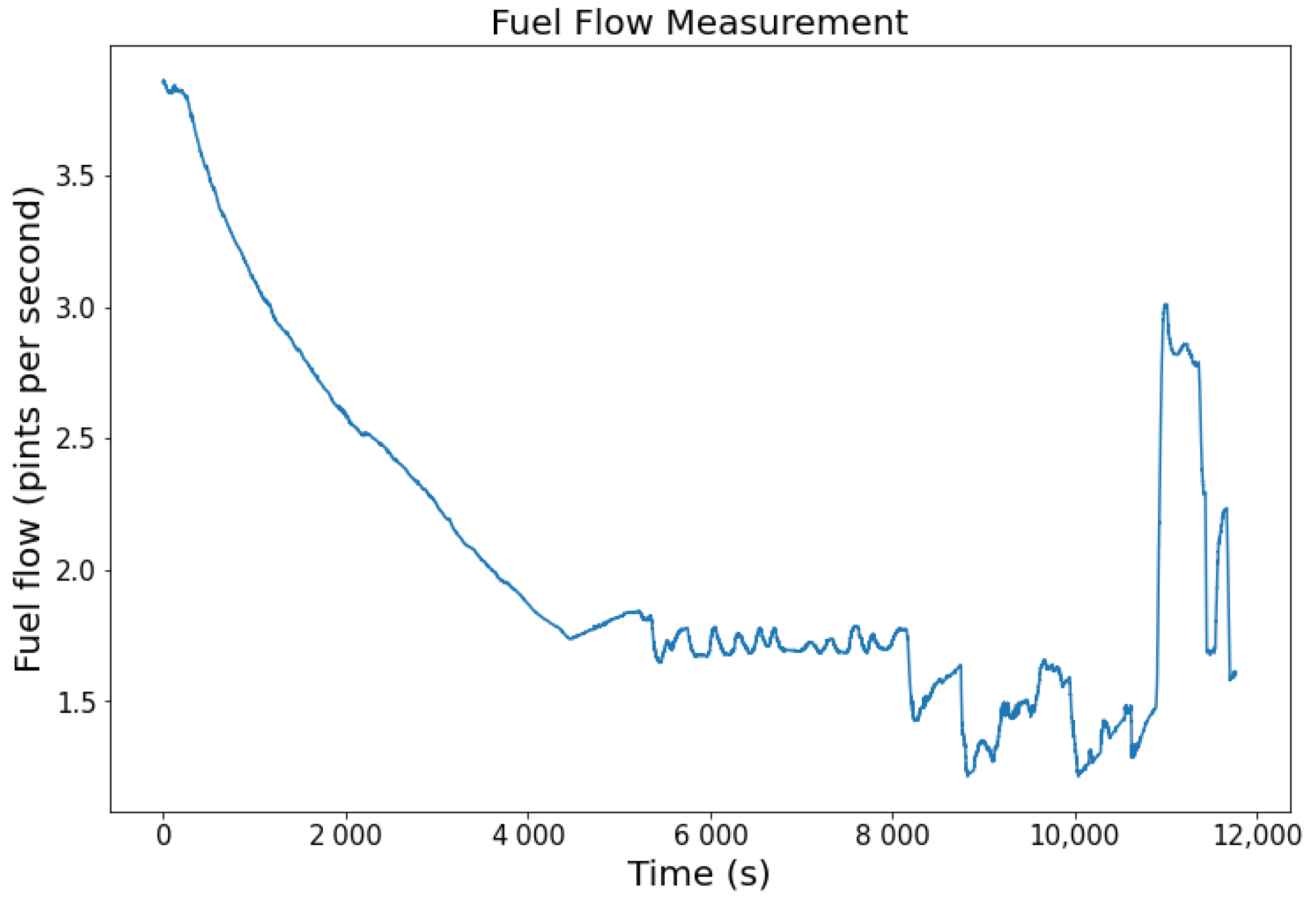
The second example is the fuel flow record as seen in Figure 6. In the early phase, the fuel flow starts at 3.5 pps before rapid degradation is detected. Small fluctuations in the middle sector happen for more than 4000 s. As it approaches the end of the flight, the fuel flow exhibits high volatility, where its highest peak is 3 pps before instantaneously dropping at the end.

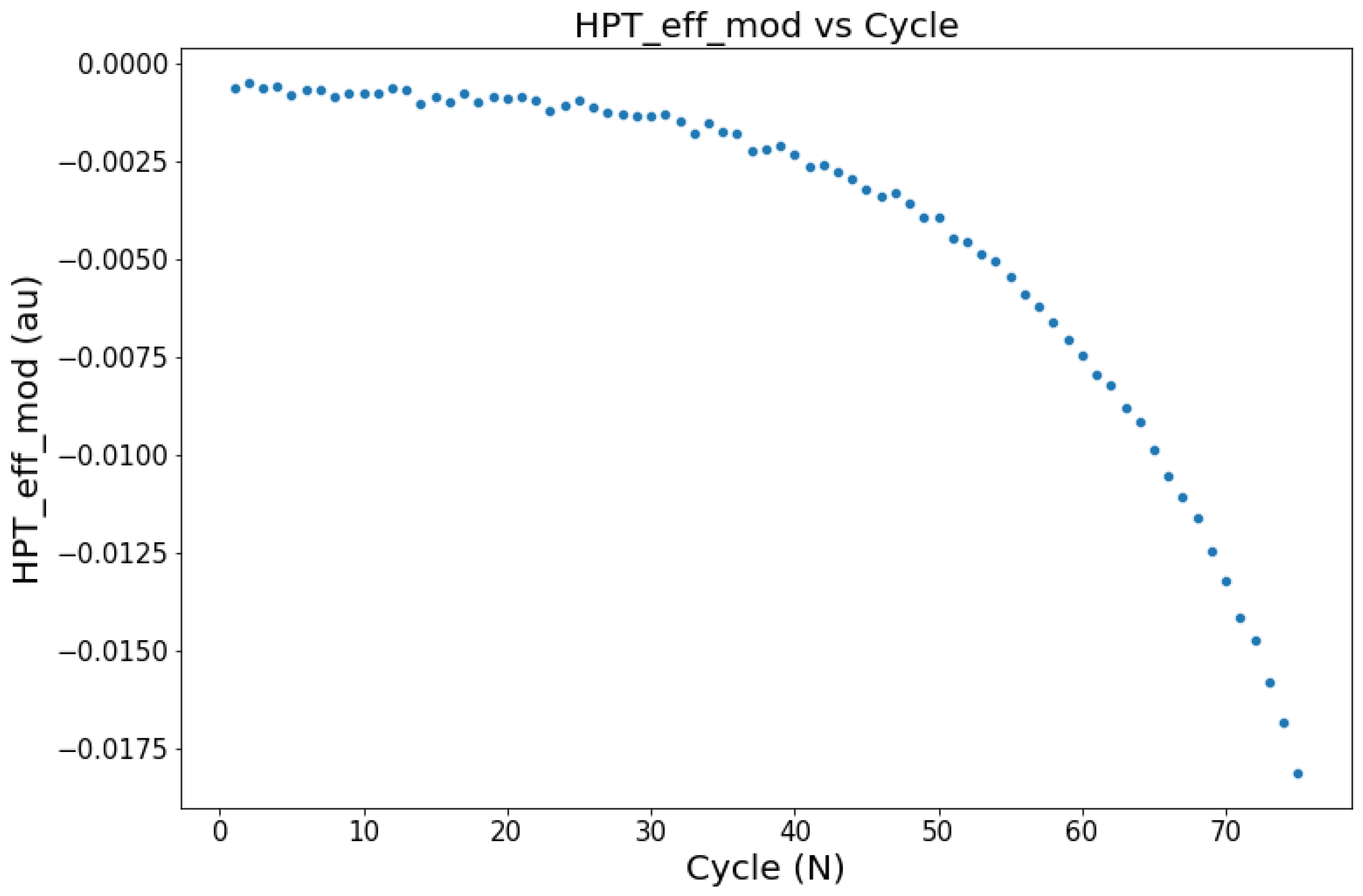
Following the flight altitude (see Figure 5), the fuel flow parameter of the same aircraft (Figure 6) is a match for the same flight. The high fuel flow at the beginning shows that the aircraft requires high power during the take-off and climb phase. The fuel flow becomes steady during the cruise. In the descend and landing phases, the fuel flow fluctuated depending on the pilot’s demand to maintain or decrease the altitude. This synchronicity between these two parameters shows that the CMAPSS data approximate the real flight condition. Furthermore, sub-system degradation can be monitored in each cycle until it fails. For instance, degradation in $HPT\_eff\_mod$ in Figure 7 may occur on a real system due to operating conditions. These factors are ideal to build a model that approximates the real flight condition.

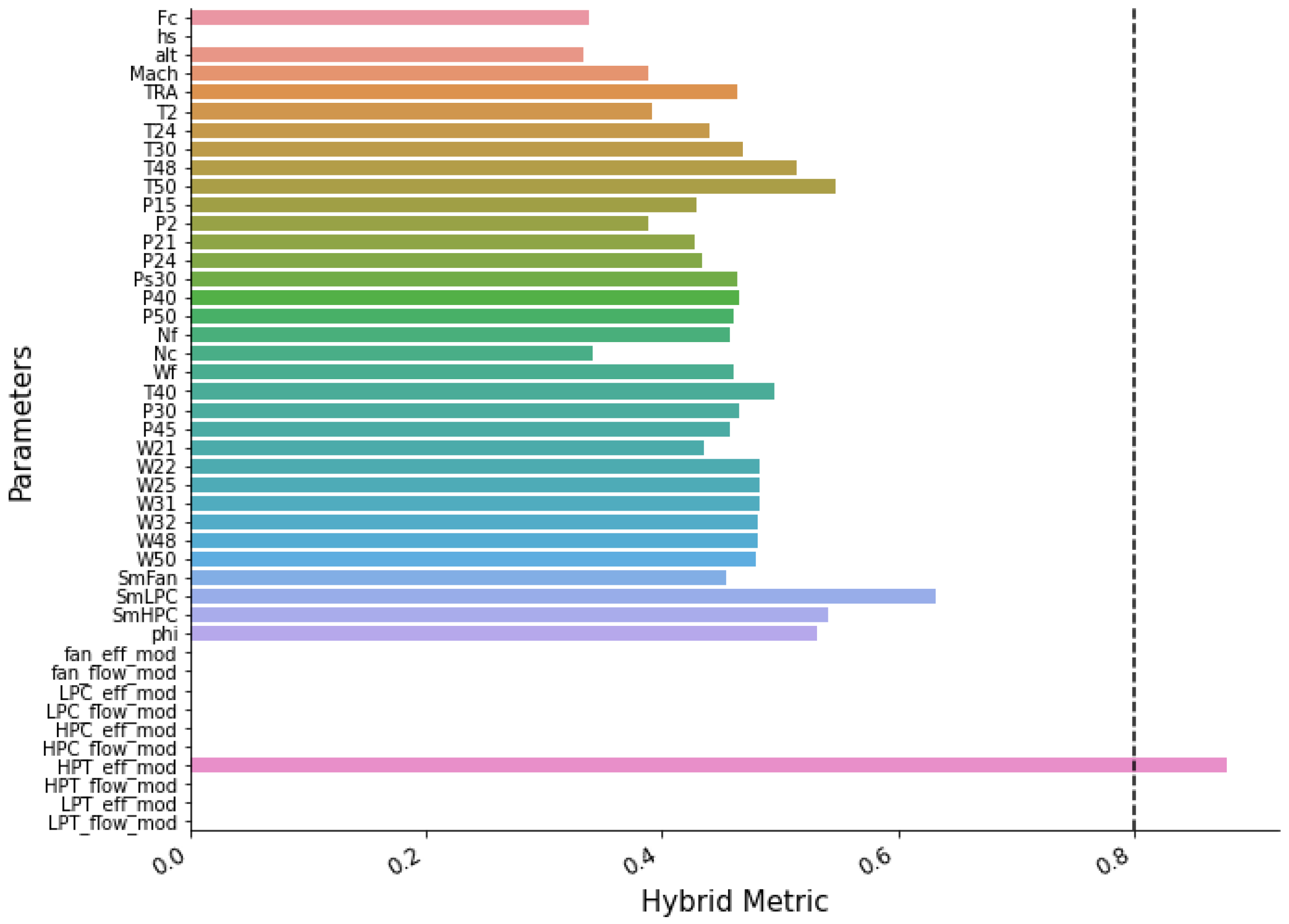
All features from DS02 and DS03 are passed through the hybrid metrics in the Feature Selection phase. A threshold is assigned, and only feature(s) that have a metric score above the threshold will be the selected feature. The 0.8 metric value is set as the threshold since it is a high enough value to filter a good feature but not too high where none will pass.

Figure 8 presents the result of the hybrid filtering of DS02. It shows that $HPT\_eff\_mod$ has the highest metric score (0.87) and is the only feature that passes the threshold. It is noted that several features show metric scores of 0, such as the fan efficiency modifier ($fan\_eff\_mod$) and low-pressure turbine (LPT) efficiency modifier ($LPT\_eff\_mod$). Altitude is the feature with a non-zero and the lowest metric score with 0.33.

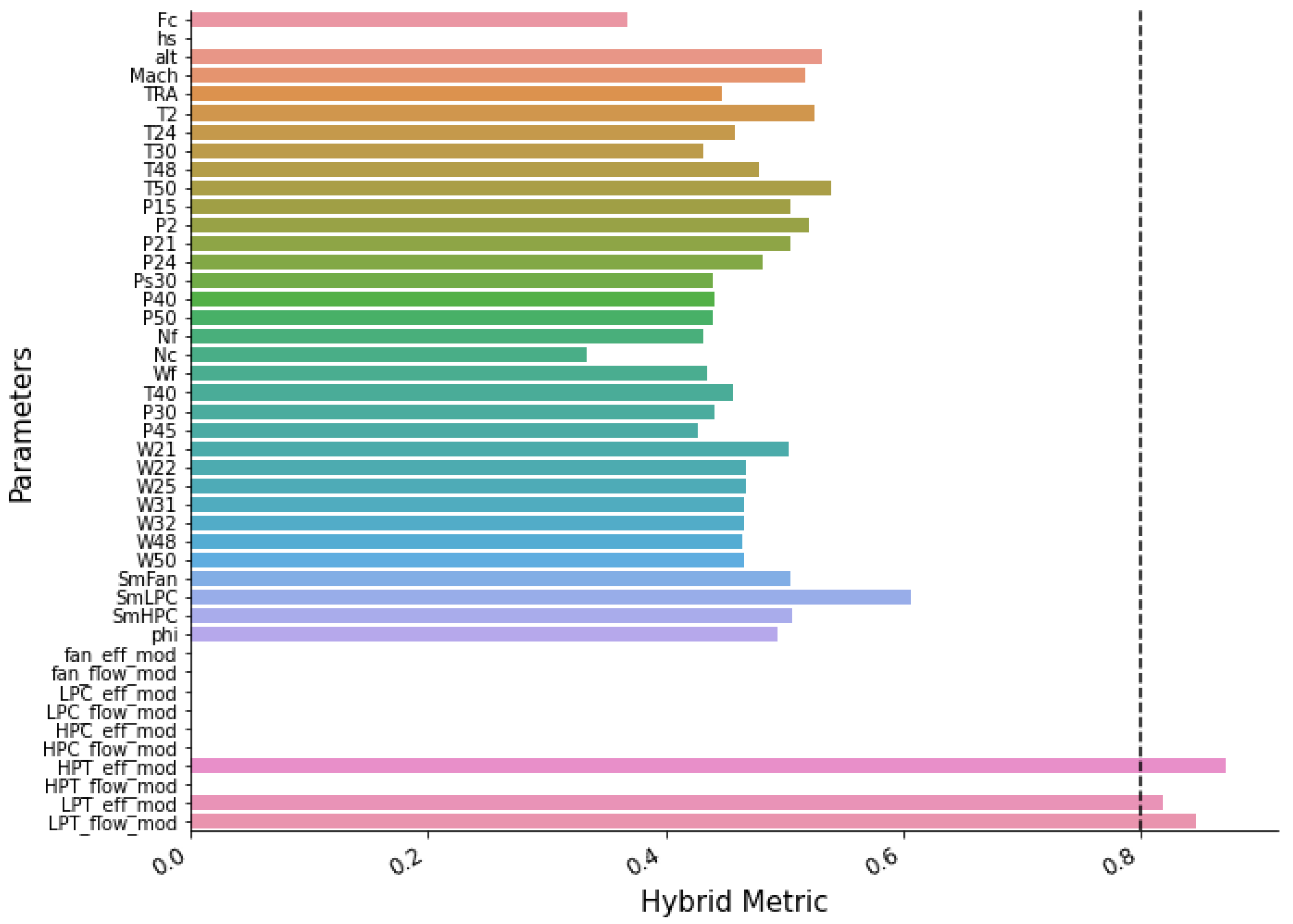
The filtering of DS03 exhibits a different result, as shown in Figure 9. These three features pass the filtering process, namely $HPT\_eff\_mod$, $LPT\_eff\_mod$, and LPT flow modifier ($LPT\_flow\_mod$). These features yield high metric scores with $HPT\_eff\_mod$ as the highest (0.87) followed by $LPT\_flow\_mod$ (0.84) and $LPT\_eff\_mod$ (0.81). Like in the DS02, several parameters show a 0 metric score. The lowest score and non-zero feature is physical core speed (Nc), with a 0.33 metric score.

In the Health Index Estimation phase, the data sampling from the selected features is performed to check the measurement values when the engine is in a healthy ($F_{healthy}$) and failed ($F_{failure}$) state. The tables in Appendix A show the example of sampling data from DS02 (

Table A1. Data sampling healthy state (DS02).

Engines	Fhealthy
	HPT_eff_mod
2	−0.0006375
	−0.0004876
	−0.0006266
	−0.0005803
	−0.000823
5	−0.0007052
	−0.000683
	−0.0008893
	−0.001015
	−0.000755

and

Table A2. Data sampling failed state (DS02).

Engine	Ffailure
	HPT_eff_mod
2	−0.01415
	−0.01475
	−0.01581
	−0.01685
	−0.01814
5	−0.01496
	−0.01593
	−0.01668
	−0.0175
	−0.01866

) and DS03 (

Table A3. Data sampling healthy state (DS03).

Engine	Fhealthy
	HPT_eff_mod	LPT_eff_mod	LPT_flow_mod
1	−0.0004163	−0.0002074	−0.000945
	−0.0002801	−0.0002935	−0.0008464
	−0.0004916	−0.0002692	−0.000682
	−0.000327	−0.0003037	−0.000674
	−0.0002173	−0.0003734	−0.001058
2	−0.000459	−0.0001724	−0.0002406
	−0.0005145	−0.0004094	−0.0000645
	−0.000308	−0.0003061	−0.0002099
	−0.000374	−0.0004992	−0.0002725
	−0.0006175	−0.0002141	−0.00007236

and

Table A4. Data sampling failed state (DS03).

Engine	Ffailure
	HPT_eff_mod	LPT_eff_mod	LPT_flow_mod
1	−0.002703	−0.003067	−0.01602
	−0.00282	−0.00333	−0.01733
	−0.002947	−0.00333	−0.01915
	−0.00303	-0.003426	-0.02199
	−0.003298	−0.003448	−0.0239
2	−0.005596	−0.00593	−0.01662
	−0.005775	−0.006138	−0.01773
	−0.006004	−0.006844	−0.01917
	−0.006245	−0.00732	−0.02055
	−0.006706	−0.00762	−0.02234

). Five measurements of $F_{healthy}$ and $F_{failure}$ of the selected features are taken across the engine fleet. As seen in the tables, the value and range of the features are different even if they represent the same state (healthy or failed state).

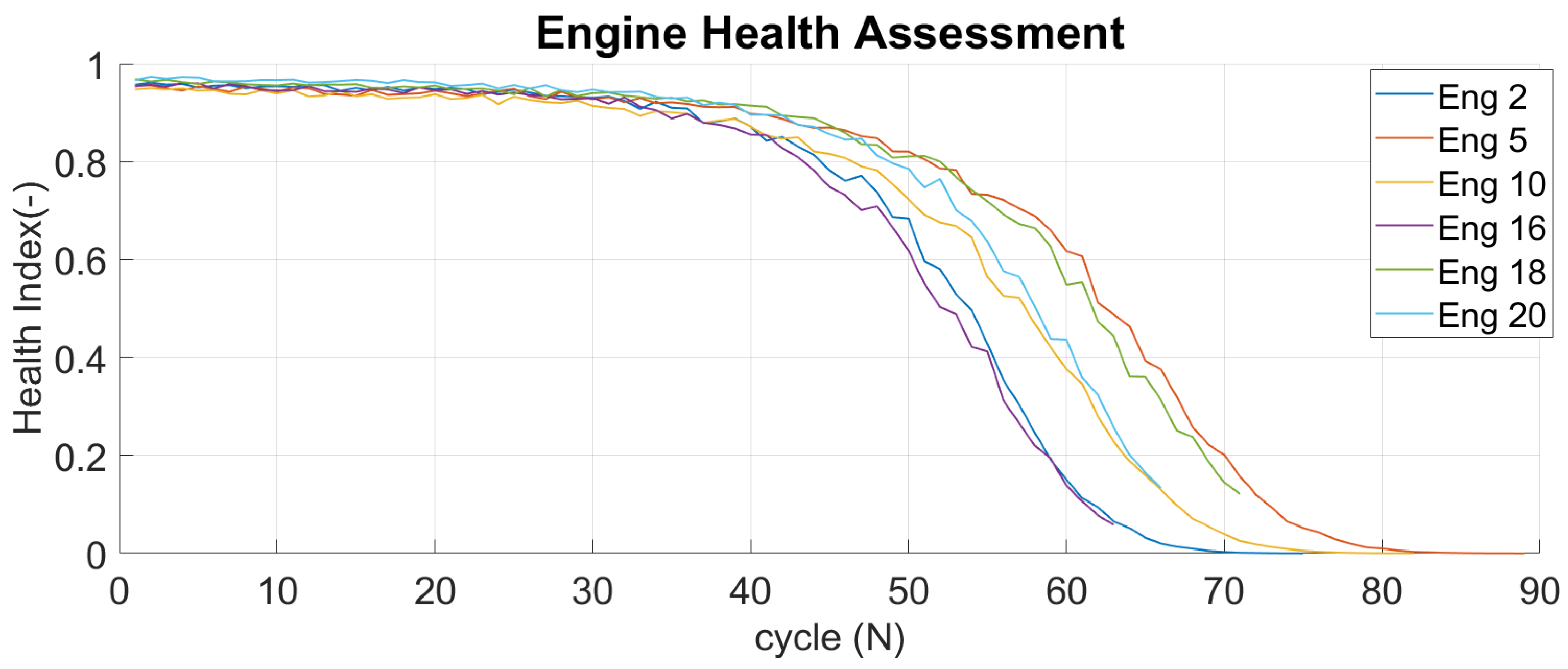
This sample data is then used for logistic regression to obtain function parameters. The computed parameters of each engine are employed to identify the health index (HI) from measurement data. Figure 10 compares HI from across the fleet of DS02. Similarly, Figure 11 provides the same comparison for DS03 and it also shows the strict HI range from 1 (healthy) and 0 (failed). Although both datasets show the same pattern across the fleet, each unit has a unique and distinctive degradation rate. Since each engine has different parameter values, the HI becomes a measure of the engine’s health for engine condition monitoring process.

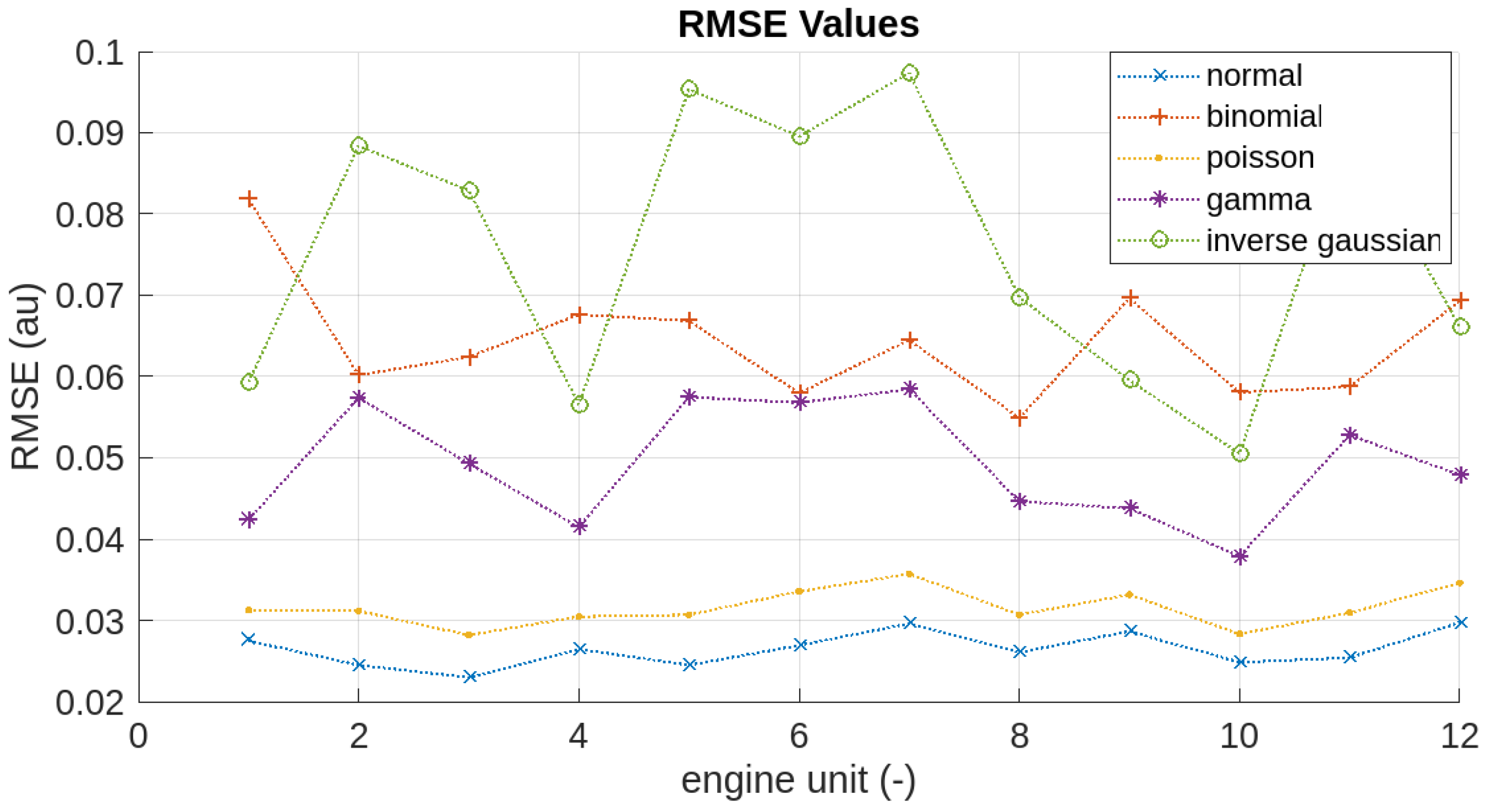
The distribution selection of the response variable (engine HI) is evaluated by calculating the RMSE value in the RUL Prediction phase. Figure 12 is the result of the RMSE plotting across the engine fleet of DS02. RMSE values are collectively highest for engine 10 and lowest for engine 20. Inverse Gaussian and Gamma distributions have relatively high fluctuation, while Binomial, Poisson, and Normal distributions are steadier in all engines. Compared to others, Normal distribution consistently results in the fleet’s lowest RMSE value.

RMSE plotting of DS03 is shown in Figure 13. Higher volatility is seen in DS03 compared to DS02. Inverse Gaussian, Binomial, and Gamma distributions have distinct peaks and bottom differences across the fleet. Even though fluctuate, Poisson and Normal distributions show less peak-bottom difference variance. Similar to DS02, the Normal distribution shows the lowest RMSE for this dataset. Hence, both datasets use the Normal distribution for GLM fitting process.

The GLM fitting with logistic regression transforms these sampling data and results in each engine’s logit function ($\alpha$ and $\beta$) parameters.

Table A5. Logit Function Parameters of DS02.

Engine	$\mathit{\alpha }$	$\mathit{\beta }$
2	9.9798	−0.19011
5	9.1388	−0.14872
10	8.493	−0.15226
16	8.56975	−0.166061
18	8.29255	−0.136379
20	8.99486	−0.156457

(see Appendix B) provides these parameters of DS02 for each engine. The same process goes for DS03, resulting in different values of logit function parameters that are shown in

Table A6. Logit Function Parameters of DS03.

Engine	$\mathit{\alpha }$	$\mathit{\beta }$
1	23.6247	−0.362276
2	18.0867	−0.293683
3	20.8985	−0.365551
4	18.1902	−0.343259
5	19.8858	−0.250735
6	14.836	−0.285327
7	14.8642	−0.22494
8	14.1709	−0.239175
9	17.8039	−0.243792
10	15.7609	−0.27589
11	15.7065	−0.319659
12	15.8	−0.198393

in Appendix B.

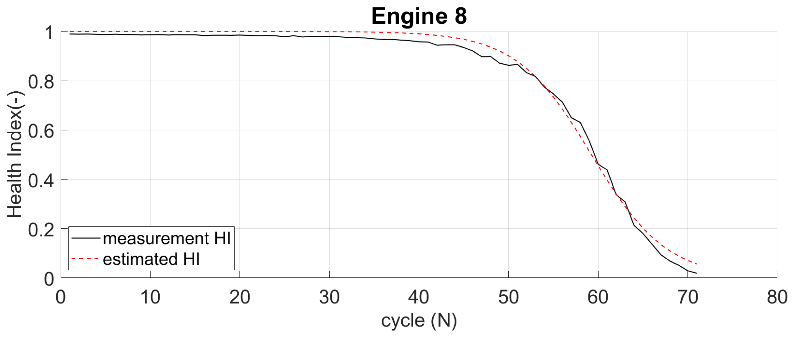
The computed parameters of each engine are then used to identify the estimated health index (HI). Figure 14 compares HI from measurement and estimated HI from the logistic regression of engine 16 (DS02). Similarly, Figure 15 provides the same comparison for engine 8 (DS03). The HI from measurement begins near 1 (but not at 1), while the estimated HI always starts at 1 (100% healthy). Even though there is a slight difference, both show the engine in a healthy state at the beginning. Both end almost at the same values when the aircraft is in a failed state.

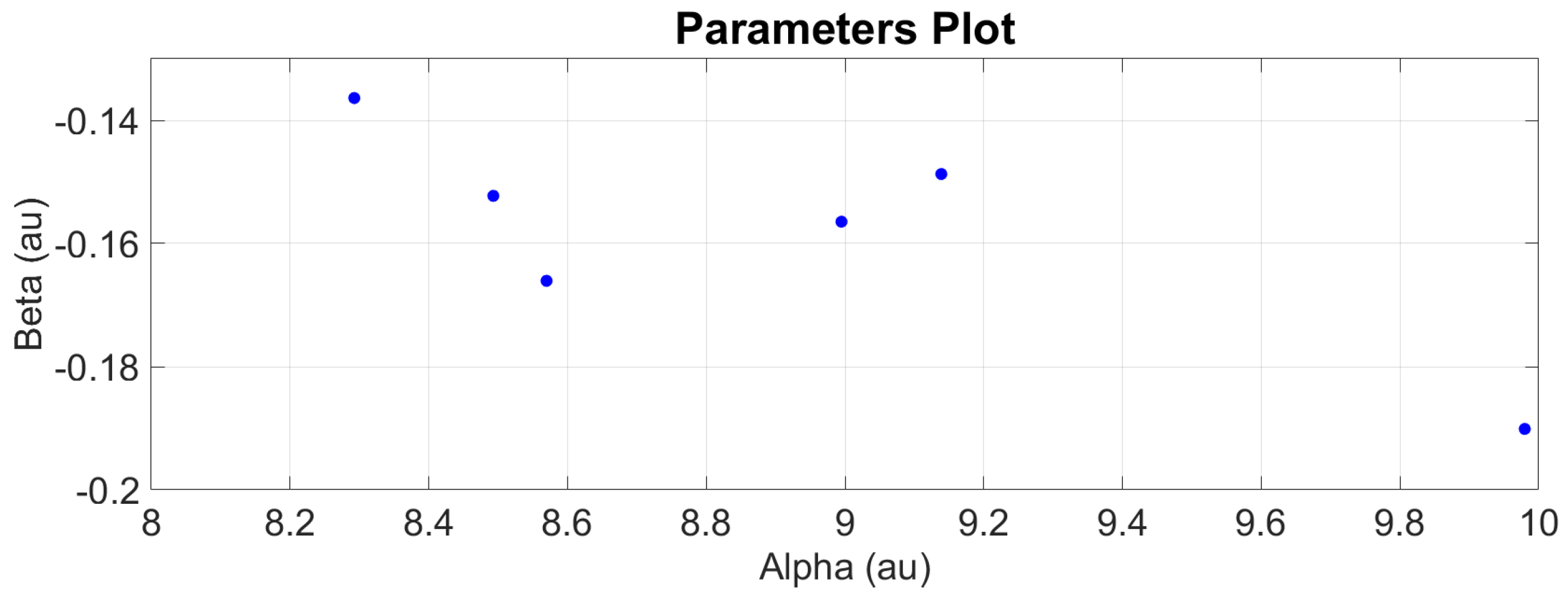
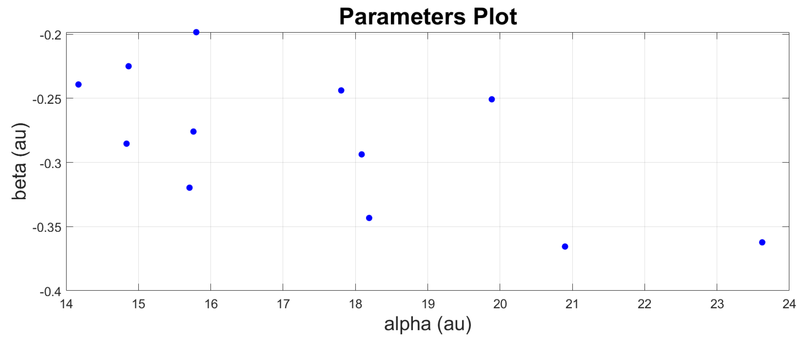
The parameters of each engine are then plotted against each other to identify their scatter points. Figure 16 and Figure 17 show how the parameters are distributed. It follows no pattern and is randomly distributed. The mean values of $\alpha$ and $\beta$ are computed to represent the fleet parameters. The covariance is also computed to show how much alpha and beta vary together. The mean values and covariance matrix are then set as the initial state ($X_0^{+}$, $P_0^{+}$) for the unscented Kalman filter (UKF) process.

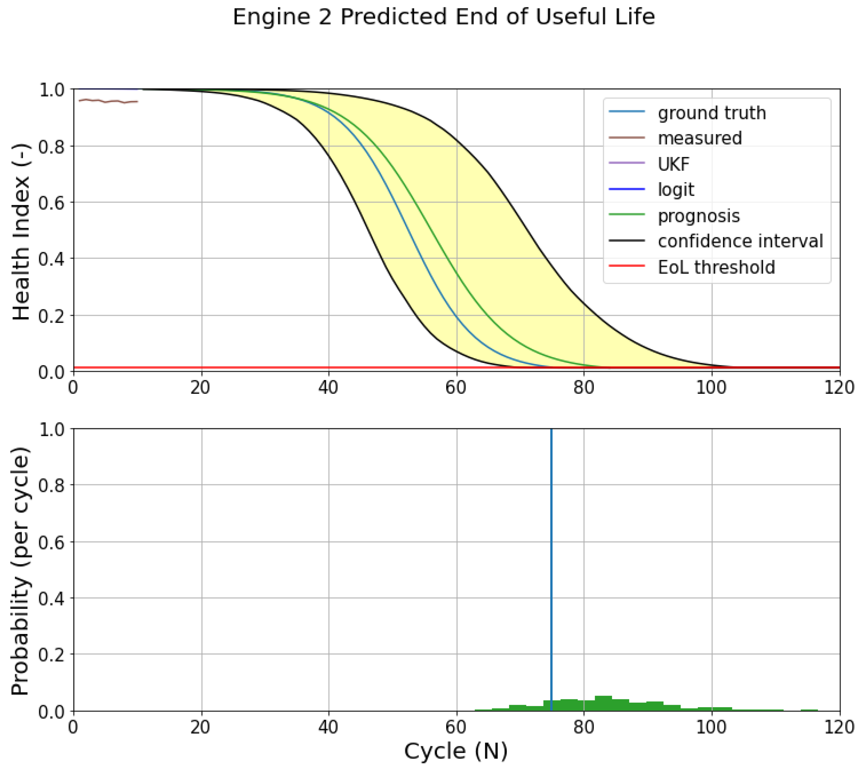
After estimating the engine system state, the UKF produces new (updated) parameters (${\alpha }_k$ and ${\beta }_k$). The extrapolation of the logit function is computed based on these new parameters. Figure 18 shows the engine end-of-life (EoL) and RUL distribution based on 1000 trajectory samples.

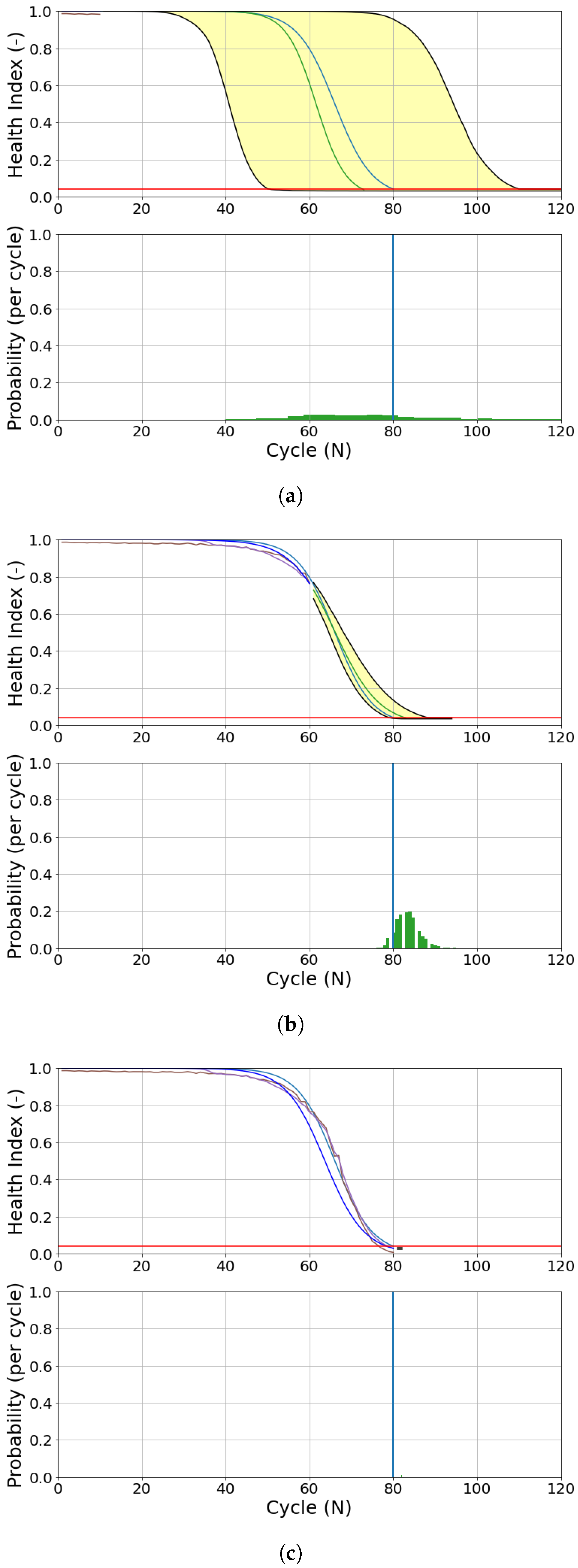
As a result of the recursive update in UKF, the parameters are updated in each cycle, producing a new (updated) prognostics model. This updated model extrapolates 1000 possible trajectories and estimates engine end-of-life (EoL) and RUL probability distribution. As seen in Figure 19 for Engine 2 (DS02), the prediction starts when there is information from measurement data (sensors). In the first 10 cycles, the EoL estimation has a poor performance, shown by a large 90%-confidence interval area (yellow-shaded area). The RUL prediction maps the probability distribution of these possible EOLs and still has a low probability value in the early flights (measurement).

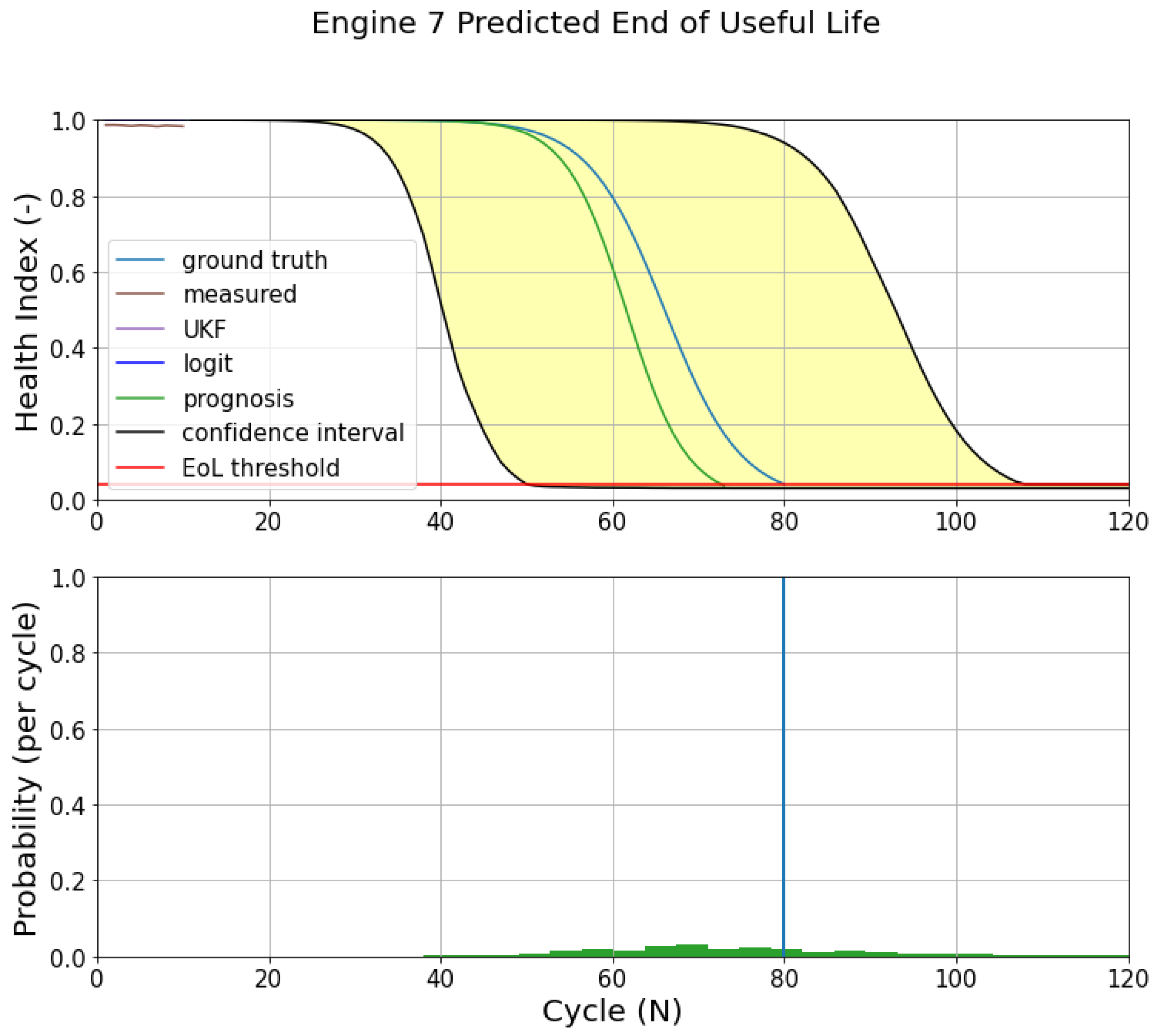
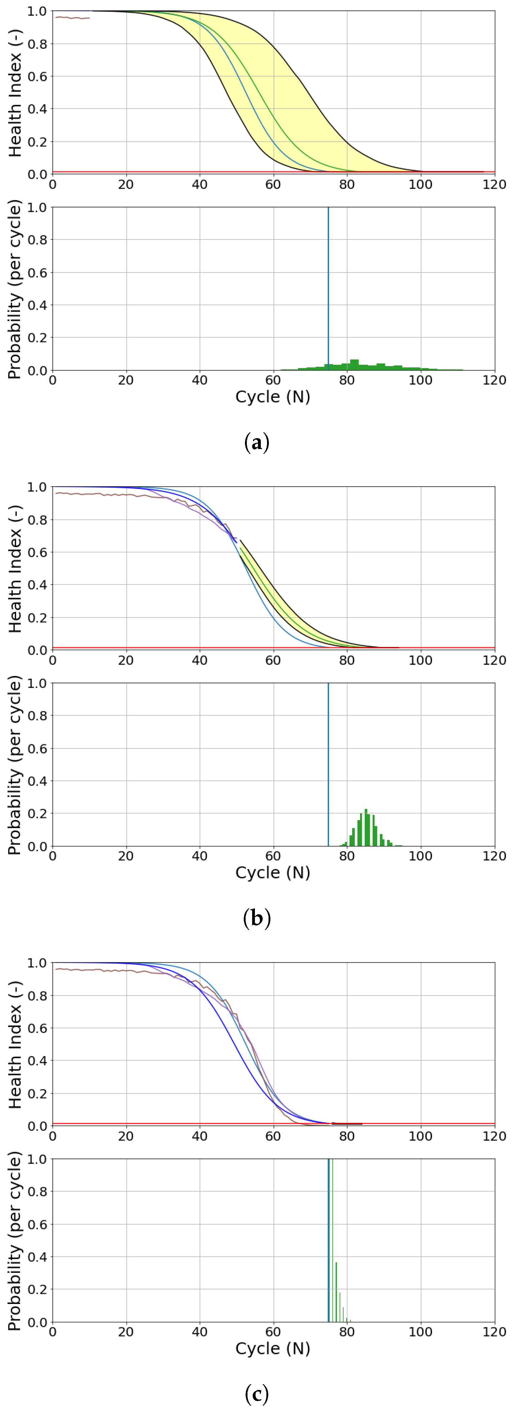
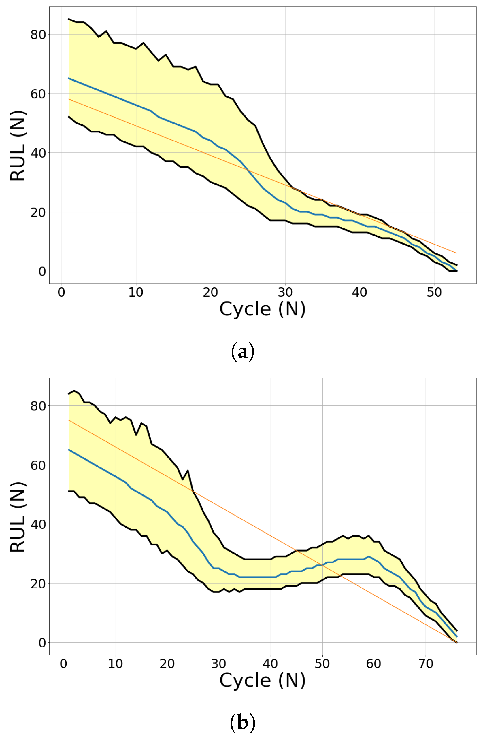
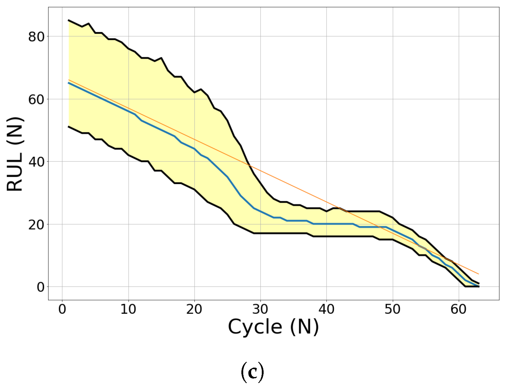
Like DS02, similar phenomena are also observed in DS03. Figure 20 shows the prognostics model of engine 7 (DS03). The initial measurements (10 cycles) present a sub-optimal prediction. On the following flights (60 and 80 cycles), the updated prognostics model has a better prediction, as shown in Figure 21c. Both EoL and RUL predictions converge around the ground truth EoL (80 cycles).

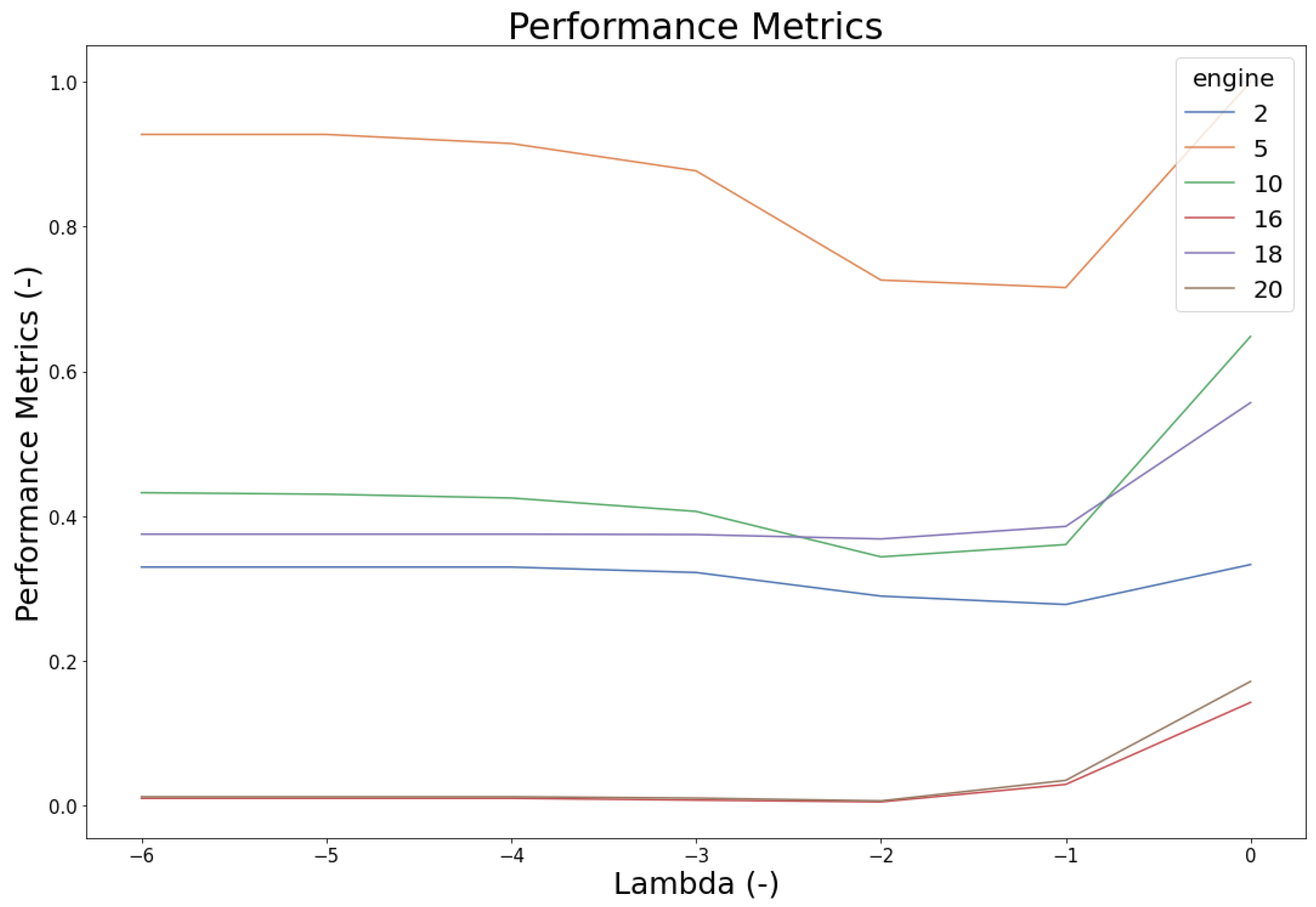
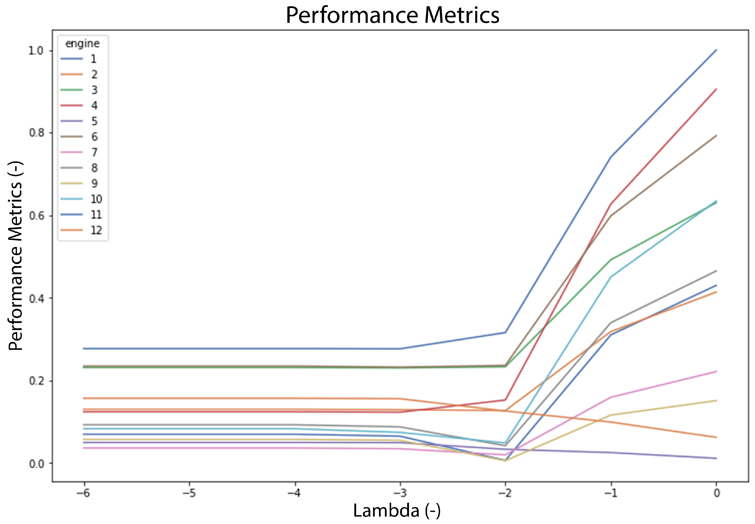
The Parameter Tuning phase attempts to find the optimised parameter in order to obtain the best prediction result. Once the base model has been set up, the scaling parameter ($\lambda$) and EoL threshold are tuned and the prediction results are presented in performance metric (p). Figure 22 and Figure 23 show that $\lambda$ value $1\times {10}^{-2}$ yields the collective optimal result for both datasets. As for the EoL threshold, several approaches are explored by using mean, max, and SPC (with 1$\sigma$, 2$\sigma$, and 3$\sigma$) value of the EoL from the training engines. 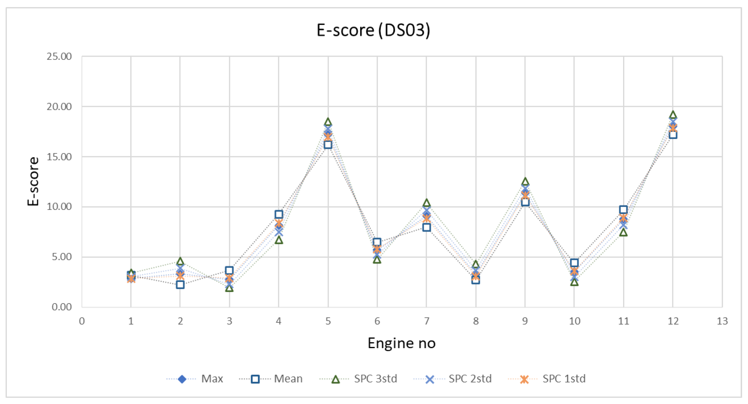Figure 24 and Figure 25 are the example of the EoL tuning process of DS03 by comparing s and e score of each method. From these figures, mean and SPC 1$\sigma$ show a good prediction performance. Even though the mean value provides good results, but the SPC 1$\sigma$ shows optimum performance fleet-wise. Hence, the SPC 1$\sigma$ value of EoL from the training engines will be the threshold.

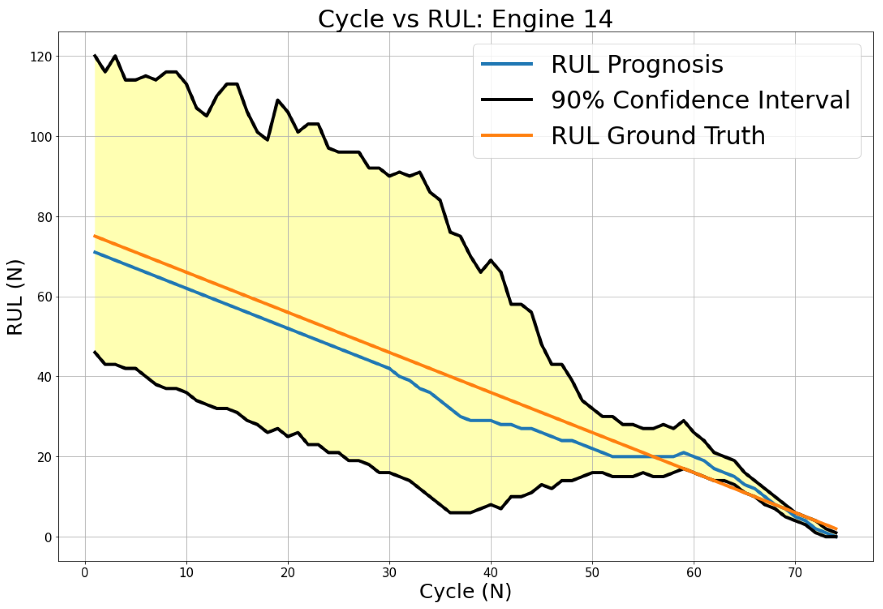
The result of the optimised model from the training dataset is put into assessment in the Performance Test phase. The test engine dataset becomes the input of the trained algorithms. The evaluation metrics are computed against the prediction result of this test dataset. Figure 26 shows the sample of the algorithm RUL prediction performance on test engine 14 (DS03). The predicted RUL is plotted and compared to the ground-truth RUL. Figure 27 and Figure 28 present visual information of how the prediction progresses over time for DS02 and DS03, respectively. The prediction performance on both datasets results in a high uncertainty (yellow-shaded area) at the early flight, but it decreases as the engine approaches the EoL. The RUL from the prognostics model fluctuates around ground-truth RUL, and it is noted that most of the predictions end under the ground truth. In comparison to DS02, the predicted RUL of DS03 is steadier relative to the ground truth, but it has a higher uncertainty level before rapidly decreasing toward the EoL.

The quantification of the performance on the test dataset is presented as e and s scores. As mentioned in Section 2.6, these evaluation metrics are standard and comparable since they are widely used in this research area.

Table 2. Evaluation metrics of the test engines with the proposed method.

Dataset	Engine	s	e
DS02	11	91.29	5.1
	14	196.91	11.9
	15	97.7	5.84
DS03	13	126.74	6.8
	14	109.72	5.1
	15	87.26	3.04

provides the s and e scores of DS02 test engines (11,14, and 15) and DS03 Engines (13,14,15). Engine 11 (DS02) and engine 15 (DS03) retain the lowest with 91.29 and 87.26 for the s score and 5.1 and 3.04 for the e score for both engines, respectively. Slightly higher values are shown in engine 15 of DS02 with 97.7 (s score) and 5.84 (e score), while engine 14 of DS03 acquires 109.72 s score and 5.1 e score. Lastly, engine 14 has the highest score among DS02 with a s score of 196.91 and e score of 11.9. Similarly, engine 13 presents a 126.74 s score and 6.8 e score; both are the highest in DS03.

3.2. Discussions

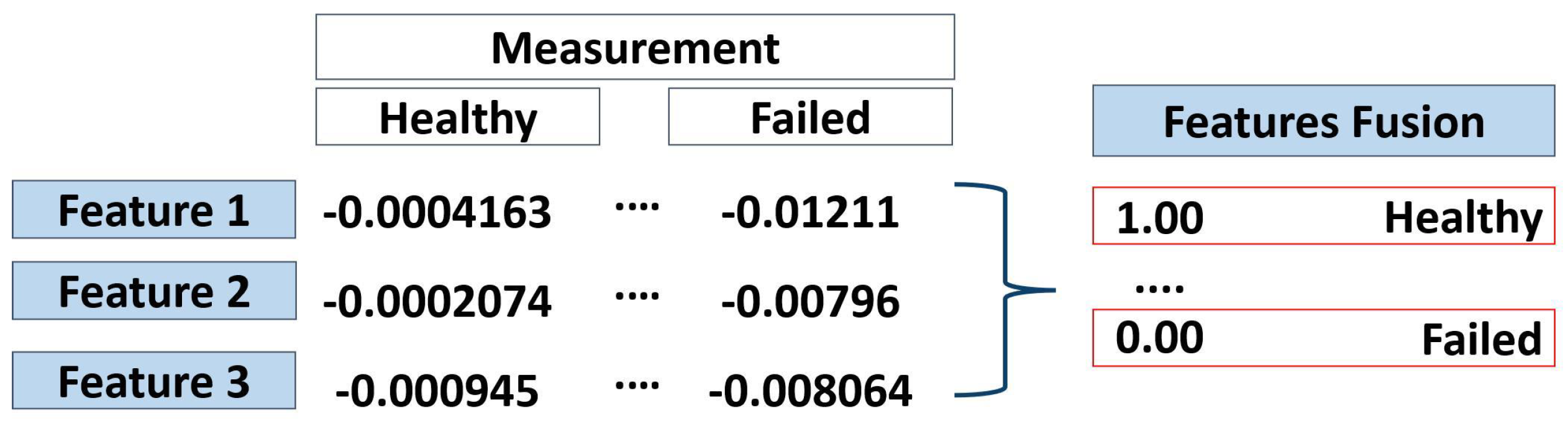
In the Features Selection phase, the hybrid filter effectively chooses the critical features for both DS02 and DS03. Figure 29 is an example of a selected feature from DS02 and, like all selected features, it fulfills all criteria: robust, monotony, and prognosable. On the other hand, features with the worst metric value show a random pattern and are difficult to interpret (see Figure 30). However, the filtered features from the sensors are still arbitrary, and it has little to no direct interpretable information (see Figure 3). Hence, feature fusion and health index estimation are necessary to address this issue.

The results of Health Index Estimation are shown by health index (HI) value, ranging from 0 to 1 (0–100%). The logistic regression computes the function parameters that influence the HI value of each engine. The effects of these parameters are visually shown in both Figure 10 and Figure 11. The parameters ($\alpha$ and $\beta$) determine the engine’s health intercept and degradation rate, respectively. The lower the $\beta$, the faster the engine degrades. Since each engine has a different parameter value and shows a unique pattern, the HI is suitable for measuring the engine’s health for the individual condition monitoring process. Hence, the condition-based maintenance (CBM) strategy can be developed around this information.

The advantages of the proposed technique in condition monitoring applications are:

• It requires less training data.
  This approach only needs five samples of engine healthy state $F_{healthy}$ and five samples from failed state $F_{failure}$. It is convenient if the available data is limited while maintaining a good approximation of asset conditions.
• Intuitive HI.
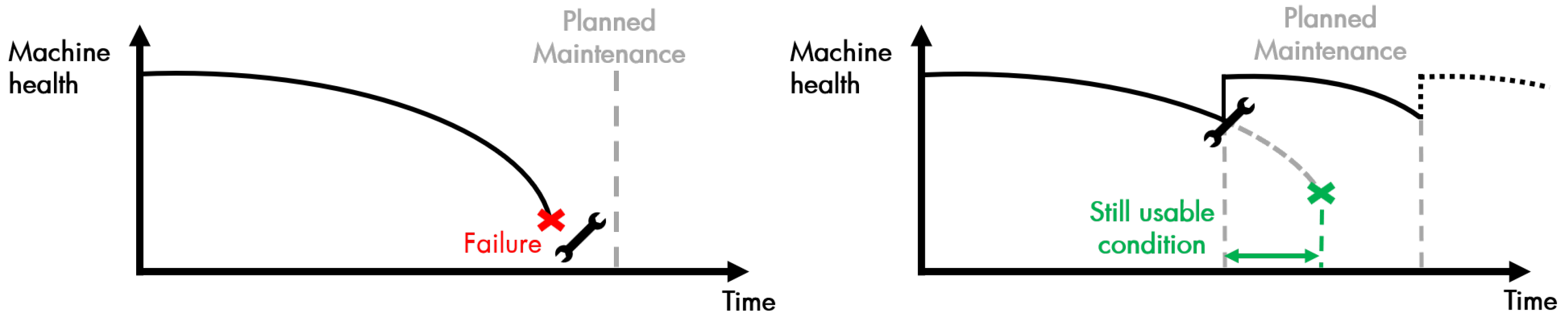
  The engine health condition is represented by a finite range of 0 to 1. This range can mean the level of engine healthiness where 0% is a complete failure and 100% means the engine is in a brand-new condition. The value between 0 and 100% offers more intuitive and meaningful information to the operator compared to the current approach that relies on prescribed intervals without knowing the reliability level of the engine (see Section 1.1). With these finite values, a threshold(s) can be determined based on their experience or other consideration. For instance, the operator can start planning for a shop visit when the engine reliability level is at 25% or below.
• It provides discrete HI information across the engine fleet.
  As discussed in Section 1.1, the downside of the current practice is only focusing on fleet-wise and lacks individual engine assessment. This paper offers a distinctive HI from measurement data of every single engine in DS02 and DS03. Individual health assessment means the maintenance schedule is tailored to each engine’s current condition rather than a fixed schedule.
• It shows the engine degradation process.
  In order to build a prognostics system, asset degradation must be clearly identified. This CBM process is part of prognostics phase where engine degradation detection and pattern recognition processes occur. Information from the CBM process will then be used in the next process of prognostics development.

However, despite the advantages, this paper does not cover all properties of PHM, such as:

• Anomaly and fault detection are not included in the process.
  Despite the necessity of this detection process for warning, it is not covered in this paper’s scope Section 1.3. The NASA CMAPSS datasets do not explicitly provide this information, and further analysis is required to generate the anomaly and fault detection system. Thus, further research can explore this opportunity to create a more comprehensive approach.
• Failure mode of the component is not provided.
  Although this technique can identify the engine’s degradation and fault, the failure mode of the failed sub-system (or component) is not considered. The main rotating engine sub-components (fan, LPC, HPC, HPT, and LPT) show a continuous degradation process in this simulated dataset [19]. However, this paper focuses on the engine as the whole system rather than individual sub-system failure.

A Filtering-based model is chosen for prognostics in RUL Prediction phase due to its suitability in estimating a joint state of the asset [18]. The UKF updates the function parameters ${\alpha }_k$ and ${\beta }_k$ based on a recursive process. These parameters are then used to extrapolate the prognostics model (green line) and predict engine EoL against the threshold (red line) (see Figure 18).

Uncertainty Quantification (UQ) is shown by a yellow-shaded area representing a 90% confidence interval. Another UQ is shown by the probability distribution of RUL in the lower part of the same figure. As expected, the uncertainty decreases over time, as shown by the reduced yellow-shaded area and the increasing probability distribution around ground truth (blue line).

This approach provides several benefits, especially in prognostics applications, such as:

• Provides a high level of transparency.
  All computations and processes are visible and known in this research. This feature offers the operator a flexible and agile tool to produce an optimised result. In the Parameter Tuning phase, it is shown by adjusting the $\lambda$ (scaling parameter) and EoL threshold (see Section 2.5 and Section 3.1) can optimise the prediction result. Since the process is transparent, diagnosing the algorithm is easier if there is any inaccuracy in the prediction compared to the “black box” process (such as the machine learning approach). It is important to note that this characteristic is one of the highlights of this paper to tackle the discussed research gap (see Section 1.3).
• Uncertainty is clearly quantified.
  As stated in Section 1.3 and [25], one of the most significant barriers to prognostics application in the industry is the lack of uncertainty quantification. This paper addresses this issue by computing all possible prediction outcomes with a 90% confidence interval. Figure 27 and Figure 28 show the uncertainty in the RUL prediction of DS02 and DS03 consecutively. This information is critical for the operator since it can improve confidence in the maintenance decision-making process and estimate the possible outcomes.
• Requires fewer data.
  This approach only selects the critical parameter(s) and uses fewer data points to train the algorithms. The UKF uses a recursive process where the prediction can be autonomously computed once measurement data is available and the operating time increases. This approach is suitable for a real scenario where the recorded and “run-to-fail” data are limited (see Section 1.1).

As seen in Figure 27 and Figure 28, the RUL predictions are mostly lower than the ground truth. Hence, it does not accurately predict the real RUL. However, it is intentional, by adjusting $\lambda$ and threshold, and convenient since it is preferable to predict early rather than later, considering the safety-critical nature of the aircraft engine. Significant uncertainty in the test engine of DS03 is another drawback of this algorithm, especially in the early to middle sector. Even though it significantly decrease in the last sector, it is still challenging to determine the appropriate maintenance intervention. Future research may benefit from exploring a way to reduce this uncertainty, especially in the early flights, which can improve prediction performance.

The results from the Performance Test phase were then compared to previous works. Among three previous works that used the latest CMAPSS data, only [24] uses the same test engine and same evaluation metrics as this research.

Table 3. Performance comparison between the method proposed in this paper and the previous work (*) [24].

Engine	s	s *	e	e *
11	91.29	130	5.1	11.49
14	196.91	114	11.9	10.91
15	97.7	82	5.84	8.92

shows the evaluation metrics of the previous finding [24] compared to this research.

The s score comparison shows that the proposed method performs better only for Engine 11 with a 91.29 score. While the proposed method accurately predicts RUL with relatively minimum error, it got penalised for overestimating the predicted RUL. The proposed method outperforms the previous work for e score for Engine 11 and 15 with 4.9 and 5.2, respectively. It is important to highlight that the proposed method offers a high level of transparency and uncertainty quantification while keep maintaining a good prediction. Further investigation on the tuning parameters needs to be explored to improve the evaluation metric score.

4. Conclusions and Future Work

4.1. Conclusions

The primary goal of this paper is to provide a framework and algorithms for aircraft engines and prognostics systems. This paper achieved this aim by critically discussing the current prognostics technology methods and developing algorithms and software tools for condition monitoring and prognostic systems.

• The proposed algorithms show good performance compared to the current state-of-the-art in prognostics, specifically in RUL prediction [24]. NASA scoring (s) and RMSE (e) are used as the metrics to check RUL prediction accuracy (see Section 2.6). The widely-used Dataset 02 (DS02) is analysed, and the result is compared to previous work. While, in general, it has a lower s score, it yields better performance for the e score for engines 11 and 15. It also has significant advantages compared to previous research, with better transparency and uncertainty quantification, which lessens the application barrier in the industry.
• This paper has discussed and pointed out the critical improvement in implementing the proposed method. Other than DS02, this paper also explores Dataset 03 (DS03) from the new NASA CMAPPS. To the best of the author’s knowledge, DS03 has not been utilised for prognostics purposes. DS03 provides more engines than DS02; thus, it is an excellent complement to DS02 for developing algorithms and software tools. The developed software tools of condition monitoring and prognostics system produce essential information for the operator in the decision-making process for better planning and optimising asset uptime.

4.2. Future Work

Reflecting on the results, this paper provides several recommendations for future research to improve technical performance.

• While this paper exploits the explicit information in the time-series data, the implicit features are not explored. The correlation between each parameter can show useful information, such as classification, to improve anomaly and fault detection.
• The contribution and failure modes of the sub-system are not considered in this research. A further investigation of the contribution of each sub-system to the engine system might provide a more comprehensive framework.
• As shown in this paper, tuning parameters ($\lambda$ and the EoL threshold) can improve prediction accuracy. It is worth exploring these (or other) parameters and finding the optimal values to enhance the algorithm’s performance.

References

1. Ahmadi, A.; Söderholm, P.; Kumar, U. On aircraft scheduled maintenance program development. J. Qual. Maint. Eng. 2010, 16, 229–255. [Google Scholar]
2. Rehmanjan, U.H. Reliability analysis and maintenance program for airline seats. In Proceedings of the 2017 Annual Reliability and Maintainability Symposium (RAMS), Orlando, FL, USA, 23–26 January 2017; pp. 1–5. [Google Scholar]
3. Eklund, N.H. Prognostics & Health Management. 2009. Available online: https://phmsociety.org/wp-content/uploads/2009/05/Eklund_Diagnostics_TutorialPHM09.pdf (accessed on 12 October 2022).
4. Chen, J.; Zhao, Y.; Xue, X.; Chen, R.; Wu, Y. Data-Driven Health Assessment in a Flight Control System under Uncertain Conditions. Appl. Sci. 2021, 11, 10107. [Google Scholar] [CrossRef]
5. Loutas, T.; Oikonomou, A.; Eleftheroglou, N.; Freeman, F.; Zarouchas, D. Remaining Useful Life Prognosis of Aircraft Brakes. Int. J. Progn. Health Manag. 2022, 13. [Google Scholar] [CrossRef]
6. Ellefsen, A.L.; Æsøy, V.; Ushakov, S.; Zhang, H. A comprehensive survey of prognostics and health management based on deep learning for autonomous ships. IEEE Trans. Reliab. 2019, 68, 720–740. [Google Scholar]
7. Ben-Daya, M.; Kumar, U.; Murthy, D.P. Introduction to Maintenance Engineering: Modelling, Optimization and Management; John Wiley & Sons: Hoboken, NJ, USA, 2016. [Google Scholar]
8. BS EN 13306: 2017; Maintenance—Maintenance Terminology. British Standards Institution: London, UK, 2017.
9. ISO 13381-1:2004; Condition Monitoring and Diagnostics of Machines—Prognostics. Distributed through American National Standards Institute (ANSI): Washington, DC, USA, 2015.
10. Eker, O.F.; Camci, F.; Jennions, I.K. A new hybrid prognostic methodology. Int. J. Progn. Health Manag. 2019, 10. [Google Scholar] [CrossRef]
11. Daigle, M.J.; Goebel, K. Model-based prognostics with concurrent damage progression processes. IEEE Trans. Syst. Man Cybern. Syst. 2012, 43, 535–546. [Google Scholar] [CrossRef]
12. Cubillo, A.; Vermeulen, J.; de la Peña, M.R.; Casanova, I.C.; Perinpanayagam, S. Physics-based integrated vehicle health management system for predicting the remaining useful life of an aircraft planetary gear transmission. Int. J. Struct. Integr. 2017, 8. [Google Scholar] [CrossRef]
13. Heng, A.; Zhang, S.; Tan, A.C.; Mathew, J. Rotating machinery prognostics: State of the art, challenges and opportunities. Mech. Syst. Signal Process. 2009, 23, 724–739. [Google Scholar] [CrossRef]
14. Tsui, K.L.; Chen, N.; Zhou, Q.; Hai, Y.; Wang, W. Prognostics and health management: A review on data driven approaches. Math. Probl. Eng. 2015, 2015, 793161. [Google Scholar]
15. Li, X.; Ding, Q.; Sun, J.Q. Remaining useful life estimation in prognostics using deep convolution neural networks. Reliab. Eng. Syst. Saf. 2018, 172, 1–11. [Google Scholar]
16. Yang, B.S.; Di, X.; Han, T. Random forests classifier for machine fault diagnosis. J. Mech. Sci. Technol. 2008, 22, 1716–1725. [Google Scholar]
17. Vapnik, V.N. An overview of statistical learning theory. IEEE Trans. Neural Netw. 1999, 10, 988–999. [Google Scholar] [CrossRef] [PubMed] [Green Version]
18. Daigle, M.; Saha, B.; Goebel, K. A comparison of filter-based approaches for model-based prognostics. In Proceedings of the 2012 IEEE Aerospace Conference, Big Sky, MT, USA, 3–10 March 2012; pp. 1–10. [Google Scholar]
19. Arias Chao, M.; Kulkarni, C.; Goebel, K.; Fink, O. Aircraft engine run-to-failure dataset under real flight conditions for prognostics and diagnostics. Data 2021, 6, 5. [Google Scholar]
20. Saxena, A.; Goebel, K.; Simon, D.; Eklund, N. Damage propagation modeling for aircraft engine run-to-failure simulation. In Proceedings of the 2008 International Conference on Prognostics and Health Management, Denver, CO, USA, 6–9 October 2008; pp. 1–9. [Google Scholar]
21. Verhulst, T.; Judt, D.; Lawson, C.; Chung, Y.; Al-Tayawe, O.; Ward, G. Review for State-of-the-Art Health Monitoring Technologies on Airframe Fuel Pumps. Int. J. Progn. Health Manag. 2022, 13. [Google Scholar] [CrossRef]
22. Chatterjee, S.; Keprate, A. Exploratory Data Analysis of the N-CMAPSS Dataset for Prognostics. In Proceedings of the 2021 IEEE International Conference on Industrial Engineering and Engineering Management (IEEM), Singapore, 13–16 December 2021; pp. 1114–1121. [Google Scholar]
23. Custode, L.L.; Mo, H.; Ferigo, A.; Iacca, G. Evolutionary Optimization of Spiking Neural P Systems for Remaining Useful Life Prediction. Algorithms 2022, 15, 98. [Google Scholar] [CrossRef]
24. Koutroulis, G.; Mutlu, B.; Kern, R. Constructing robust health indicators from complex engineered systems via anticausal learning. Eng. Appl. Artif. Intell. 2022, 113, 104926. [Google Scholar]
25. Biggio, L.; Wieland, A.; Chao, M.A.; Kastanis, I.; Fink, O. Uncertainty-Aware Prognosis via Deep Gaussian Process. IEEE Access 2021, 9, 123517–123527. [Google Scholar]
26. Lei, Y.; Li, N.; Guo, L.; Li, N.; Yan, T.; Lin, J. Machinery health prognostics: A systematic review from data acquisition to RUL prediction. Mech. Syst. Signal Process. 2018, 104, 799–834. [Google Scholar] [CrossRef]
27. Shi, J.; Yu, T.; Goebel, K.; Wu, D. Remaining useful life prediction of bearings using ensemble learning: The impact of diversity in base learners and features. J. Comput. Inf. Sci. Eng. 2021, 21, 021004. [Google Scholar]
28. Zhang, B.; Zhang, L.; Xu, J. Degradation feature selection for remaining useful life prediction of rolling element bearings. Qual. Reliab. Eng. Int. 2016, 32, 547–554. [Google Scholar]
29. Kumar, P.S.; Kumaraswamidhas, L.; Laha, S. Selection of efficient degradation features for rolling element bearing prognosis using Gaussian Process Regression method. ISA Trans. 2021, 112, 386–401. [Google Scholar] [CrossRef]
30. Carino, J.A.; Zurita, D.; Delgado, M.; Ortega, J.; Romero-Troncoso, R. Remaining useful life estimation of ball bearings by means of monotonic score calibration. In Proceedings of the 2015 IEEE International Conference on Industrial Technology (ICIT), Seville, Spain, 17–19 March 2015; pp. 1752–1758. [Google Scholar]
31. Baptista, M.L.; Goebel, K.; Henriques, E.M. Relation between prognostics predictor evaluation metrics and local interpretability SHAP values. Artif. Intell. 2022, 306, 103667. [Google Scholar]
32. Ompusunggu, A.P.; Vandenplas, S.; Sas, P.; Van Brussel, H. Health assessment and prognostics of automotive clutches. In Proceedings of the PHM Society European Conference, Dresden, Germany, 3–5 July 2012; Volume 1. [Google Scholar]
33. Hodson, T.O. Root-mean-square error (RMSE) or mean absolute error (MAE): When to use them or not. Geosci. Model Dev. 2022, 15, 5481–5487. [Google Scholar] [CrossRef]
34. Rodriguez, E.V.; Chavez, A.D.G. Application of the generalized linear model to enable refractive index measurement with thermal sensitive interferometric sensors. Opt. Commun. 2022, 524, 128765. [Google Scholar]
35. Brijder, R.; Helsen, S.; Ompusunggu, A.P. Corrosion Prognostics for Offshore Wind-Turbine Structures using Bayesian Filtering with Bi-modal and Linear Degradation Models. In Proceedings of the 13th International Workshop on Structural Health Monitoring (IWSHM), Stanford, CA, USA, 15–17 March 2022; Farhangdoust, S., Guemes, A., Chang, F.K., Eds.; DEStech Publications, Inc.: Lancaster, PA, USA, 2022; pp. 452–459. [Google Scholar]
36. Vásquez, S.; Verhelst, J.; Brijder, R.; Ompusunggu, A.P. Detection, Prognosis and Decision Support Tool for Offshore Wind Turbine Structures. Wind 2022, 2, 747–765. [Google Scholar]
37. Yuen, K.V.; Liu, Y.S.; Yan, W.J. Estimation of time-varying noise parameters for unscented Kalman filter. Mech. Syst. Signal Process. 2022, 180, 109439. [Google Scholar] [CrossRef]
38. Wan, E.A.; Van Der Merwe, R. The unscented Kalman filter for nonlinear estimation. In Proceedings of the IEEE 2000 Adaptive Systems for Signal Processing, Communications, and Control Symposium (Cat. No. 00EX373), Lake Louise, AB, Canada, 4 October 2000; pp. 153–158. [Google Scholar]
39. MacGregor, J.F.; Kourti, T. Statistical process control of multivariate processes. Control Eng. Pract. 1995, 3, 403–414. [Google Scholar]
Figure 1. Maintenance Intervention.
Machines 11 00163 g001
Figure 2. Research Methodology Overview.
Machines 11 00163 g002
Figure 3. Health Index Estimation and Feature Fusion.
Machines 11 00163 g003
Figure 4. Example of lambda tuning process.
Machines 11 00163 g004
Figure 5. Flight Altitude of Engine 2, cycle 1 (DS02).
Machines 11 00163 g005
Figure 6. Fuel flow of Engine 2, cycle 1 (DS02).
Machines 11 00163 g006
Figure 7. HPT_eff_mod of Engine 2 (DS02).
Machines 11 00163 g007
Figure 8. Hybrid filtering of DS02.
Machines 11 00163 g008
Figure 9. Hybrid filtering of DS03.
Machines 11 00163 g009
Figure 10. Engine Health Index of DS02.
Machines 11 00163 g010
Figure 11. Engine Health Index of DS03.
Machines 11 00163 g011
Figure 12. RMSE values plot for each distribution (DS02).
Machines 11 00163 g012
Figure 13. RMSE values plot for each distribution (DS03).
Machines 11 00163 g013
Figure 14. Comparison of measurement and estimated HI of Engine 16 (DS02).
Machines 11 00163 g014
Figure 15. Comparison of measurement and estimated HI of Engine 8 (DS03).
Machines 11 00163 g015
Figure 16. Alpha ( α ) and Beta ( β ) parameters plotting of all engines (DS02).
Machines 11 00163 g016
Figure 17. Alpha ( α ) and Beta ( β ) parameters plotting of all engines (DS03).
Machines 11 00163 g017
Figure 18. EoL estimation (upper) and RUL prediction (below) of Engine 2 (DS02).
Machines 11 00163 g018
Figure 19. Evolution of EoL estimation and RUL prediction of Engine 2 (DS02). (a) 10 cycles; (b) 50 cycles; (c) 75 cycles (EoL).
Machines 11 00163 g019
Figure 20. EoL estimation (upper) and RUL prediction (below) of Engine 7 (DS03).
Machines 11 00163 g020
Figure 21. Evolution of EoL estimation and RUL prediction of Engine 7 (DS03). (a) 10 cycles; (b) 60 cycles; (c) 80 cycles (EoL).
Machines 11 00163 g021
Figure 22. Lambda tuning (p vs. λ ) of dataset 02.
Machines 11 00163 g022
Figure 23. Lambda tuning (p vs. λ ) of dataset 03.
Machines 11 00163 g023
Figure 24. S score comparison for EoL tuning process of DS03.
Machines 11 00163 g024
Figure 25. E score comparison for EoL tuning process of DS03.
Machines 11 00163 g025
Figure 26. Algorithm prediction performance of test engine.
Machines 11 00163 g026
Figure 27. Evolution of RUL prediction of test engines (DS02). (a) Engine 11; (b) Engine 14; (c) Engine 15.
Machines 11 00163 g027aMachines 11 00163 g027b
Figure 28. Evolution of RUL prediction of test engines (DS03). (a) Engine 13; (b) Engine 14; (c) Engine 15.
Machines 11 00163 g028
Figure 29. Parameter with high hybrid metric score.
Machines 11 00163 g029
Figure 30. Parameter with low hybrid metric score.
Machines 11 00163 g030