Fixed-Time Sliding Mode-Based Active Disturbance Rejection Tracking Control Method for Robot Manipulators

Abstract

This work investigates the issue of a hybrid trajectory tracking control algorithm (HTCA) for robot manipulators (RMs) with uncertain dynamics and the effect of external disturbances. Following are some proposals for achieving the control target. Firstly, to achieve the active disturbance rejection, we propose a uniform second-order sliding mode disturbance observer (USOSMDO) to obtain directly the lumped uncertainties without their prior upper-bound information. Secondly, a fixed-time singularity-free terminal sliding surface (FxSTSS) is proposed to obtain a fixed-time convergence of the tracking control error (TCE) without the singularity in the control input. Then, using information on the proposed USOSMDO, our HTCA is formed based on the FxSTSS and the fixed-time power rate reaching law (FxPRRL). The control proposal not only stabilizes with the global fixed-time convergence but also attains high tracking accuracy. In addition, the chattering problem also is handled almost completely. Finally, numerical simulations verify the effectiveness and advantages of applying the proposed HTCA to a FARA robot.

1. Introduction

Academics and industries have become increasingly interested in RMs due to their widespread use in a variety of fields, for example, the automotive industry, military, space and ocean exploration, logistics and storage, etc. In general, it is challenging to obtain accurate information on dynamical models for robot control, mainly because dynamics have complex structures. The performance and stability of the control system are adversely affected by unidentified nonlinearities. When the unknown external disturbance is factored in or the dynamics model contains uncertainties, the problem becomes even more challenging.

The RMs can be controlled with a variety of control strategies, such as computed torque control (CTC) [1], PID [2], sliding mode control (SMC) [3,4], adaptive control (AC) [5], soft computing-based SMC [6], etc, to improve their performance, reliability, and safety. SMC has gained considerable attention for addressing these disturbing factors and achieving purposes of perturbation attenuation. Asymptotic stability of the control system can only be achieved with conventional SMC regulations for RMs based on linear sliding surface (LSS), whereas achieving high-accuracy tracking control within a finite-time frame is necessary. Due to parasitic dynamics and the time delay of switching control law, undesirable chattering will happen in the sliding stage of the SMC. As a result of these problems, the use of a large sliding value will lead to severe chattering. Chattering can be attenuated using several methods, including boundary layer technique (BLT) [4], high-order SMC (HOSMC) [7], continuous approximations (neural network (NN) [8] or fuzzy logic system (FLS) [9]), and modified reaching laws [10,11]. One effective reaching law for attenuating chattering is the power rate reaching law (PRRL) since the discontinuous term is wholly removed. Consequently, the SMC based on the PRRL has gained great attention since its introduction.

To enhance the performance of asymptotic stabilization systems, finite-time control was introduced for nonlinear systems or RMs. Compared to the asymptotically stable systems, the finite-time stable system provides better performance in terms such as tracking accuracy and convergence. There are two main types of approach: geometric homogeneity [12,13,14] and the Lyapunov stabilization [15,16,17,18]. According to the first method, the homogeneous system of degree k exhibits finite-time stability if its origin is asymptotically stable and owns a negative degree of homogeneity [13]. Researchers pay more attention to the second technique due to the intrinsic uncertainty of the system dynamics, as well as the external disturbances affecting the system. In order to achieve stability and finite-time convergence with SMC algorithms, nonlinear sliding surfaces have been introduced to replace traditional linear surfaces. For example, the trajectory tracking techniques for RMs with finite-time convergence was developed in Refs. [19,20] using Lyapunov stabilization criteria and nonsingular terminal SMC (NTSMC). The introduced algorithms are capable of handling uncertain dynamics and unbounded disturbances in finite time. In Ref. [21], to ensure the finite-time convergence of the RMs’ trajectory, an AC was synthesized by transforming a Lyapunov function into a non-Lipschitz one. Ref. [22] presented a T-S fuzzy-model-based finite-time SMC for mechanical systems despite the presence of uncertain dynamics and external disturbance environments and it was applied to the robot. Ref. [23] proposed an AC based on NN for providing finite-time convergence of trajectories without using joint acceleration signals for RMs. Although each of these methods has provided a finite-time control performance, the convergence performance was affected by the initial conditions of the system states. Initially, fixed-time stability was proposed by Ref. [24], which extended the finite-time stability. Stabilization time in a fixed-time stable system can be pre-limited regardless of the initial states of the controlled system. Therefore, fixed-time stabilization methods are potential candidates for high-performance applications. Recently, this method has been widely applied in many fields and many subjects, such as RMs [25,26], uncertain surface vessels [27], spacecrafts [28], and other mechanical systems [29].

There have been numerous disturbance observers developed to provide an accurate estimation of disturbance information for the nonlinear systems [30,31,32,33,34,35]. In the field of robot control, the observer is widely used to approximate unknown internal dynamics and external disturbances. Other observers were used in active fault-tolerant controllers [19,36]. Sliding mode observer (SMO) is more robust than other observers; it obtains smaller estimation errors. Unfortunately, because of using a discontinuous function, this method generates chattering. Therefore, higher-order sliding mode observer (HOSMO) has been designed for the purpose of eliminating chattering [37,38]. It is unfortunate that conventional HOSMOs do not allow fixed-time convergence. As a result, we developed a disturbance observer capable of reconstructing the disturbance information and guaranteeing fixed-time convergence in this paper.

Motivated by the above discussions, the purpose of the work is to investigate the issue of the HTCA with fixed-time performance for RMs with uncertain dynamics and the effect of external disturbances. The significant novelties and contributions from our work can be given as:

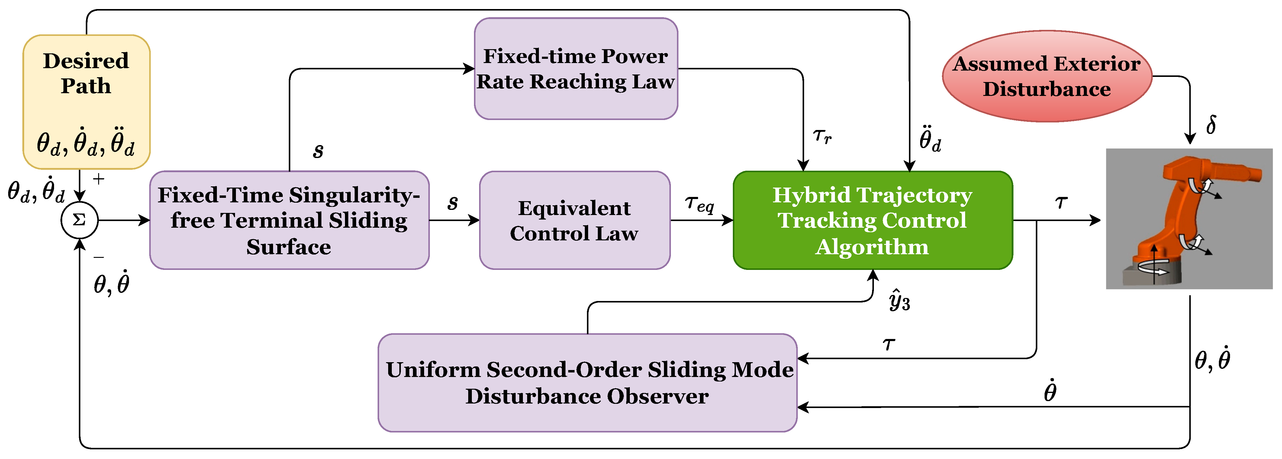
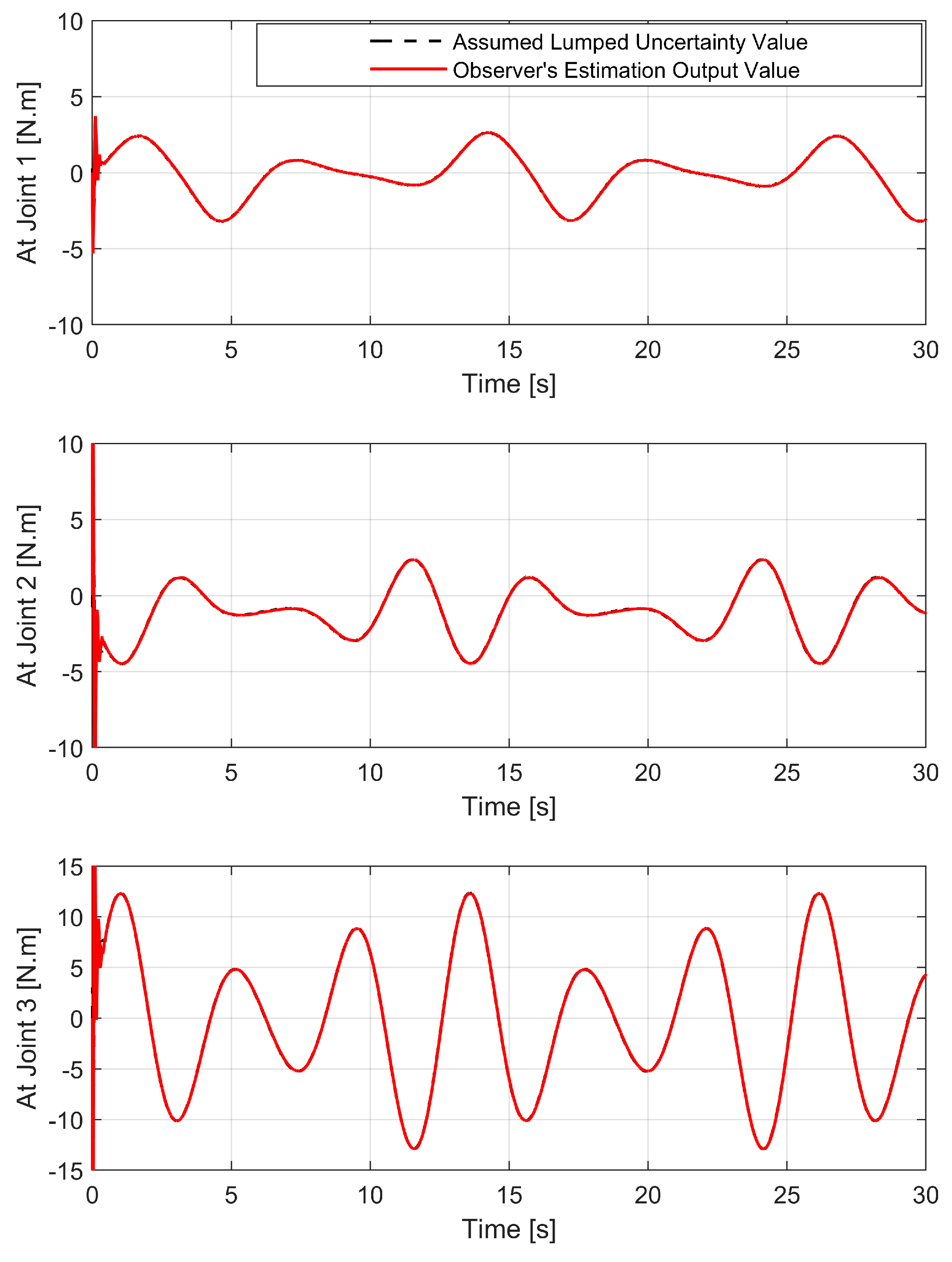
• The goal of attenuating the total uncertainties has been thoroughly solved with the proposal of USOSMDO. The observer not only accurately approximates the unknown components but also obtains them in fixed time.
• The FxSTSS is proposed to form a fixed-time convergence for the TCE to the sliding surface.
• For the design of the FxPRRL, we used a simple tuning function. In a bounded amount of time, the TCEs rapidly approaches the sliding surface thanks to this technique.
• The control proposal not only stabilizes with the global fixed-time convergence but also attains higher tracking accuracy compared to some state-of-the-art control systems such as SMC [39] and NFTSMC [40].
• The chattering problem is thoroughly addressed.
• Proof of the stability and settling time of the introduced techniques was sufficiently yielded.

The content of this paper is organized into five main sections. The first piece of content is the introduction. Section 2 is problem formulation. Section 3 provides the control. A discussion of simulated performance on a 3-DOF FARA-AT2 robot is presented in Section 4. Section 5 provides the conclusions from the obtained results of the study.

Some notions are provided for the reader’s convenience in our paper. $R^n$ is the real n-dimensional space; $R^{n \times m}$ is the set of m by n real matrices; ·^T is the transpose of; $\parallel ·\parallel$ is Euclidean norm of; $\left|·\right|$ is absolute value of; ${\lceil y\rfloor }^{\mu } = {\left|y\right|}^{\mu }\mathrm{sign}(y)$; $\frac{d}{dt}{\lceil y\rfloor }^{\mu } = \mu {\left|y\right|}^{\mu - 1}\stackrel{.}{y}$.

2. Problem Formulation

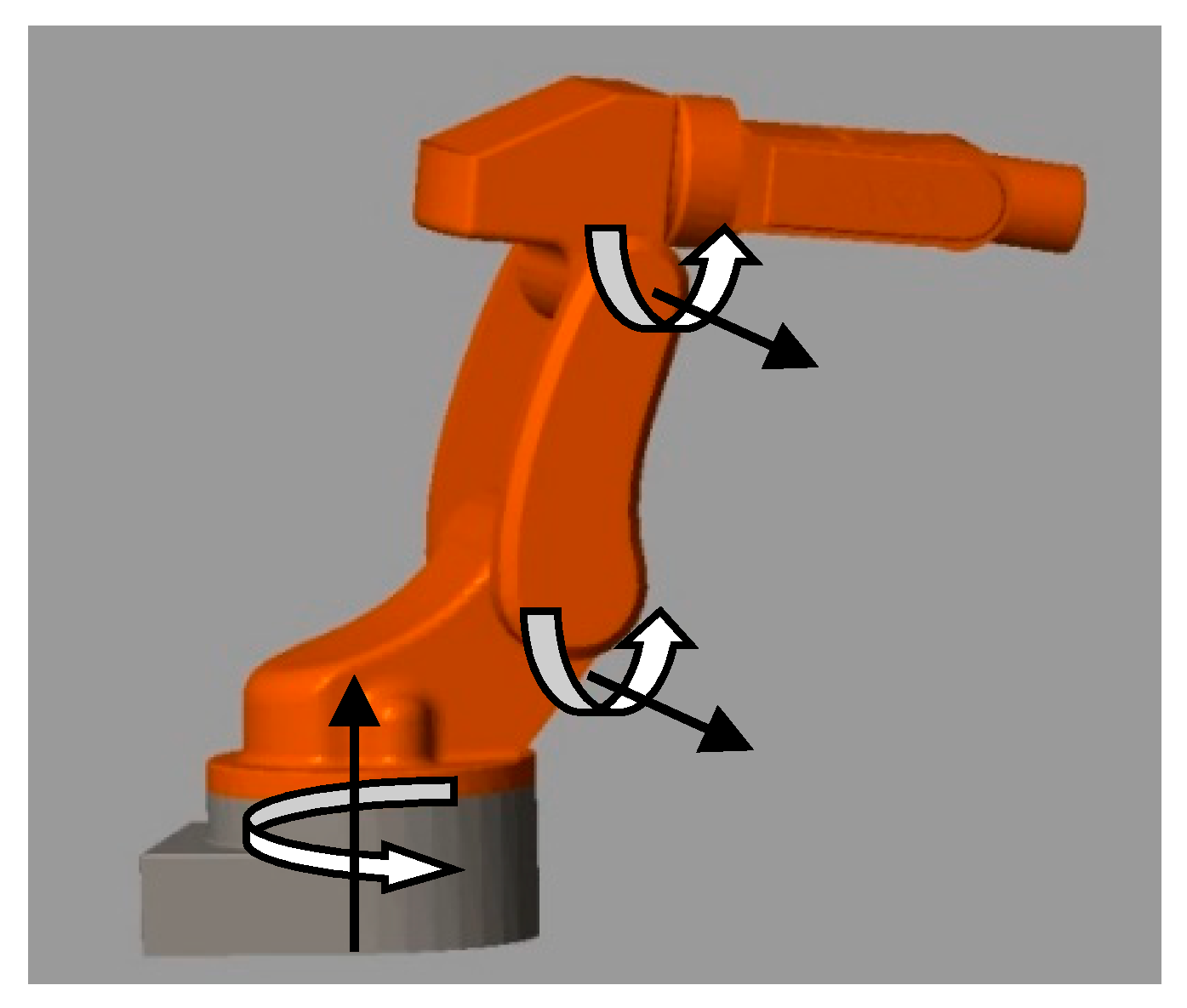
Description of Robot Manipulator Dynamics

The dynamics of an n-degree-of-freedom (DOF) robot manipulator are defined as [41]:

$$M(\theta )\stackrel{..}{\theta } + C(\theta ,\stackrel{.}{\theta })\stackrel{.}{\theta } + G(\theta ) + F_f(\stackrel{.}{\theta }) + \delta = \tau ,$$

(1)

where $\stackrel{..}{\theta },\stackrel{.}{\theta },\theta \in R^{n \times 1}$ are, respectively, acceleration vector, velocity vector, and position vector. $M(\theta )\in R^{n \times n}$, $C(\theta ,\stackrel{.}{\theta })\in R^{n \times n}$, and $G(\theta )\in R^{n \times 1}$ represent the inertia matrix, the centripetal-Coriolis matrix, and gravitation force vector, respectively. $F_f(\stackrel{.}{\theta })\in R^{n \times 1}$ is interior friction vector, $\delta$ represents exterior disturbance vector, and $\tau \in R^{n \times 1}$ is torque vector.

The existence of uncertainties in the RMs is inevitable. Therefore, Equation (1) is fully expressed in the below form:

$$(M_c(\theta ) + M_{\mathsf{\Delta }}(\theta ))\stackrel{..}{\theta } + (C_c(\theta ,\stackrel{.}{\theta }) + C_{\mathsf{\Delta }}(\theta ,\stackrel{.}{\theta }))\stackrel{.}{\theta } + (G_c(\theta ) + G_{\mathsf{\Delta }}(\theta )) + F_f(\stackrel{.}{\theta }) + \delta = \tau ,$$

(2)

where $M_{\mathsf{\Delta }}(\theta ),C_{\mathsf{\Delta }}(\theta ,\stackrel{.}{\theta }),G_{\mathsf{\Delta }}(\theta )$, and $F_f(\stackrel{.}{\theta })$ are unknown dynamics of the robot. $M_c(\theta )$, $C_c(\theta ,\stackrel{.}{\theta })$, and $G_c(\theta )$ are the calculated value of $M(\theta )$, $C(\theta ,\stackrel{.}{\theta })$, and $G(\theta )$. The lumped uncertainty can be considered a new variable. As a result, Equation (2) is transformed into:

$$M_c(\theta )\stackrel{..}{\theta } + C_c(\theta ,\stackrel{.}{\theta })\stackrel{.}{\theta } + G_c(\theta ) + \mathsf{\psi } = \tau ,$$

(3)

where $\mathsf{\psi } = M_{\mathsf{\Delta }}(\theta )\stackrel{..}{\theta } + C_{\mathsf{\Delta }}(\theta ,\stackrel{.}{\theta })\stackrel{.}{\theta } + G_{\mathsf{\Delta }}(\theta ) + F_f(\stackrel{.}{\theta }) + \delta$ is the lumped uncertainty.

For the purpose of tracking trajectories, these dynamic models must take into account nonmodular dynamics, coupled nonlinear dynamics, external disturbances, and parametric variations, all of which require robust control. Moreover, providing robots with superior control performance is not an easy matter. Therefore, the main purpose of the paper is to form a control system for RMs that not only stabilizes with the global fixed-time convergence but also attains better control performance compared to some state-of-the-art control systems, such as SMC and NFTSMC.

3. Control Design Preparation

3.1. Preliminaries

The following are some preliminaries regarding the finite-time stability/fixed-time stability and Lemmas.

Consider the following system

$$\dot{y} = f(y(t)),y(0) = y_0,f(0) = 0,y\in \mathrm{\Omega }\subset R^n,$$

(4)

where $f:\mathrm{\Omega } \times R^{+}\to R^n$ is a continuous function in an open neighborhood $\mathrm{\Omega }$ of the origin $y = 0$.

Definition 1 ([42]).

In Equation (4), the system’s origin is (locally) finite-time stable if it is Lyapunov stable and there is a convergence time function $T\left(y_0\right) > 0$ satisfying ${lim}_{t\to t_0 + T}y\left(t,y_0\right) = 0$ for any initial condition $y_0\in \mathrm{\Omega }$ at $t_0$.

Definition 2 ([42]).

The system (4) is termed the fixed-time stability if it is the finite-time stability and the convergence time function $T\left(y_0\right)$ is bounded by a positive number $T_{max}$, that is $T\left(y_0\right) \le T_{max}$.

Lemma 1 ([43,44]).

Consider the system, if there exist some constants $0 < {\rho }_0 < 1$ and ${\kappa }_0 > 0$ such that $\stackrel{.}{L}(y) \le -{\kappa }_0{L}^{{\rho }_0}(y)$, where $L(y)$ is the selected Lyapunov function, then the origin of the system (4) is a finite time stable.

Lemma 2 ([42]).

For a scalar system

$$\dot{y} = -{\psi }_0{\lceil y\rfloor }^{{\mu }_0} - {\kappa }_0{\lceil y\rfloor }^{{\rho }_0},$$

(5)

where ${\psi }_0 > 0,{\kappa }_0 > 0,{\mu }_0 > 1$ and $0 < {\rho }_0 < 1$. This system is fixed-time stable and its convergence time $T(y_0)$ is a bounded function by: $T(y_0) < T_{max}\triangleq \frac{1}{{\psi }_0({\mu }_0 - 1)} + \frac{1}{{\kappa }_0(1 - {\rho }_0)}$.

Lemma 3 ([34,45]).

For the system

$$\begin{array}{c}\hfill \left\{\begin{array}{c}{\dot{x}}_0 = -{\mathrm{\Pi }}_1{\mathrm{\Psi }}_{x_0} + x_1\hfill \\ {\dot{x}}_1 = -{\mathrm{\Pi }}_2{\mathrm{\Psi }}_{x_1} - \dot{d}\hfill \end{array}\right.,\end{array}$$

(6)

where ${\mathrm{\Psi }}_{x_0} = {\lceil x_0\rfloor }^{\frac{1}{2}} + A{\lceil x_0\rfloor }^{\frac{3}{2}}$ and ${\mathrm{\Psi }}_{x_1} = \frac{1}{2}{\lceil x_0\rfloor }^0 + 2A{x}_0 + \frac{3}{2}{A}^2{\lceil x_0\rfloor }^2$. If $A > 0$, $\left|\dot{d}\right| \le d_{max}$, $d_{max}$ is a positive constant, and ${\mathrm{\Pi }}_1$ and ${\mathrm{\Pi }}_2$ are obtained from the set:

$$\begin{array}{c}\hfill \mathrm{\Pi } = \left\{\left({\mathrm{\Pi }}_1,{\mathrm{\Pi }}_2\right)\in R^2\left|0 < {\mathrm{\Pi }}_1 \le 2\sqrt{d_{max}}\right.,{\mathrm{\Pi }}_2 > \frac{{\mathrm{\Pi }}_1^2}{4} + \frac{4d_{max}^2}{{\mathrm{\Pi }}_1^2}\right\}\cup \left\{\left({\mathrm{\Pi }}_1,{\mathrm{\Pi }}_2\right)\in R^2\left|{\mathrm{\Pi }}_1 > 2\sqrt{d_{max}}\right.,{\mathrm{\Pi }}_2 > 2d_{max}\right\}.\end{array}$$

Then, the states $x_0$ and $x_1$ will be converged to zero within a fixed time $T_0$ [45].

3.2. Design of an USOSMO

The objective of this subsection is to design a USOSMO that estimates all uncertain terms directly. A developed observer converges in finite time for bounded uncertain terms and for all initial conditions, with a uniformly bounded convergence time.

Transforming Equation (3) into the following form:

$$\stackrel{..}{\theta } = V(\theta )\tau + H(\theta ,\stackrel{.}{\theta }) + \varphi ,$$

(7)

where $H(\theta ,\stackrel{.}{\theta }) = -M_c^{-1}(\theta )(C_c(\theta ,\stackrel{.}{\theta })\stackrel{.}{\theta } + G_c(\theta )),V(\theta ) = M_c^{-1}(\theta )$, and $\varphi = -M_c^{-1}(\theta )\mathsf{\psi }$.

In the state space, Equation (7) becomes

$$\left\{\begin{array}{c}{\stackrel{.}{y}}_1 = y_2\hfill \\ {\stackrel{.}{y}}_2 = V(y_1)\tau + H(y_1,y_2) + y_3\hfill \end{array}\right.,$$

(8)

where $y_1 = \theta \in R^n$, $y_2 = \stackrel{.}{\theta }\in R^n$, and $y_3 = \varphi$.

For the system (8), the USOSMO is designed to achieve precisely the estimation of the lumped uncertainty:

$$\begin{array}{c}\hfill \left\{\begin{array}{c}{\tilde{y}}_2 = y_2 - {\widehat{y}}_2\\ {\dot{\widehat{y}}}_2 = V(y_1)\tau + H(y_1,y_2) + {\widehat{y}}_3 + {\xi }_1{\mathrm{\Psi }}_1\left({\tilde{y}}_2\right)\\ {\dot{\widehat{y}}}_3 = -{\xi }_2{\mathrm{\Psi }}_2\left({\tilde{y}}_2\right)\end{array}\right.,\end{array}$$

(9)

where ${\mathrm{\Psi }}_1\left({\tilde{y}}_2\right) = {\left[{\tilde{y}}_2\right]}^{\frac{1}{2}} + \gamma {\left[{\tilde{y}}_2\right]}^{\frac{3}{2}}$ and ${\mathrm{\Psi }}_2\left({\tilde{y}}_2\right) = \frac{1}{2}{\left[{\tilde{y}}_2\right]}^0 + 2\gamma {\tilde{y}}_2 + \frac{3}{2}{\gamma }^2{\left[{\tilde{y}}_2\right]}^2$. $y_2$ has an approximate value of ${\widehat{y}}_2$. ${\xi }_1$, ${\xi }_2$, and $\gamma$ represent the observer’s parameters. ${\xi }_1$ and ${\xi }_2$ are selected based on Lemma 3.

The synthesis of the USOSMO is described by the below theorem.

Theorem 1.

For the robot system described as Equation (8), if the condition $|{\stackrel{.}{y}}_3| \le d_{max}$ is satisfied, $d_{max}$ is a positive constant, then the estimated value ${\widehat{y}}_3$ from USOSMO output (9) will attain the true value $y_3$ in fixed time.

Proof of Theorem 1.

The USOSMO’s output errors are determined by

$$\begin{array}{c}\hfill \left\{\begin{array}{c}{\tilde{y}}_2 = y_2 - {\widehat{y}}_2\hfill \\ {\tilde{y}}_3 = {\widehat{y}}_3 - y_3\hfill \end{array}\right..\end{array}$$

(10)

By utilizing Equation (9), we can find the derivative of Equation (10) based on time, as follows:

$$\begin{array}{c}\hfill \left\{\begin{array}{c}{\dot{\tilde{y}}}_2 = -{\xi }_1{\mathrm{\Psi }}_1\left({\tilde{y}}_2\right) + {\tilde{y}}_3\hfill \\ {\dot{\tilde{y}}}_3 = -{\xi }_2{\mathrm{\Psi }}_2\left({\tilde{y}}_2\right) - {\dot{y}}_3\hfill \end{array}\right.,\end{array}$$

(11)

where ${\tilde{y}}_3$ is the USOSMO’s estimation error.

Take a look at Equation (11), it is a uniformly exact convergent according to Lemma 3. That means ${\tilde{y}}_2 = 0$ and ${\tilde{y}}_3 = 0$ in fixed time $T_0$ as Lemma 3.

This proof is completed. □

3.3. Design of FxSTSS

Define, respectively, the position and velocity control errors as $y_{1e} = y_1 - y_{1d}$ and $y_{2e} = y_2 - {\stackrel{.}{y}}_{1d}$. $y_e = {\left[\begin{array}{cc}{y}_{1e}& y_{2e}\end{array}\right]}^T$ is vector of the TCE. Therefore, Equation (8) is reconstructed as

$$\left\{\begin{array}{c}{\stackrel{.}{y}}_{1e} = y_{2e}\hfill \\ {\stackrel{.}{y}}_{2e} = V(y_1)\tau + H(y_1,y_2) + y_3 - {\stackrel{..}{y}}_{1d}\hfill \end{array}\right..$$

(12)

To obtain singularity-free and provide fixed time convergence, the novel FxSTSS is proposed as follows:

$$s = y_{1e} + \frac{1}{{\kappa }_1^{\frac{1}{{\rho }_1}}}{\left[{\psi }_1{\lceil y_{1e}\rfloor }^{{\mu }_1} + {\stackrel{.}{y}}_{1e}\right]}^{\frac{1}{{\rho }_1}},$$

(13)

where ${\psi }_1 > 0,{\kappa }_1 > 0,{\mu }_1 > 1$, and $\frac{1}{2} < {\rho }_1 < 1$.

In the control system design subsection, we will examine the singularity problem formed from the sliding surface with a detailed analysis.

When the FxSTSS (13) converges to zero, $s = 0$, we can obtain

$${\stackrel{.}{y}}_{1e} = -{\psi }_1{\lceil y_{1e}\rfloor }^{{\mu }_1} - {\kappa }_1{\lceil y_{1e}\rfloor }^{{\rho }_1}.$$

(14)

In the same way that Lemma 2 stated, the FxSTSS (13) possesses the same characteristics as the sliding surface in Ref. [42]. Therefore, it achieves a fixed-time convergence with the settling time $T(y_{e_0}) < T_{max}\triangleq \frac{1}{{\psi }_1({\mu }_1 - 1)} + \frac{1}{{\kappa }_1(1 - {\rho }_1)}$, $y_{e_0} = y_e(0)$.

3.4. Design of the Proposed HTCA

Set $\mathrm{Y} = {\psi }_1{\lceil y_{1e}\rfloor }^{{\mu }_1} + {\stackrel{.}{y}}_{1e}$, so, ${\left|\mathrm{Y}\right|}^{\frac{1}{{\rho }_1} - 1} = {\left[{\psi }_1{\lceil y_{1e}\rfloor }^{{\mu }_1} + {\stackrel{.}{y}}_{1e}\right]}^{\frac{1}{{\rho }_1} - 1}$. Then, differentiating the FxSTSS (13) according to time, we obtain

$$\stackrel{.}{s} = {\stackrel{.}{y}}_{1e} + \frac{1}{{\kappa }_1^{\frac{1}{{\rho }_1}}}\frac{1}{{\rho }_1}{\left|\mathrm{Y}\right|}^{\frac{1}{{\rho }_1} - 1}\left({\psi }_1{\mu }_1{\lceil y_{1e}\rfloor }^{{\mu }_1 - 1}{\stackrel{.}{y}}_{1e} + {\stackrel{..}{y}}_{1e}\right).$$

(15)

Inserting (12) into (15) yields

$$\stackrel{.}{s} = {\stackrel{.}{y}}_{1e} + \frac{1}{{\kappa }_1^{\frac{1}{{\rho }_1}}}\frac{1}{{\rho }_1}{\left|\mathrm{Y}\right|}^{\frac{1}{{\rho }_1} - 1}\left({\psi }_1{\mu }_1{\lceil y_{1e}\rfloor }^{{\mu }_1 - 1}{\stackrel{.}{y}}_{1e} + V(y_1)\tau + H(y_1,y_2) + y_3 - {\stackrel{..}{y}}_{1d}\right).$$

(16)

Based on Equation (16), an overview of the proposed HTCA is synthesized below

$$\tau = {\tau }_{eq} + {\tau }_{ob} + {\tau }_r,$$

(17)

where

$${\tau }_{eq} = -V^{+}\left({\psi }_1{\mu }_1{\lceil y_{1e}\rfloor }^{{\mu }_1 - 1}{\stackrel{.}{y}}_{1e} + H(y_1,y_2) - {\stackrel{..}{y}}_{1d}\right) - V^{+}{\kappa }_1^{\frac{1}{{\rho }_1}}{\rho }_1{\left|\mathrm{Y}\right|}^{1 - \frac{1}{{\rho }_1}}{\stackrel{.}{y}}_{1e},$$

${\tau }_{ob}$ is provided by Observer (9)

$${\tau }_{ob} = -V^{+}{\widehat{y}}_3,$$

and ${\tau }_r$ is the FxPRRL

$${\tau }_r = -V^{+}{\kappa }_2\left(1 + {\psi }_2^2{\left|s\right|}^{2(1 - {\rho }_2)}\right){\left|s\right|}^{{\rho }_2}\mathrm{sign}(s).$$

$V^{+}$ is the pseudo inverse of the V. ${\kappa }_2,{\psi }_2 > 0$, and $0 < {\rho }_2 < 1$ are constants.

Remark 1.

With the sliding surface designed in Equation (13), the ${\tau }_{eq}$ exists the term ${\left|\mathrm{Y}\right|}^{1 - \frac{1}{{\rho }_1}}{\stackrel{.}{y}}_{1e}$. Interestingly, this term does not produce a singularity. When ${\stackrel{.}{y}}_{1e} \ne 0,y_{1e} = 0$, we have $|{\stackrel{.}{y}}_{1e}{|}^{1 - \frac{1}{{\rho }_1}}{\stackrel{.}{y}}_{1e} \ge {\stackrel{.}{y}}_{1e}^{2 - \frac{1}{{\rho }_1}},2 - \frac{1}{{\rho }_1}$ is a positive power term.

Theorem 2.

Using the estimated disturbance ${\widehat{y}}_3$ from the observer (9), the FxSTSS (13), and the FxPRRL ${\tau }_r$, the controller (17) will provide convergence and stability for the robot system (8) within a fixed time.

Remark 2.

The stabilization process of this method is summarized into three phases as follows: firstly, the estimated value of disturbance ${\widehat{y}}_3$ from USOSMO output (9) will attain the true value of disturbance $y_3$ in fixed time, that means ${\widehat{y}}_3 = y_3$, i.e., ${\tilde{y}}_3 = 0$; secondly, the TCEs will be converged to the FxSTSS with the bounded reaching time as $T_r < T_{max}\triangleq \frac{\pi }{2{\kappa }_2{\psi }_2(1 - {\rho }_2)}$; finally, the TCEs maintain along the FxSTSS to equilibrium with settling time $T(y_{e_0}) < T_{max}\triangleq \frac{1}{{\psi }_1({\mu }_1 - 1)} + \frac{1}{{\kappa }_1(1 - {\rho }_1)}$.

Proof of Theorem 2.

Adding (17) to (16) obtains

$$\stackrel{.}{s} = -{\kappa }_2\left(1 + {\psi }_2^2{\left|s\right|}^{2(1 - {\rho }_2)}\right){\left|s\right|}^{{\rho }_2}\mathrm{sign}(s) - {\tilde{y}}_3.$$

(18)

After the first phase, ${\tilde{y}}_3 = 0$, so, $\stackrel{.}{s} = -{\kappa }_2\left(1 + {\psi }_2^2{\left|s\right|}^{2(1 - {\rho }_2)}\right){\left|s\right|}^{{\rho }_2}\mathrm{sign}(s)$.

Choosing a candidate Lyapunov function as $L = \frac{1}{2}{s}^2$ then, differentiating it, one obtains

$$\begin{array}{c}\stackrel{.}{L} = -s\left({\kappa }_2\left(1 + {\psi }_2^2|s{|}^{2(1 - {\rho }_2)}\right)|s{|}^{{\rho }_2}\mathrm{sign}(s)\right)\hfill \\ = -{\kappa }_2\left(1 + {\psi }_2^2|s{|}^{2(1 - {\rho }_2)}\right)|s{|}^{{\rho }_2 + 1}\hfill \\ \le -{\kappa }_2\left(1 + {\psi }_2^2|s{|}^{2(1 - {\rho }_2)}\right)|s{|}^{{\rho }_2 + 1}\hfill \\ \le -{\kappa }_2|s{|}^{{\rho }_2 + 1} = -\sqrt{2}{\kappa }_2{(L)}^{\frac{{\rho }_2 + 1}{2}}\hfill \end{array}.$$

(19)

Note that $0 < {\rho }_2 < 1$; then, we have $0 < \frac{{\rho }_2 + 1}{2} < 1$. Thus, the origin s is globally finite-time stable according to Lemma 1. The reaching time can be computed by solving differential Equation (18) with ${\tilde{y}}_3 = 0$:

$$\stackrel{.}{s} = -{\kappa }_2\left(1 + {\psi }_2^2{\left|s\right|}^{2(1 - {\rho }_2)}\right){\left|s\right|}^{{\rho }_2}\mathrm{sign}(s).$$

(20)

Rewriting Equation (20) as

$$\frac{{\psi }_2(1 - {\rho }_2){\left|s\right|}^{-{\rho }_2}}{1 + {\psi }_2^2{\left|s\right|}^{2(1 - {\rho }_2)}}\mathrm{sign}(s)ds = -{\kappa }_2{\psi }_2(1 - {\rho }_2)dt.$$

(21)

Defining $T_r = T(s_0)$ to be the settling time that is gained by solving Equation (20).

Integrating Equation (21) from the time 0 to $T_r$ gives

$$\underset{s(0)}{\overset{s(T_r)}{\int }}\frac{{\psi }_2(1 - {\rho }_2)|s{|}^{-{\rho }_2}}{1 + {\psi }_2^2|s{|}^{2(1 - {\rho }_2)}}\mathrm{sign}(s)ds = \underset{0}{\overset{T_r}{\int }}-{\kappa }_2{\psi }_2(1 - {\rho }_2)dt.$$

(22)

If $s > 0$ for $0 \le t \le T_r$, then

$${\left.arctan\left({\psi }_2{s}^{1 - {\rho }_2}\right)\right|}_{s(0)}^{s(T_r)} = {\left.-{\kappa }_2{\psi }_2(1 - {\rho }_2)t\right|}_0^{T_r}.$$

(23)

We have $s(T_r) = 0$, so

$$-arctan\left({\psi }_2{s}_0^{1 - {\rho }_2}\right) = -{\kappa }_2{\psi }_2(1 - {\rho }_2)T_r.$$

(24)

Consequently, $T_r$ can be given as

$$T_r = \frac{arctan\left({\psi }_2{s}_0^{1 - {\rho }_2}\right)}{{\kappa }_2{\psi }_2(1 - {\rho }_2)}.$$

(25)

If $s < 0$ for $0 \le t \le T_r$, then $T_r$ can be obtained with the same way of calculation

$$T_r = \frac{arctan\left({\psi }_2{(-s_0)}^{1 - {\rho }_2}\right)}{{\kappa }_2{\psi }_2(1 - {\rho }_2)}.$$

(26)

Therefore, the settling time is

$$T_r = \frac{arctan\left({\psi }_2{\left|s_0\right|}^{1 - {\rho }_2}\right)}{{\kappa }_2{\psi }_2(1 - {\rho }_2)} < T_{max}\triangleq \frac{\pi }{2{\kappa }_2{\psi }_2(1 - {\rho }_2)}.$$

(27)

The proof has been fully confirmed. □

Figure 1 shows the proposed control structure.

4. Simulations

This section shows and discusses the simulation performance from three different methods, including the suggested synthesis, the conventional SMC, and NFTSMC on the designed 3-DOF FARA-AT2 robot. SOLIDWORKS is used to build the mechanical model of this robot. A geometric graphic model of the FARA-AT2 robot is depicted in Figure 2. The geometry parameters are taken from the Samsung FARA-AT2 robot, as shown in Figure 3. We then use the Simmechanics toolbox to export a robot manipulator model to MATLAB/SIMULINK environment. The dynamical computations of 3-DOF FARA-AT2 robot are based on Refs. [41,46]. The Euler method was used to find the solutions of differential equations with an ODE5 $0.001$ s time step in MATLAB/SIMULINK.

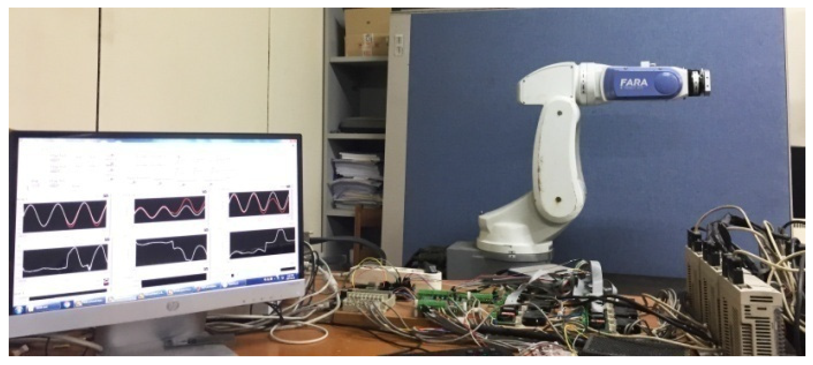
4.1. System Configuration and Parameter Selection for the Robot

Table 1. Essential parameters for the design of a FARA-AT2 robot.

Description	Link 1	Link 2	Link 3
Length (m)	$l_1 = 0.15$	$l_2 = 0.255$	$l_3 = 0.41$
Weight (kg)	$m_1 = 56.5$	$m_2 = 35.6$	$m_3 = 58.9$
Center of Mass (mm)	$\begin{array}{c}{l}_{c1x} = -98.3 \times {10}^{-3}\\ l_{c1y} = -2.9 \times {10}^{-3}\\ l_{c1z} = -85.4 \times {10}^{-3}\end{array}$	$\begin{array}{c}{l}_{c2x} = -5.5 \times {10}^{-3}\\ l_{c2y} = 0.001 \times {10}^{-3}\\ l_{c2z} = -156.9 \times {10}^{-3}\end{array}$	$\begin{array}{c}{l}_{c3x} = 54.6 \times {10}^{-3}\\ l_{c3y} = -0.01 \times {10}^{-3}\\ l_{c3z} = 80.5 \times {10}^{-3}\end{array}$
Inertia (kg·m2)	$\begin{array}{c}\hfill I_{1xx} = 0.39\hfill \\ \hfill I_{1yy} = 0.59\hfill \\ \hfill I_{1zz} = 0.56\hfill \end{array}$	$\begin{array}{c}\hfill I_{2xx} = 0.76\hfill \\ \hfill I_{2yy} = 0.44\hfill \\ \hfill I_{2zz} = 0.39\hfill \end{array}$	$\begin{array}{c}\hfill I_{3xx} = 0.22\hfill \\ \hfill I_{3yy} = 1.2\hfill \\ \hfill I_{3zz} = 1.2\hfill \end{array}$

contains the parameters required for the design of the robot and its dynamic calculation.

In joint space, the robot is required to track the trajectory below accurately:

$$\left\{\begin{array}{c}{\theta }_{1d} = 0.5cos(t/2) - 0.5\hfill \\ {\theta }_{2d} = 0.3cos(t) - 0.3\hfill \\ {\theta }_{3d} = 0.2cos(t) - 0.2\hfill \end{array}\right.\left[\mathrm{rad}\right].$$

(28)

To evaluate the estimation ability of the observer, the efficiency, and the robustness of the proposed controller, we assume that there are effects of uncertain factors on the robot, such as external disturbances and interior frictions. Each joint has assumed interior friction of $F_{f1}(\stackrel{.}{\theta }) = 0.1\mathrm{sign}({\stackrel{.}{\theta }}_1) + 2{\stackrel{.}{\theta }}_1[\mathrm{N}·\mathrm{m}]$, $F_{f2}(\stackrel{.}{\theta }) = 0.1\mathrm{sign}({\stackrel{.}{\theta }}_2) + 2{\stackrel{.}{\theta }}_2[\mathrm{N}·\mathrm{m}]$, and $F_{f3}(\stackrel{.}{\theta }) = 0.1\mathrm{sign}({\stackrel{.}{\theta }}_3) + 2{\stackrel{.}{\theta }}_3[\mathrm{N}·\mathrm{m}]$, respectively. Each joint has assumed exterior disturbance of ${\delta }_1 = 4sin(t)[\mathrm{N}·\mathrm{m}]$, ${\delta }_2 = 5sin(t)[\mathrm{N}·\mathrm{m}]$, and ${\delta }_3 = 6sin(t)[\mathrm{N}·\mathrm{m}]$.

The proposed controller is compared to a newly published NFTSMC [40] and the conventional SMC [39] for controlling robots about its control performance. Since the structure of each controller is different, ensuring a fair comparison is not easy. Therefore, to ensure a comparison that is as fair as possible, we used the control parameters of NFTSMC from Ref. [40] for simulation on the robot. The control parameters of the proposed controller are selected experimentally to achieve good performance and bring out its full possibility. The robot states are considered with the same initial conditions.

Table 2. Parameters of the proposed controller.

Description	Symbol	Value
USOSMO (9)	${\xi }_1,{\xi }_2,\gamma$	$3,40,2\sqrt{20}$
FxSTSS (13)	${\psi }_1,{\kappa }_1,{\mu }_1,{\rho }_1$	$0.2,3,1.4,0.6$
FxPRRL(17)	${\psi }_2,{\kappa }_2,{\rho }_2$	$10,40,0.6$

provides the control parameters selected for the proposed method.

The conventional SMC’s [39] control input is

$$\left\{\begin{array}{c}s = {\stackrel{.}{y}}_{1e} + {\psi }_3{y}_{1e}\hfill \\ \tau = V^{-1}(y_1)({\tau }_{eq} + {\tau }_r)\hfill \\ {\tau }_{eq} = {\stackrel{..}{y}}_{1d} - H(y_1,y_2) - {\psi }_3{\stackrel{.}{y}}_{1e}\hfill \\ {\tau }_r = -({\kappa }_{3}s + {\kappa }_4\mathrm{sign}(s))\hfill \end{array}\right.,$$

(29)

in which ${\psi }_3,{\kappa }_3$, and ${\kappa }_4$ are positive constants.

The NFTSMC [40] was designed with the following control law

$$\left\{\begin{array}{c}s = y_{1e} + {\psi }_4{(1 + y_{1e}^2)}^{\frac{q}{p}}arctan(y_{1e}){\stackrel{.}{y}}_{1e}^{\frac{q}{p}}\hfill \\ \tau = V^{-1}(y_1)({\tau }_{eq} + {\tau }_r)\hfill \\ {\tau }_{eq} = {\stackrel{..}{y}}_{1d} - H(y_1,y_2) + \frac{p}{{\psi }_{4}q}{(1 + y_{1e}^2)}^{\frac{q}{p} - 1}(1 + \frac{2q}{p}{y}_{1e}arctan(y_{1e}){\stackrel{.}{y}}_{1e}^{2 - \frac{q}{p}})\hfill \\ {\tau }_r = -({\kappa }_{5}s + {\kappa }_6\mathrm{sign}(s))\hfill \end{array}\right.,$$

(30)

in which $q,p$ are positive odd integers, $1 < \frac{q}{p} < 2$, ${\psi }_4,{\kappa }_5$, and ${\kappa }_6$ are positive constants.

The accuracy of the TCEs is calculated by using the roots–mean–square algorithm (RMSA) as Equation (31) when the TCEs are in the sliding motion phase to equilibrium. Therefore, the TCEs are calculated in the period of time between the 2nd and 30th seconds in the simulation. The computed results are shown in

Table 3. RMSEs via three control algorithms.

Control System	${\mathit{E}}_1$	${\mathit{E}}_2$	${\mathit{E}}_3$
SMC	$\begin{array}{c}6 \times {10}^{-4}\hfill \end{array}$	$\begin{array}{c}1.8 \times {10}^{-3}\hfill \end{array}$	$\begin{array}{c}4.5 \times {10}^{-3}\hfill \end{array}$
NFTSMC	$\begin{array}{c}2.34 \times {10}^{-5}\hfill \end{array}$	$\begin{array}{c}1.473 \times {10}^{-4}\hfill \end{array}$	$\begin{array}{c}7.561 \times {10}^{-4}\hfill \end{array}$
Proposed Synthesis	$\begin{array}{c}2.74 \times {10}^{-6}\hfill \end{array}$	$\begin{array}{c}7.78 \times {10}^{-6}\hfill \end{array}$	$\begin{array}{c}1.991 \times {10}^{-5}\hfill \end{array}$

.

$$\begin{array}{c}{E}_1 = \sqrt{\frac{1}{\mathrm{K}}{\displaystyle \sum _{i = 1}^{\mathrm{K}}}{\left|\left({\theta }_{d1i} - {\theta }_{1i}\right)\right|}^2};E_2 = \sqrt{\frac{1}{\mathrm{K}}{\displaystyle \sum _{i = 1}^{\mathrm{K}}}{\left|\left({\theta }_{d2i} - {\theta }_{2i}\right)\right|}^2};E_3 = \sqrt{\frac{1}{\mathrm{K}}{\displaystyle \sum _{i = 1}^{\mathrm{K}}}{\left|\left({\theta }_{d3i} - {\theta }_{3i}\right)\right|}^2},\hfill \end{array}$$

(31)

in which $\mathrm{K}$ is the number of the calculated samples. Roots–mean–square error (RMSE) of Joint 1, Joint 2, and Joint 3 are $E_1$, $E_2$, and $E_3$, respectively. ${[{\theta }_{1i},{\theta }_{2i},{\theta }_{3i}]}^T$ is the real joint angle vector and ${[{\theta }_{d1i},{\theta }_{d2i},{\theta }_{d3i}]}^T$ is the desired joint angle vector at time index i.

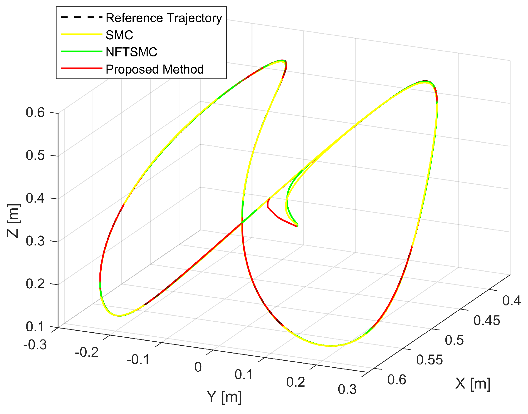
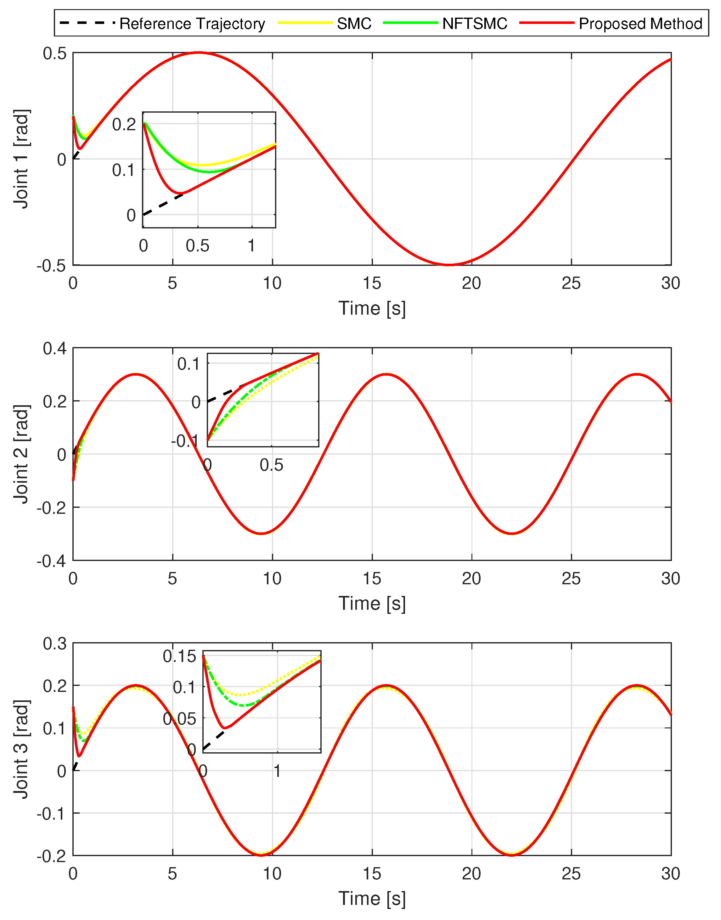
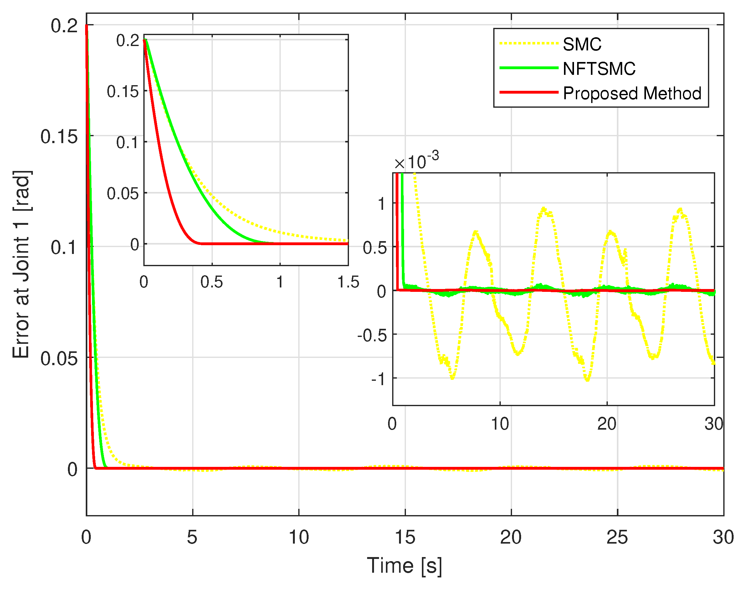
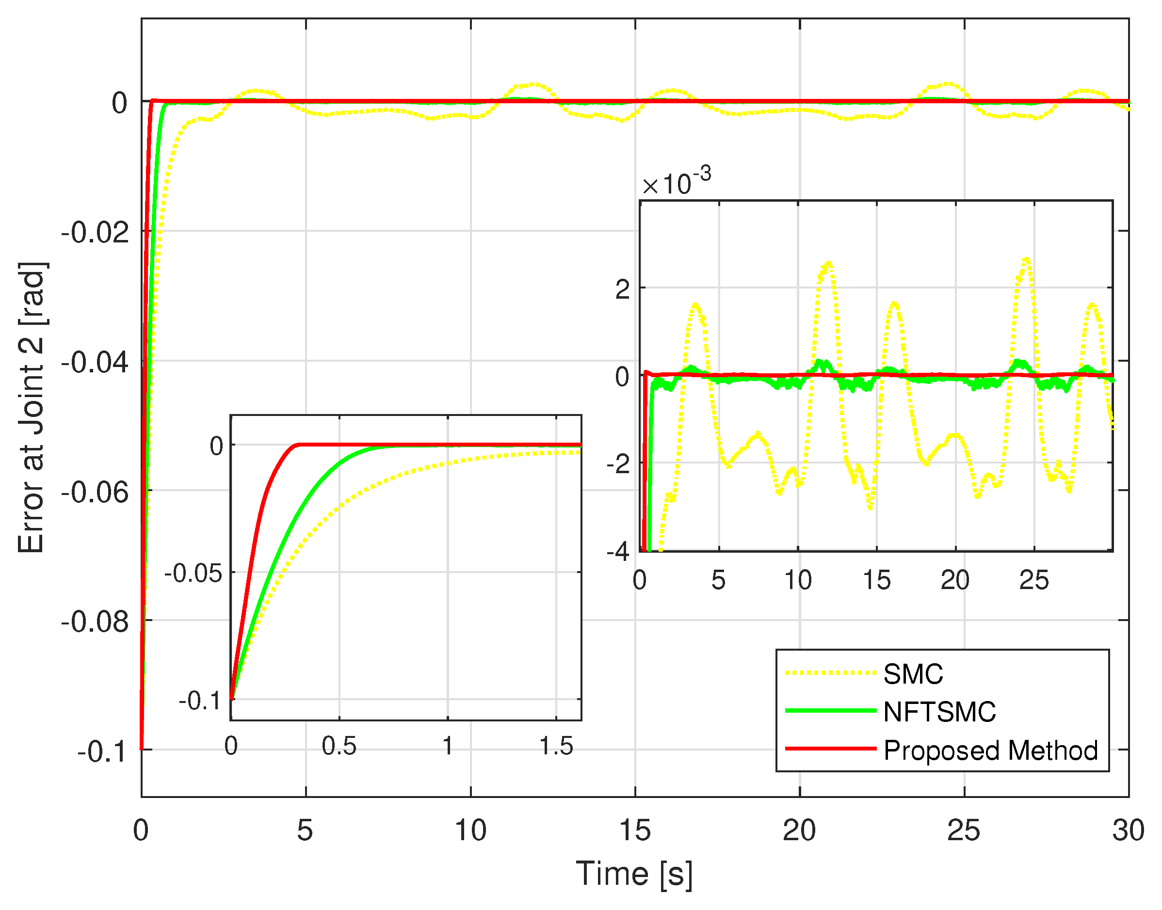
4.2. Discussion of Performance Results

Firstly, the approximation ability of the proposed USOSMO is discussed. The estimation performance from observer is shown in Figure 4. As shown in Figure 4, the proposed USOSMO achieved fast convergence and high accuracy of disturbance estimation. The estimated value ${\widehat{y}}_3$ from the USOSMO output (9) quickly attained the true value $y_3$ in fixed time. USOSMO’s estimation errors have a fixed-time uniform convergence regardless of the initial condition. This is really important for the robustness improvement of the controller and obtaining the smallest possible TCEs. After that, we will analyze any tracking issues from the simulation results.

Figure 5 shows the real trajectory of the robot’s end-effector compared to the desired trajectory. Figure 6 depicts the real trajectory positions of the robot joint generated by three different methods compared to the desired path. Each method can be successfully used to control the robot to track its desired path. Figure 7, Figure 8 and Figure 9 show, respectively, the TCEs at each joint between the real trajectory position and the desired path. Looking at Figure 7, Figure 8 and Figure 9 and comparing the results in Table 3, the suggested control synthesis proves its superiority in trajectory tracking problems when minimizing the smallest TCEs among the three controllers. The NFTSMC [40] is a recent modern control method, so it also achieved relatively high tracking accuracy, its accuracy is higher than the conventional SMC.

In convergence terms, the suggested HTCA also has the best performance, its TCEs quickly reach equilibrium in the shortest time, while the TCEs of the NFTSMC converge to equilibrium faster than those of the conventional SMC.

In the control torque signal of the proposed method, the chattering behavior has been minimized to the smallest possible extent, as shown in Figure 10, because its discontinuous control law has been removed. Although a discontinuous control law is not used to deal with uncertain components, the robustness of the controller is achieved at a high level so that it provides good tracking accuracy. Due to using the same sliding gain to cope with the effects of uncertainties, the other two methods have similar chattering behavior. It can be concluded that the combination of the proposed USOSMO and the proposed FxPRRL is a very good solution to deal with the influence of uncertainty and chattering.

5. Conclusions

As part of our recent research, we investigated the HTCA for robot manipulators with uncertain dynamics and the impact of external disturbances. The USOSMDO was proposed to estimate directly the lumped uncertainties, thereby achieving the active disturbance rejection. Then, by integrating the TSMC and the developed USOSMDO, our control synthesis was formed, and not only the fixed-time convergence of the TCEs but also the high tracking accuracy was guaranteed. In addition, the chattering problem also was handled almost thoroughly. Finally, numerical simulations verified the benefits and effectiveness of the HTCA to a designed 3-DOF FARA-AT2 robot.

In future work, we will apply the developed method to the real FARA-AT2 robot that is available in our laboratory as depicted in Figure 3.

References

1. Codourey, A. Dynamic modeling of parallel robots for computed-torque control implementation. Int. J. Robot. Res. 1998, 17, 1325–1336. [Google Scholar] [CrossRef]
2. Hernández-Guzmán, V.; Orrante-Sakanassi, J. Global PID control of robot manipulators equipped with PMSMs. Asian J. Control 2018, 20, 236–249. [Google Scholar] [CrossRef]
3. Adhikary, N.; Mahanta, C. Sliding mode control of position commanded robot manipulators. Control Eng. Pract. 2018, 81, 183–198. [Google Scholar] [CrossRef]
4. Islam, S.; Liu, X.P. Robust sliding mode control for robot manipulators. IEEE Trans. Ind. Electron. 2010, 58, 2444–2453. [Google Scholar] [CrossRef]
5. Slotine, J.J.E.; Li, W. Composite adaptive control of robot manipulators. Automatica 1989, 25, 509–519. [Google Scholar] [CrossRef]
6. Sadati, N.; Ghadami, R. Adaptive multi-model sliding mode control of robotic manipulators using soft computing. Neurocomputing 2008, 71, 2702–2710. [Google Scholar] [CrossRef]
7. Tran, X.T.; Kang, H.J. Adaptive hybrid high-order terminal sliding mode control of MIMO uncertain nonlinear systems and its application to robot manipulators. Int. J. Precis. Eng. Manuf. 2015, 16, 255–266. [Google Scholar] [CrossRef]
8. Le, T.D.; Kang, H.J.; Suh, Y.S. Chattering-free neuro-sliding mode control of 2-DOF planar parallel manipulators. Int. J. Adv. Robot. Syst. 2013, 10, 22. [Google Scholar] [CrossRef]
9. Wai, R.J. Fuzzy sliding-mode control using adaptive tuning technique. IEEE Trans. Ind. Electron. 2007, 54, 586–594. [Google Scholar] [CrossRef]
10. Gao, W.; Hung, J.C. Variable structure control of nonlinear systems: A new approach. IEEE Trans. Ind. Electron. 1993, 40, 45–55. [Google Scholar]
11. Pan, H.; Zhang, G.; Ouyang, H.; Mei, L. A Novel Global Fast Terminal Sliding Mode Control Scheme For Second-Order Systems. IEEE Access 2020, 8, 22758–22769. [Google Scholar] [CrossRef]
12. Hu, H.X.; Wen, G.; Yu, W.; Cao, J.; Huang, T. Finite-time coordination behavior of multiple Euler–Lagrange systems in cooperation-competition networks. IEEE Trans. Cybern. 2019, 49, 2967–2979. [Google Scholar] [CrossRef]
13. Hong, Y.; Xu, Y.; Huang, J. Finite-time control for robot manipulators. Syst. Control Lett. 2002, 46, 243–253. [Google Scholar] [CrossRef]
14. Bhat, S.P.; Bernstein, D.S. Geometric homogeneity with applications to finite-time stability. Math. Control. Signals Syst. 2005, 17, 101–127. [Google Scholar] [CrossRef] [Green Version]
15. Van, M.; Ge, S.S.; Ren, H. Finite time fault tolerant control for robot manipulators using time delay estimation and continuous nonsingular fast terminal sliding mode control. IEEE Trans. Cybern. 2017, 47, 1681–1693. [Google Scholar] [CrossRef]
16. Tran, X.T.; Kang, H.J. Robust adaptive chatter-free finite-time control method for chaos control and (anti-) synchronization of uncertain (hyper) chaotic systems. Nonlinear Dyn. 2015, 80, 637–651. [Google Scholar] [CrossRef]
17. Galicki, M. Finite-time control of robotic manipulators. Automatica 2015, 51, 49–54. [Google Scholar] [CrossRef]
18. Truong, T.N.; Vo, A.T.; Kang, H.J. A backstepping global fast terminal sliding mode control for trajectory tracking control of industrial robotic manipulators. IEEE Access 2021, 9, 31921–31931. [Google Scholar] [CrossRef]
19. Truong, T.N.; Vo, A.T.; Kang, H.J.; Van, M. A Novel Active Fault-Tolerant Tracking Control for Robot Manipulators with Finite-Time Stability. Sensors 2021, 21, 8101. [Google Scholar] [CrossRef]
20. Nguyen, V.C.; Vo, A.T.; Kang, H.J. A finite-time fault-tolerant control using non-singular fast terminal sliding mode control and third-order sliding mode observer for robotic manipulators. IEEE Access 2021, 9, 31225–31235. [Google Scholar] [CrossRef]
21. Li, R.; Yang, L.; Chen, Y.; Lai, G. Adaptive Sliding Mode Control of Robot Manipulators with System Failures. Mathematics 2022, 10, 339. [Google Scholar] [CrossRef]
22. Tran, X.T.; Kang, H.J. TS fuzzy model-based robust finite time control for uncertain nonlinear systems. Proc. Inst. Mech. Eng. Part C J. Mech. Eng. Sci. 2015, 229, 2174–2186. [Google Scholar] [CrossRef]
23. Vo, A.T.; Kang, H.J. An Adaptive Neural Non-Singular Fast-Terminal Sliding-Mode Control for Industrial Robotic Manipulators. Appl. Sci. 2018, 8, 2562. [Google Scholar] [CrossRef] [Green Version]
24. Polyakov, A. Nonlinear feedback design for fixed-time stabilization of linear control systems. IEEE Trans. Autom. Control 2011, 57, 2106–2110. [Google Scholar] [CrossRef] [Green Version]
25. Vo, A.T.; Truong, T.N.; Kang, H.J.; Van, M. A Robust Observer-Based Control Strategy for n-DOF Uncertain Robot Manipulators with Fixed-Time Stability. Sensors 2021, 21, 7084. [Google Scholar] [CrossRef] [PubMed]
26. Van, M.; Ceglarek, D. Robust fault tolerant control of robot manipulators with global fixed-time convergence. J. Frankl. Inst. 2021, 358, 699–722. [Google Scholar] [CrossRef]
27. Zhou, B.; Huang, B.; Su, Y.; Zheng, Y.; Zheng, S. Fixed-time neural network trajectory tracking control for underactuated surface vessels. Ocean Eng. 2021, 236, 109416. [Google Scholar] [CrossRef]
28. Cao, L.; Xiao, B.; Golestani, M.; Ran, D. Faster fixed-time control of flexible spacecraft attitude stabilization. IEEE Trans. Ind. Inform. 2019, 16, 1281–1290. [Google Scholar] [CrossRef]
29. Ma, D.; Xia, Y.; Shen, G.; Jiang, H.; Hao, C. Practical fixed-time disturbance rejection control for quadrotor attitude tracking. IEEE Trans. Ind. Electron. 2020, 68, 7274–7283. [Google Scholar] [CrossRef]
30. Veluvolu, K.C.; Kim, M.; Lee, D. Nonlinear sliding mode high-gain observers for fault estimation. Int. J. Syst. Sci. 2011, 42, 1065–1074. [Google Scholar] [CrossRef]
31. Ren, C.; Li, X.; Yang, X.; Ma, S. Extended state observer-based sliding mode control of an omnidirectional mobile robot with friction compensation. IEEE Trans. Ind. Electron. 2019, 66, 9480–9489. [Google Scholar] [CrossRef]
32. Chen, W.H.; Ballance, D.J.; Gawthrop, P.J.; O’Reilly, J. A nonlinear disturbance observer for robotic manipulators. IEEE Trans. Ind. Electron. 2000, 47, 932–938. [Google Scholar] [CrossRef] [Green Version]
33. Capisani, L.M.; Ferrara, A.; De Loza, A.F.; Fridman, L.M. Manipulator fault diagnosis via higher order sliding-mode observers. IEEE Trans. Ind. Electron. 2012, 59, 3979–3986. [Google Scholar] [CrossRef]
34. Davila, J.; Fridman, L.; Levant, A. Second-order sliding-mode observer for mechanical systems. IEEE Trans. Autom. Control 2005, 50, 1785–1789. [Google Scholar] [CrossRef]
35. Liu, J.; Laghrouche, S.; Harmouche, M.; Wack, M. Adaptive-gain second-order sliding mode observer design for switching power converters. Control Eng. Pract. 2014, 30, 124–131. [Google Scholar] [CrossRef] [Green Version]
36. Vo, A.T.; Kang, H. A Novel Fault-Tolerant Control Method for Robot Manipulators Based on Non-Singular Fast Terminal Sliding Mode Control and Disturbance Observer. IEEE Access 2020, 8, 109388–109400. [Google Scholar] [CrossRef]
37. Chalanga, A.; Kamal, S.; Fridman, L.M.; Bandyopadhyay, B.; Moreno, J.A. Implementation of super-twisting control: Super-twisting and higher order sliding-mode observer-based approaches. IEEE Trans. Ind. Electron. 2016, 63, 3677–3685. [Google Scholar] [CrossRef]
38. Nguyen, V.C.; Vo, A.T.; Kang, H.J. A non-singular fast terminal sliding mode control based on third-order sliding mode observer for a class of second-order uncertain nonlinear systems and its application to robot manipulators. IEEE Access 2020, 8, 78109–78120. [Google Scholar] [CrossRef]
39. Edwards, C.; Spurgeon, S. Sliding Mode Control: Theory and Applications; CRC Press: Boca Raton, FL, USA, 1998. [Google Scholar]
40. Zhai, J.; Xu, G. A novel non-singular terminal sliding mode trajectory tracking control for robotic manipulators. IEEE Trans. Circuits Syst. II Express Briefs 2020, 68, 391–395. [Google Scholar] [CrossRef]
41. Craig, J.J. Introduction to Robotics: Mechanics and Control; Pearson Educacion: London, UK, 2005. [Google Scholar]
42. Zuo, Z. Non-singular fixed-time terminal sliding mode control of non-linear systems. IET Control Theory Appl. 2015, 9, 545–552. [Google Scholar] [CrossRef]
43. Bhat, S.P.; Bernstein, D.S. Finite-time stability of continuous autonomous systems. SIAM J. Control Optim. 2000, 38, 751–766. [Google Scholar] [CrossRef]
44. Tang, Y. Terminal sliding mode control for rigid robots. Automatica 1998, 34, 51–56. [Google Scholar] [CrossRef]
45. Cruz-Zavala, E.; Moreno, J.A.; Fridman, L.M. Uniform robust exact differentiator. IEEE Trans. Autom. Control 2011, 56, 2727–2733. [Google Scholar] [CrossRef]
46. Niku, S.B. Introduction to Robotics: Analysis, Control, Applications; John Wiley & Sons: Hoboken, NJ, USA, 2020. [Google Scholar]
47. Le, Q.D.; Kang, H.J. Implementation of fault-tolerant control for a robot manipulator based on synchronous sliding mode control. Appl. Sci. 2020, 10, 2534. [Google Scholar] [CrossRef]
Figure 1. Proposed control structure.
Machines 11 00140 g001
Figure 2. A 3-DOF FARA-AT2 robot [47].
Machines 11 00140 g002
Figure 3. A real FARA-AT2 robot system [47].
Machines 11 00140 g003
Figure 4. Estimation performance the proposed USOSMO.
Machines 11 00140 g004
Figure 5. The desired trajectory and the real trajectory of the robot’s end-effector.
Machines 11 00140 g005
Figure 6. The real trajectory positions under three controllers versus the desired path.
Machines 11 00140 g006
Figure 7. The TCE comparison between the position of the first joint and the desired path.
Machines 11 00140 g007
Figure 8. The TCE comparison between the position of the second joint and the desired path.
Machines 11 00140 g008
Figure 9. The TCE comparison between the position of the third joint and the desired path.
Machines 11 00140 g009
Figure 10. Comparison of the control torques from three strategies.
Machines 11 00140 g010