1. Introduction
Aviation structural parts are becoming integrated and lightweight as the development of aviation industry continues, which leads to the design of structures with complex geometric characteristics and puts forward higher requirements on machining quality and efficiency [
1]. As one of the most important parts of machining technology, tool path has been widely discussed in the past decades, and many tool path generation strategies for pocket machining have been developed by experts and scholars, which can be roughly divided into direction parallel [
2,
3] and contour parallel [
4,
5] tool path generation strategies. Of the two strategies, contour parallel tool paths have been proved to be a preferred machining strategy for their advantage of less tool retractions and less sharp turns [
6,
7].
The core idea of contour parallel tool path generation is isometric offset based on a given pocket, and the generation strategies can be divided into the following categories according to different principles: the pairwise offset method [
8,
9,
10], Voronoi diagram-based method [
11,
12,
13,
14], and pixel-based method [
15,
16,
17,
18]. The pairwise offset method usually includes the following steps: Calculate the offset segment of the boundary curve and add arcs on it to form the initial offset curve, detect the intersection points of the initial curve and eliminate both local loops and global loops of it. Choi et al. [
8] designed an effective pairwise offset algorithm firstly to generate a tool path for a 2D closed pocket. Lin et al. [
9] developed a pairwise offset method to round the inferior corners while generating contour parallel tool paths, which involves residual detection based on Boolean operation. Bahloul et al. [
10] established an analytical model for contour parallel tool path generation based on curves of pocket boundary, including a corner residual elimination method and a center residual elimination method. Although the pairwise offset method can generate tool paths directly by initial boundary segment offsetting, it also constantly introduces a certain amount of local and global invalid loops that require further adjustments to rationalize the final tool path, and the generation of additional residuals is usually unavoidable. The Voronoi diagram-based method usually includes the following steps: Calculate two endpoints of the offset segment of the boundary curve, and then calculate the path formed by obtained endpoints based on Voronoi skeleton. Jeong et al. [
11] developed a tool path generation method for free-form shaped pockets based on Voronoi diagrams, which can be utilized to generate tool paths in any pocket with quadratic differentiable curve boundary. Lai et al. [
12] developed an incremental algorithm based on the Voronoi diagram to calculate the offset distance and minimum passage width in the tool path generation of a pocket. Hinduja et al. [
14] developed a linking algorithm for contour-parallel tool paths generation by using the segments on a Voronoi diagram to overcome defects such as being not based on clear geometric principles, non-optimal, and not considering technical factors. The main defect of this method is that the smoothness of the generated tool path is not ideal and the calculation process is complicated. The main idea of the pixel-based method is to decompose the interior region defined by the curve of pocket boundary into pixels, and then generate tool paths through machining simulation. Dhanik et al. [
17] developed a tool path generation method based on the boundary formulation of the pocket boundary and fast marching method, in which topological changes and slope discontinuities were dealt with by adding “entropy conditions” to the numerical implementation during the process of offset. Xu et al. [
18] developed a tool path generation method based on the digital image method, in which the region within the pocket boundary is converted into a binary image and machining residuals and smoothness are optimized by adjusting the blurring and sharpness parameters of the image. The main advantage of the pixel-based method is that it does not need to calculate the offset segment, and the precision of the offset curve only depends on the mesh dispersion of the region inside the pocket, but this method can only be applied to a closed pocket in principle.
The biggest three problems in tool path generation are self-intersection, sharp corners, and uncut residual. Therefore, a large number of methods have been designed to solve these problems and effectively improve the machining efficiency under the premise of machining quality. Li et al. [
19] developed a smooth tool path generation method for pocket machining by using linear interpolation, exponential regularization, and B-spline curve fitting. Xu et al. [
20] developed a self-intersection identification and elimination algorithm based on mapping to process offset tool paths for milling operation. Zhou et al. [
21] developed a residual regions identification method and a looping tool paths generation method to remove uncut areas left by pocket roughing while make the generated tool paths achieve G1 continuous and progressive radial cutting depths. Chen et al. [
22] introduced the central axis (MA) transformation of the pocket and proposed a tool path generation optimization method for pocket machining in order to avoid interference and achieve the highest efficiency. Similarly, Huang et al. [
23] developed an improved spiral toolpath generation method based on MA transformation to improve the machining performance. Although the problems of self-intersecting loops, sharp turning, and uncut residual have been well addressed by previous studies, it is important to note that most solutions are not only complicated but also not universal, which makes them potentially invalid on pockets of other type or geometry.
It is undeniable that most tool path generation methods are based on computational geometry, but people often fall into the dilemma of geometric algorithm to find a better solution. However, most geometry-based solutions are prone to result in trouble since the two problems of “smoothness” and “no residual” are usually contradictory and difficult to solve simultaneously. In view of the above questions, the diffusion process of sound waves with time is deeply studied. The research results show that if the sound source of the sound field is properly processed, the ideal steady-state sound field distribution can be obtained. The diffusion process of steady sound field is almost parallel, which is very similar to the geometric shape of the cutting tool path, and the diffusion line is generally smooth and non-intersecting. This can not only match the geometry of the pocket boundary well, but also effectively achieve the goal of smoothness, no self-intersection, and no residual. Therefore, based on the theory of sound field synthesis (SFS), a tool path generation method using the plane wave synthesis of a continuous linear sound source is developed in this study. In order to facilitate readers’ understanding, the theory of SFS utilized in this study is introduced in
Section 2; the tool path generation method based on SFS is described in
Section 3, including the medial axis transformation of a pocket, the calculation method of step-over, and propagation direction for different geometry. In
Section 4, the validity of the developed method is proved by three examples with different geometric characteristics, moreover, the method is experimentally verified in a closed pocket, open pocket, and pocket with an island. Conclusions are summarized in
Section 5.
2. The Theory of SFS
In this study, sound field
represents the sound pressure, that is, the local pressure deviation from the ambient pressure caused by a sound wave. In the time-frequency domain,
denotes sound field or sound pressure,
is referred to as sound pressure deviation caused by a plane wave sound field, which can be given by
where
represents Cartesian coordinates,
denotes propagation direction,
denotes time-frequency component.
According to the literature [
24], the SFS means that the sound field emitted by individual elementary sound sources is superimposed on an extended domain to form a sound field with given a desired property, which happens to coincide with the generation process of the tool path. The employed elementary sound source is referred as a “secondary source” in the remainder of this study. For the sake of facilitating the mathematical treatment, it can be assumed that the ensemble of the secondary source considered is continuous. Therefore, it will be called the secondary sources distribution (SSD). Similarly, as the distribution considered can be also assumed to enclose the target region expected to synthesize the desired sound field, then the SFS problem can be expressed as
where
denotes the geometry of the distribution,
is the radian frequency,
,
, and
denote the driving function, spatial transfer function, and infinitesimal surface element of the secondary source located at
, respectively.
can be physically possible as long as the scalar wave equation in the domain of interest is fulfilled. Therefore, considering source-free domains, the wave equation can be expressed as [
24]
where
represents the speed of sound, and the scalar differential operator
can be obtained by using twice the gradient
in Cartesian coordinates, which can be described as follow.
where
represents the unit vector of indexed direction.
Using the temporal Fourier transform, Equation (3) can be obtained as below
where
is termed wavenumber and can be expressed as
Generally speaking, the solution of a continuous distribution boundary condition in a sound field can be roughly divided into the arbitrary shaped simple connected SSD, spherical SSD, circular SSD, plane SSD, linear SSD, and so on. In this study, by analyzing the possibility and complexity of SFS by using different source distribution schemes in tool path generation, linear SSD is finally selected to SFS.
Based on Equation (2), the SFS problem of linear source distribution can be expressed as
where
.
Just as literature [
24], the explicit solution for linear SSD can be given as follows:
and it consists with the required sound field for
and
.
Substituting
[
25] into Equation (8), the approximated synthesized sound field can then be expressed as
which can be used as an option to reduce the amount of computation in the algorithm without a great loss of accuracy.
In order to actually apply the SSD, the SFS systems and milling tool path cannot be of infinite length. Therefore, incorporating a suitable window function
into Equation (7), the sound field
of a truncated linear source distribution in x-dimension can be expressed as
Using the convolution theorem, the synthesized sound field
can be given by
where the symbol
represents convolution with respect to
.
represents the truncated driving function.
The finite extent of an SSD with length
L that started at
and ended at
can be given by a rectangular window function
as
Using the Fourier transformation and Equation (12) can be expressed as
As can be seen from the above formula, the convolution of with is essentially a spatial low pass filtering operation smearing along the axis. Therefore, the truncated SSD reveals distinctive complex radiation properties. According to Equation (10), the properties of can be directly gained from the performances of .
3. Universal Tool Path Generation Method
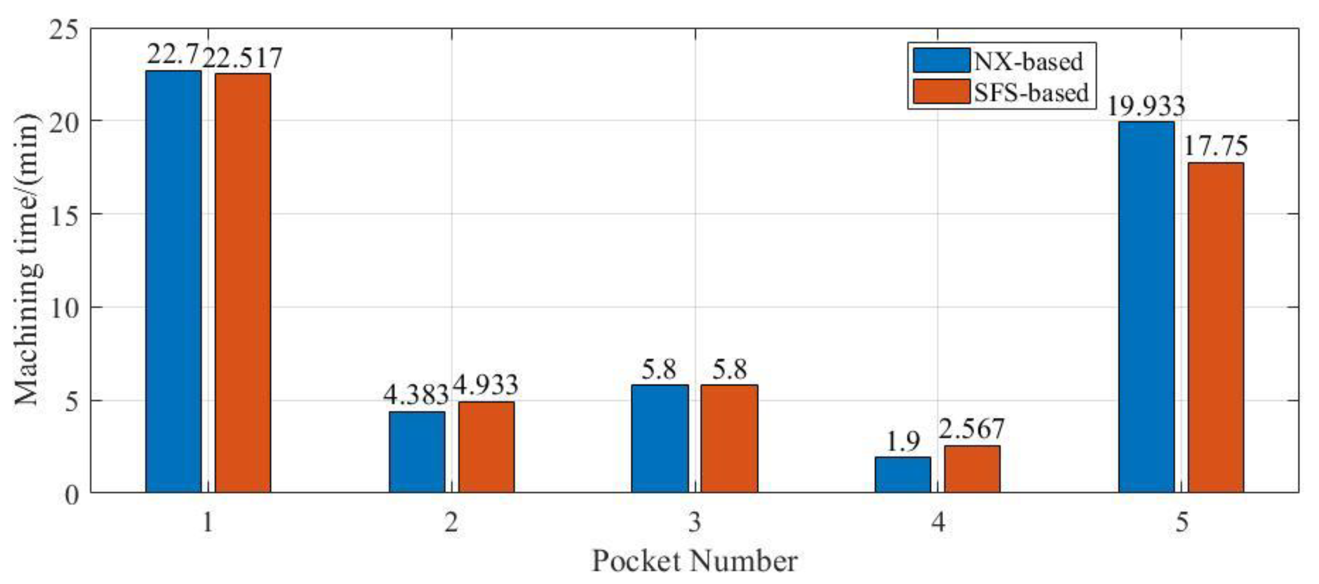
Pocket machining has been widely applied in the aerospace and mold industry. Although almost all commercial CAM packages provide the implementation of traditional strategy, the generated tool path is only based on the idea of geometric bias, which cannot simply and directly guarantee the high efficiency of the generated path. However, machining time is the most concerned evaluation index of tool path in roughing.
In this study, inspired by the phenomenon of sound field fluctuation and diffusion, a rough machining tool path generation method based on SFS is developed. The developed method is not only of great universality, but also has high machining efficiency, which is very suitable for rough machining of pockets. The specific generation method and process will be described in this section.
3.1. Medial Axis Transformation of Pocket
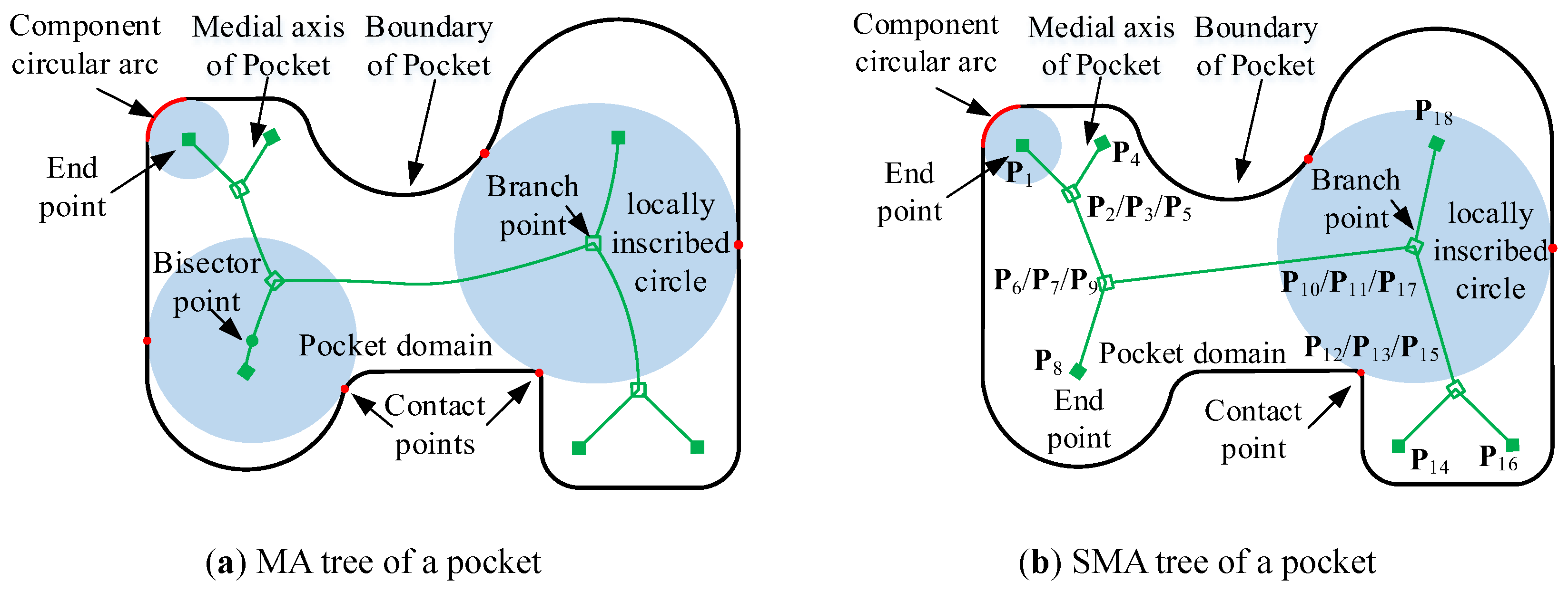
The medial axis transform (MAT) of a pocket is a completed shape descriptor, which is of great importance in describing the boundary of complex pocket [
22]. The MAT is based on medial axis (MA) and locally inscribed circles. The MA of the pocket is composed of all the locus of centers of the tangent circles, and it is also called the MA tree, as shown in
Figure 1a. The locally inscribed circles are confined to the boundary and can be placed anywhere in the pocket. A detailed description of MA can be found in literature [
22], including the definition of the locally inscribed circle, end point, bisector point, and branch point.
It is essential to calculate locally inscribed circles of bisector points accurately and efficiently in the calculation of MAT, and the method used in [
22] is directly used in this study. After that, the MAT should be stored in a tree data structure, and several specialized data structures have been developed in the past few years to represent the MA tree. In order to store the MA tree as simply as possible under the premise of application requirements, the strategy proposed in [
23] is adopted in this study and some adjustments are made to meet the requirements of the tool path generation method developed in this study.
In this method, complex MA tree structure is transformed into simple closed loop called the MA cycle by a clockwise or counterclockwise traversal strategy. The MA cycle begins at the MA point with the minimum locally tangent circle and visits the branch point more than twice, the bisector points twice, and the end point once.
Even though the MA consists of a series of curves that can be approximated by a series of linear segments, such a complex MA is not needed in the method of tool path generation in this study. Instead, only linear continuous secondary sources combined with the acoustic propagation method is needed to achieve the fitting of the straight line and curve boundary, which will be described in
Section 3.3. Therefore, after the calculation of MA, only branch points and end points are needed to construct a simplified MA (SMA), which can be marked as
. An example is shown in
Figure 1b, linear segments connecting branch points and end points are the simplified MA, which and can be represented by
. The Euclidean distance from
to
can be expressed as
.
3.2. Step-Over Calculation for Tool Path
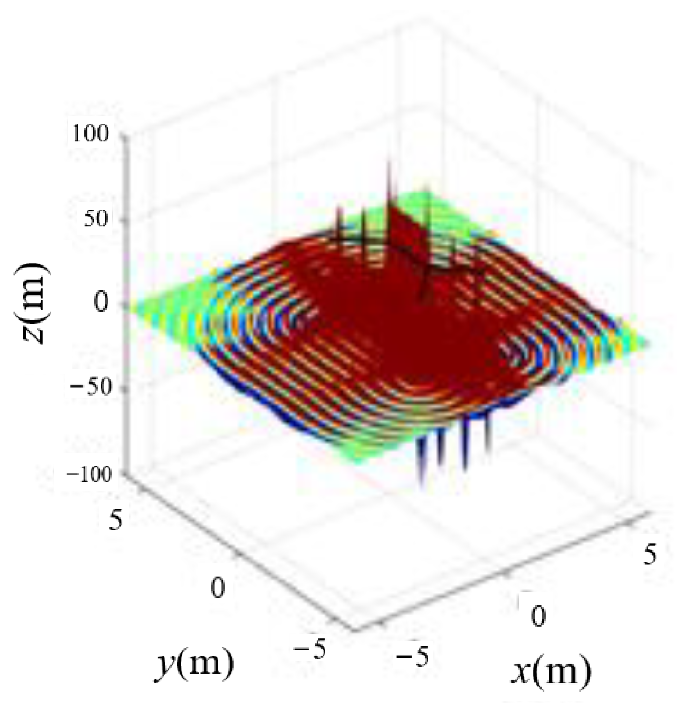
The first problem to be solved is to analyze the mapping between the step-over of the tool path and sound field parameters. It is not difficult to see that the mathematical description of the sound field caused by a plane wave in the time–frequency domain is a complex wave, which seems difficult to relate to the step-over. However, only the real part of it is used as the sound field in practical application, and the real part of Equation (1) can be expressed as
In this study, 2.5-D SFS is utilized in the generation of the tool path, however, if the theory of SFS is used for calculation, it is not difficult conclude that the calculation result is a wave surface by analyzing Equation (14), as shown in
Figure 2. It also shows that the diffusion process of the sound field is almost parallel and non-intersecting, which is very similar to the geometry of the cutting tool path.
To handle this problem, the intersection line of the surface and the x-y plane is used as the generated tool path, which means that the step-over between two adjacent tool paths is related to the wave cycle of the sound field and is half of the wave cycle in terms of spatial length. Therefore, the following relationship can be obtained by combining Equations (6) and (14)
which means the step-over of the tool path is determined by the time frequency and sound speed of the sound field, meaning that SFS can fully meet the actual needs of tool path generation.
3.3. Propagation Direction Calculation Considering Pocket Boundary Geometry
A SMA tree consisting of linear segments has been constructed in
Section 3.1 to generate the tool path by using continuous linear secondary sources. However, the SMA tree cannot reflect the geometric characteristics of the pocket boundary well, but instead only the segmentation of the boundary. Therefore, in order to make the synthesized sound field effectively reflect the geometric characteristics of the pocket boundary, different propagation directions of acoustic waves are studied to realize the matching of the synthetic sound field to different boundary features in this section.
3.3.1. Propagation Direction for Linear Boundary
The sound field solution method of linear secondary sources situated along the
x-axis and propagating to the
y-axis has been described in
Section 2, However, in order to use the linear sequences of SMA in
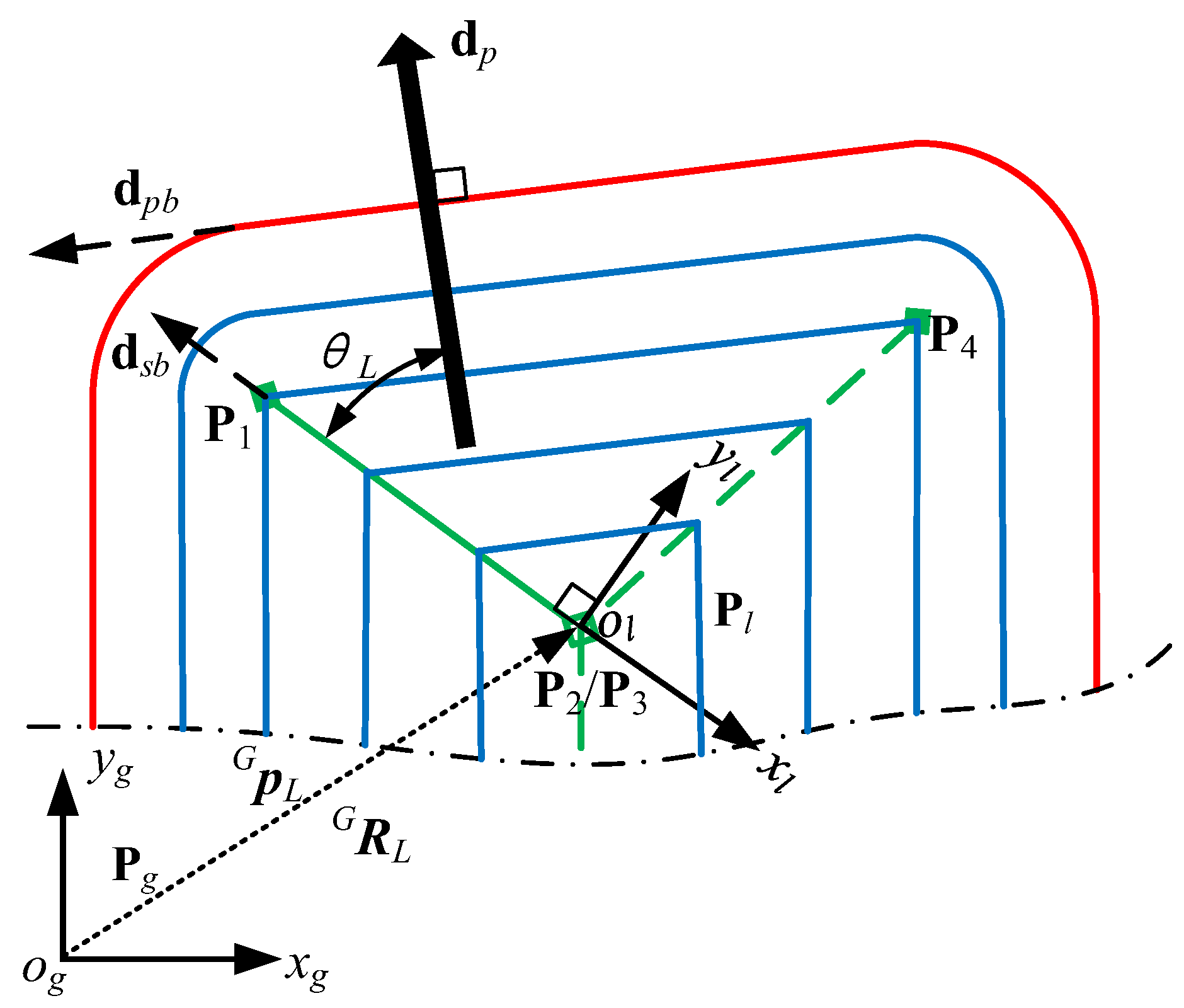
Section 3.1 to synthesize the sound field reflecting the comprehensive geometric characteristics of the pocket, the position and attitude of the secondary source must be transformed firstly, including translation and rotation. As shown in
Figure 3, the transformation of the secondary source position and attitude is described by taking the SMA
as an example, where
is the global coordinate of the pocket and
is the local coordinate of
. The transformation relationship is as follows
After the coordinate transformation, the propagation direction of each linear secondary source (segment of SMA) can be calculated in the local coordinates. Taking
to represent the propagation direction of
, and that the propagation direction is along the direction of
-axis if
. In order to meet the needs of different linear boundaries,
and
are utilized to represent the direction of linear boundary and the direction of the linear SMA, respectively, and then the propagation direction can be expressed as
where
denotes the angle between
and
.
An example of tool path generation based on the abovementioned method is shown in
Figure 4; it is not difficult to see the feasibility of the developed method and the advantage of smoothness at the corner.
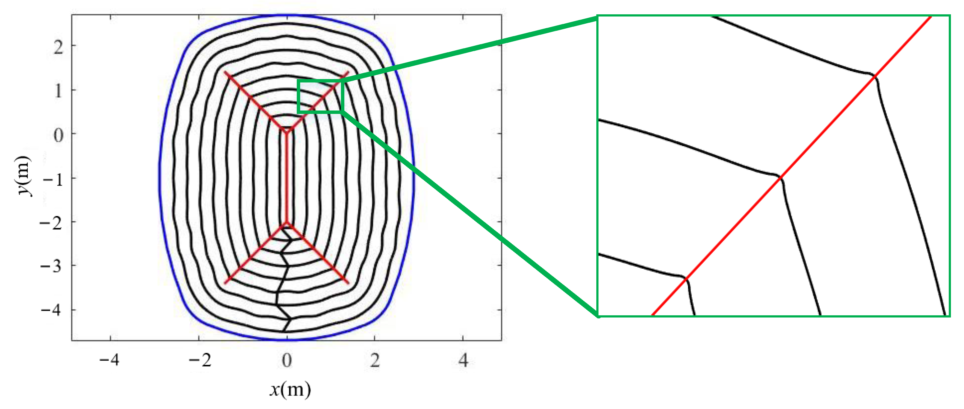
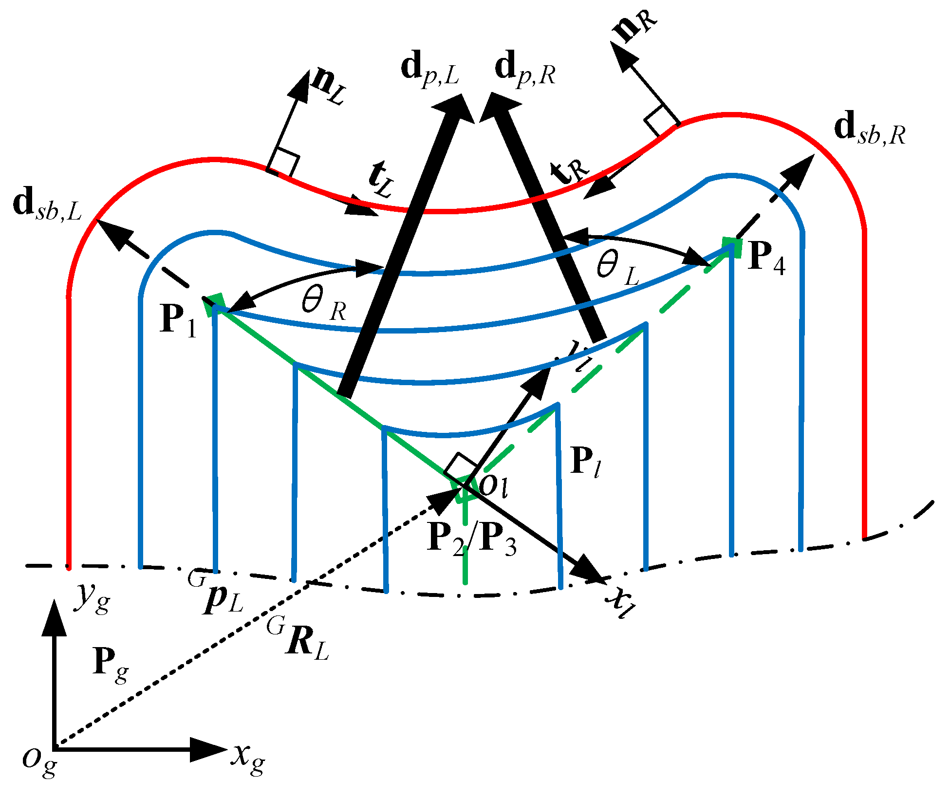
3.3.2. Propagation Direction for Convex Arc Boundary
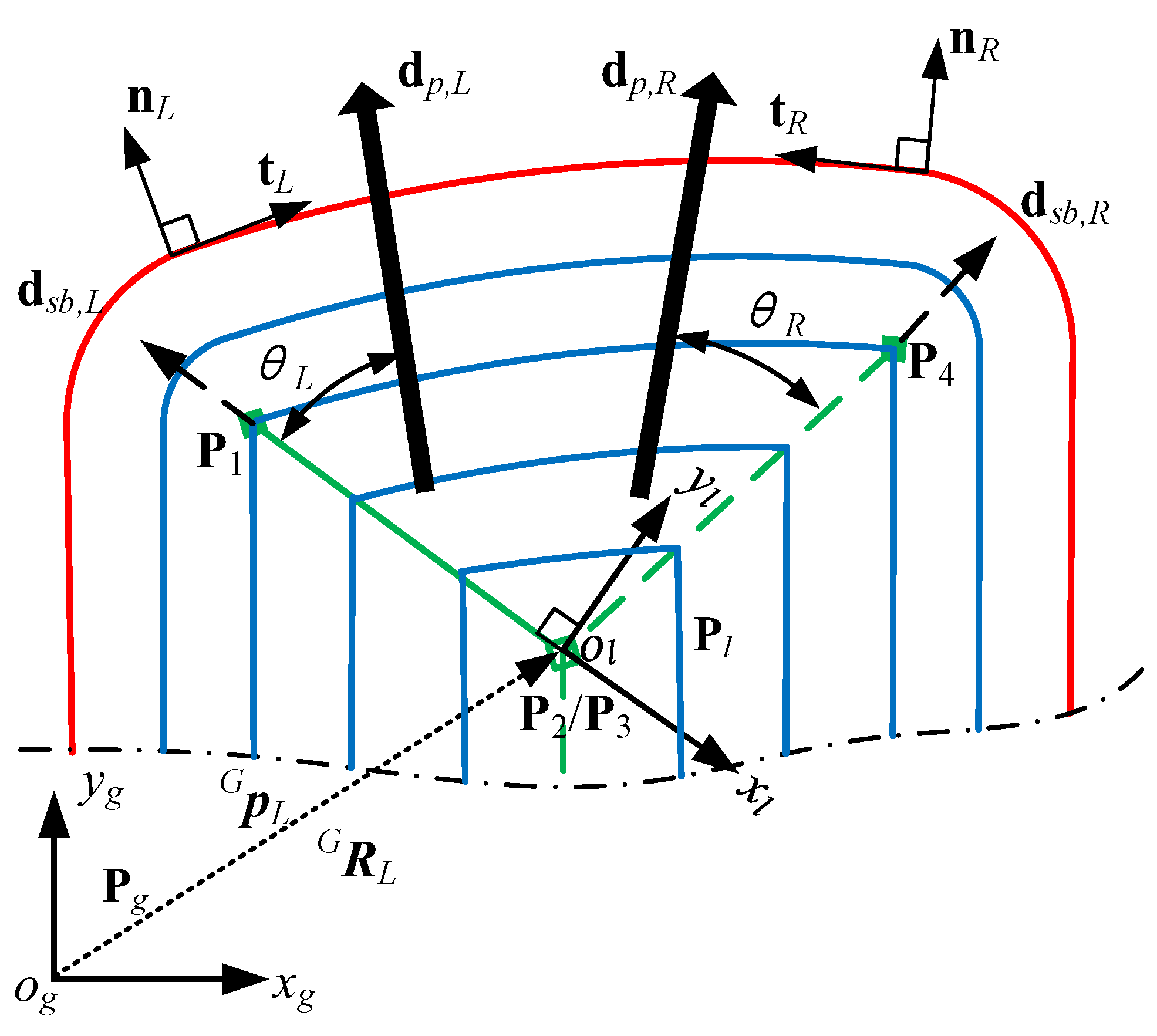
Analogous to the linear boundary, the propagation direction of each linear secondary source can be calculated in the local coordinates to approximate the convex arc boundary after the coordinate transformation, but the difference is that the approximation of a convex curve requires at least two linear secondary sources, as shown in
Figure 5. Taking
and
to represent the propagation direction of
and
, respectively, to meet the approximation of the convex arc boundary,
and
are utilized to represent the direction of linear SMA at the left and right, respectively. The normal vector and tangent vector of convex arc boundary at left and right ends of the curve can be expressed in turn as
,
,
and
, respectively, and the calculation of them are not complicated and will not be repeated here. After defining and calculating the above variables, the propagation direction of
and
can be expressed as
An example is also shown in
Figure 6; it is not difficult to see the feasibility of the developed method and the advantage of smoothness at the corner.
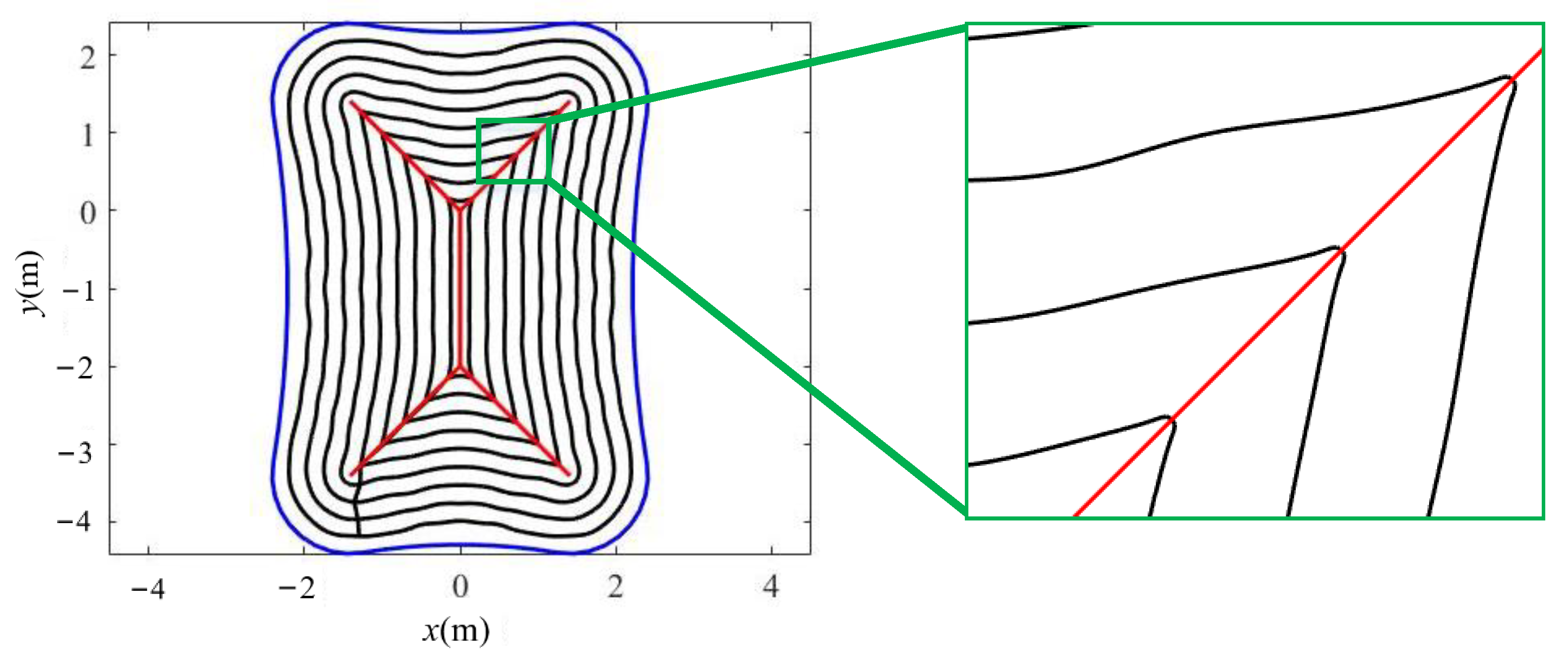
3.3.3. Propagation Direction for Concave Arc Boundary
The same as for the convex arc boundary, the propagation direction of each linear secondary source can be calculated in the local coordinates to approximate concave arc boundary after the coordinate transformation, as shown in
Figure 7. Taking
and
to represent the propagation direction of
and
, respectively, to meet the approximation of convex arc boundary,
and
are utilized to represent the direction of linear SMA at the left and right, respectively. The normal vector and tangent vector of convex arc boundary at left and right ends of the curve can be expressed in turn as
,
,
, and
, and the propagation direction of
and
can be expressed as
An example is also shown in
Figure 8; it is not difficult to see the feasibility of the developed method and the advantage of smoothness at the corner.
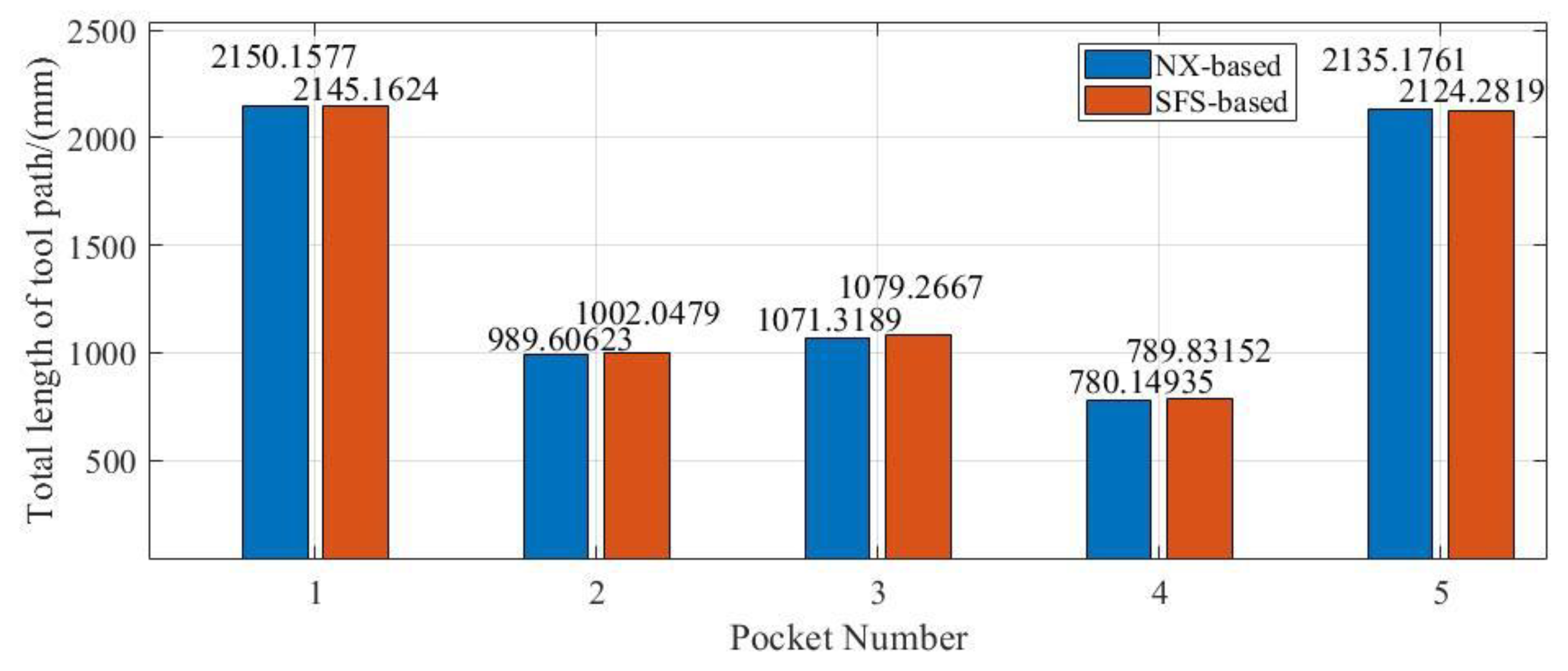
5. Conclusions
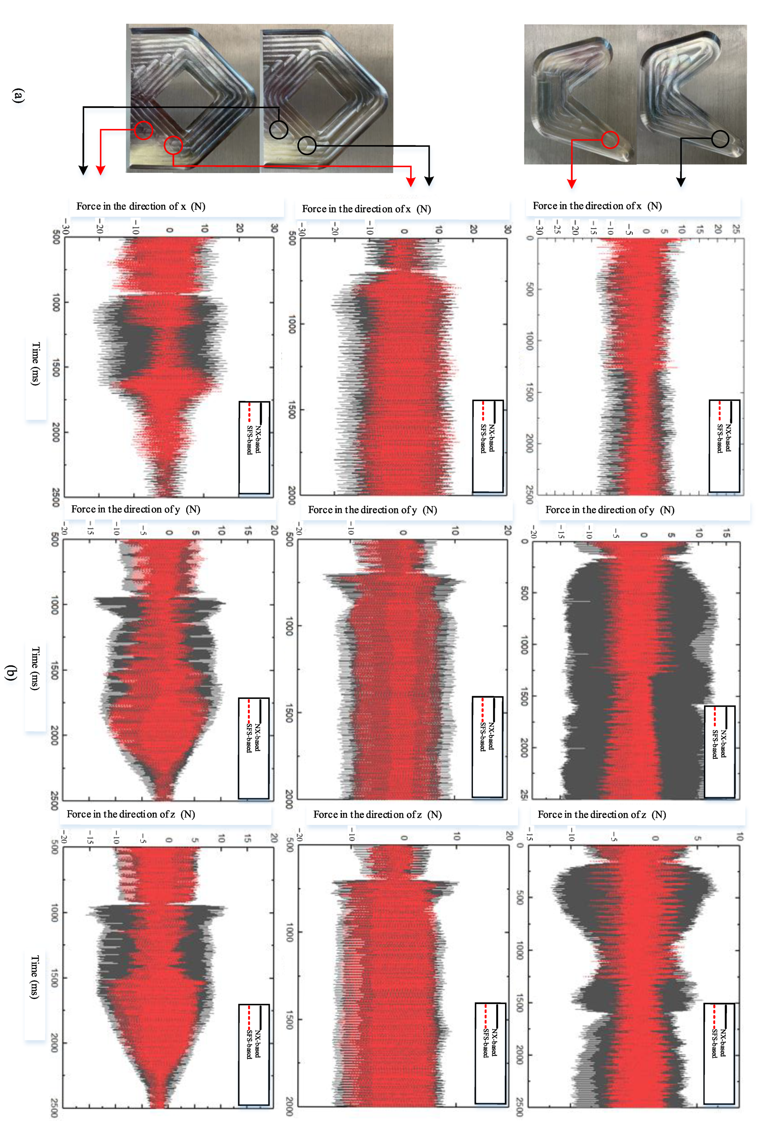
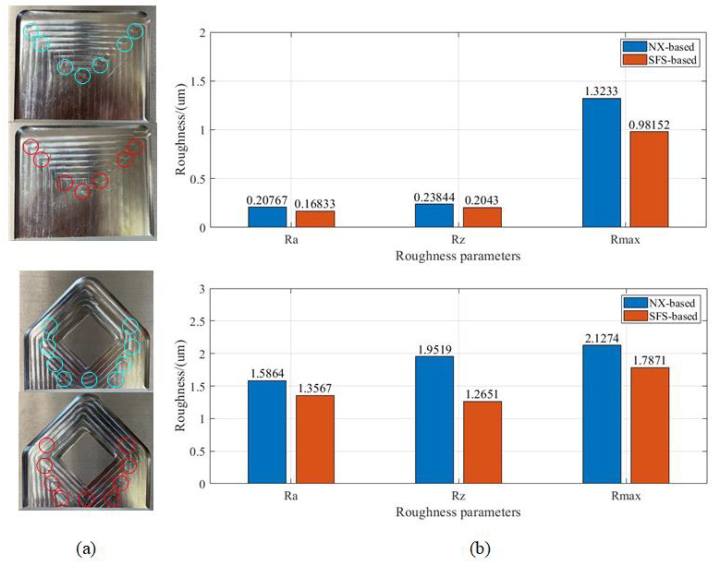
In this paper, a novel contoured parallel tool path generation method is developed. Compared to previous works, the SMA tree of the pocket is extracted in the proposed method and then the propagation direction of each SMA segment is calculated based on the geometric characteristics of the pocket boundary. Moreover, the final tool path is obtained through the synthesis of the sound field, which can not only match the geometry of the pocket boundary well, but also effectively achieves the goal of smoothness, no self-intersection, and no residual. Finally, the experimental results show that the tool path obtained by the developed SFS-based method has better advantages in smoothness, and the cutting force variation range during machining is much smaller, which reflected better dynamic performance. At the same time, the SFS-based method can effectively improve the machining quality and machining efficiency.
There is a research direction that deserves to be investigated in the future. Although this study is aimed at pocket milling, its idea can be extended to the milling of complex surfaces.


