Precise Dynamic Consensus under Event-Triggered Communication

Abstract

This work addresses the problem of dynamic consensus, which consists of estimating the dynamic average of a set of time-varying signals distributed across a communication network of multiple agents. This problem has many applications in robotics, with formation control and target tracking being some of the most prominent ones. In this work, we propose a consensus algorithm to estimate the dynamic average in a distributed fashion, where discrete sampling and event-triggered communication are adopted to reduce the communication burden. Compared to other linear methods in the state of the art, our proposal can obtain exact convergence under continuous communication even when the dynamic average signal is persistently varying. Contrary to other sliding-mode approaches, our method reduces chattering in the discrete-time setting. The proposal is based on the discretization of established exact dynamic consensus results that use high-order sliding modes. The convergence of the protocol is verified through formal analysis, based on homogeneity properties, as well as through several numerical experiments. Concretely, we numerically show that an advantageous trade-off exists between the maximum steady-state consensus error and the communication rate. As a result, our proposal can outperform other state-of-the-art approaches, even when event-triggered communication is used in our protocol.

1. Introduction

The problem of dynamic consensus, also referred to as dynamic average tracking, consists of computing the average of a set of time-varying signals distributed across a communication network. This problem has recently attracted a lot of attention due to its applications in general cyber-physical systems and robotics. For instance, dynamic consensus algorithms can be used to coordinate multi-robot systems, formation control, and target tracking, as in [1,2]. A more detailed overview of the common problems in the field of multi-robot coordination can be found in [3].

Many dynamic consensus approaches in continuous time exist in the literature [4]. For example, a high-order linear dynamic consensus approach is proposed in [5], which is capable of achieving arbitrarily small steady-state errors when persistently varying signals are used by tuning a protocol parameter. The protocol in [6] adopts a similar linear approach and analyses its performance against bounded cyber-attacks in the communication network. In [7], another linear consensus protocol is proposed to address the problem of having active and passive sensing nodes with time-varying roles. While these approaches obtain good theoretical results in continuous time, only discrete-time communication is possible in practice. In contrast, other works are designed directly in a discrete-time setting where local time-varying signals are sampled with a fixed sampling step shared across the network. For example, a high-order discrete-time linear dynamic consensus algorithm is proposed in [8] with similar performance to those in continuous time. The proposal in [9] extends the previous work to ensure it is robust to initialization errors. Similar ideas are applied to distributed convex optimization in [10].

Besides having discrete communication, maintaining a low communication burden in the network is desirable, both from power consumption and communication bandwidth usage perspectives. For this purpose, an event-triggered approach can be used to decide when agents should communicate instead of doing so at every sampling instant. Several works use event-triggered conditions in which the estimate for the average signal for a particular agent is only shared when it changes sufficiently with respect to the last transmitted value. For example, an event-triggered communication rule is applied to a continuous-time dynamic consensus problem in [11]. In [12], an event-triggered dynamic consensus approach is analysed for homogeneous and heterogeneous multi-agent systems. These ideas have shown to be helpful in distributed state estimation. For instance, deterministic [13] and stochastic [14] event-triggering rules have been used to construct distributed Kalman filters. The proposal in [15] borrows these ideas to construct an extended Kalman filter. Distributed set-membership estimators have also been studied in the context of event-triggered communication [16]. Event-triggered schemes for estimation typically result in a trade-off between the quality of the estimates and the number of triggered communication events, as is pointed out in [17]. This allows the user to tune the parameters of the event-triggering condition to reduce communication while achieving a desired estimation error for the consensus estimates. A more in-depth look into event-triggered strategies can be found in [18].

However, most event-triggered and discrete-time approaches for dynamic consensus are based on linear techniques, even in recent works [15]. This means that the estimations cannot be exact when the dynamic average is persistently varying, e.g., when the local signals behave as a sinusoidal. Concretely, these approaches typically attain a bounded steady-state error, which can become arbitrarily small by increasing some parameters in the algorithm [4]. Despite this, as typical with high-gain arguments, increasing such parameters can reduce the algorithm’s robustness when only imperfect measurements or noisy local signals are available [19]. In contrast, exact dynamic consensus algorithms can achieve exact convergence towards the dynamic average under reasonable assumptions for the local signals, including the persistently varying case. For example, a discontinuous First-Order Sliding Mode (FOSM) approach is used in [20] to achieve exact convergence in this setting. Similar ideas are applied in [21] for continuous-time state estimation. The work in [22] proposes a High-Order Sliding Mode (HOSM) approach for exact dynamic consensus, which was then extended in [23] to account for initialization errors. Note that these approaches are mainly based on sliding modes to achieve such an exact convergence. As a result, continuous-time analysis is mostly available for these protocols.

Unfortunately, sliding modes deteriorate their performance in the discrete-time setting due to the so-called chattering ([24], Chapter 3). In particular, FOSM approaches for dynamic consensus in [20,21] deteriorate its performance in an order proportional to the time step in the discrete-time setting. A standard solution to attenuate chattering is to use HOSM [24]. To the best of our knowledge, the only methods that use HOSM for dynamic consensus are [22,23]. However, discrete-time analysis or event-triggered extensions for these approaches have not been discussed so far in the literature.

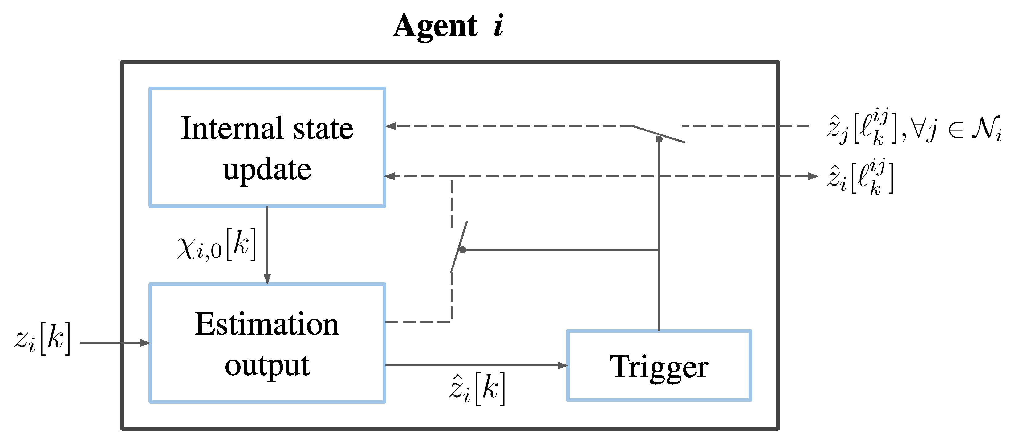
As a result of this discussion, we contribute a novel distributed dynamic consensus algorithm with the following features. First, the algorithm uses discrete-time samples of the local signal. We also propose the adoption of event-triggered communication between agents to reduce the communication burden. Our proposal is consistently exact, which means that the exact estimation of the average signal is obtained when the time step approaches zero and when events are triggered at each sampling step. We show the advantage of our method against linear approaches, in which the permanent consensus error cannot be eliminated. Moreover, in the general discrete-time case, we show that our proposal reduces chattering when compared to exact FOSM approaches.

This article is organized as follows. Section 2 provides a description of the problem of interest and our proposal to solve the consensus problem on a discrete-time setting using event-triggered communication. A formal analysis of the convergence for our protocol can be found in Section 3. In Section 4, we validate our proposal and compare it to other methods through simulation experiments. Furthermore, Section 5 provides a qualitative discussion comparing our proposal to other related works. The conclusions and future work are drawn in Section 6.

2. Problem Statement and Protocol Proposal

In this Section, we describe the problem of interest and our proposed consensus protocol to solve it using event-triggered communication between the agents.

2.1. Notation

Let $\mathbf{x}={[x_1,\cdots ,x_n]}^{\top }\in {\mathbb{R}}^n$, then ${\parallel \mathbf{x}\parallel }_{\infty }:=max{\left\{x_i\right\}}_{i=1}^n$. Let $𝟙={[1,\cdots ,1]}^{\top }\in {\mathbb{R}}^n$, $\mathbf{U}=𝟙{𝟙}^{\top }$ the matrix with unit elements and ${\mathbf{I}}_n\in {\mathbb{R}}^{n\times n}$ the identity matrix. Let $\mathrm{sign}\left(x\right)=1$ if $x>0, \mathrm{sign}\left(x\right)=-1$ if $x<0$ and $\mathrm{sign}\left(0\right)=0$. Moreover, if $x\in \mathbb{R}$, let ${\lceil x\rfloor }^{\alpha }:={\left|x\right|}^{\alpha }\mathrm{sign}\left(x\right)$ for $\alpha >0$ and ${\lceil x\rfloor }^0:=\mathrm{sign}\left(x\right)$. When $\mathbf{x}={[x_1,\cdots ,x_n]}^{\top }\in {\mathbb{R}}^n$, then ${⌈\mathbf{x}⌋}^{\alpha }:={\left[{⌈x_1⌋}^{\alpha },\cdots ,{⌈x_n⌋}^{\alpha }\right]}^{\top }$ for $\alpha \ge 0$. Let $x^{\left(n\right)}$ represent the nth order derivative of x. The notation $c[-1,1]$, with some $c\in \mathbb{R}$, refers to the interval $[-c,c]$.

2.2. Problem Statement

Consider a multi-agent system distributed in a network $\mathcal{G}=(\mathcal{V},\mathcal{E})$ with node set $\mathcal{V}=\{1,\cdots ,\mathsf{N}\}$ and edge set $\mathcal{E}\subseteq \mathcal{V}\times \mathcal{V}$, modelling communication links between agents. In the following, $\mathcal{G}$ is an undirected connected graph of $\mathsf{N}$ agents characterised by an adjacency matrix $\mathbf{A}$ and equally described by an incidence matrix $\mathbf{D}$, choosing an arbitrary orientation ([25], Chapter 8). Let ${\mathcal{N}}_i$ denote the index set of neighbours for an agent $i\in \mathcal{V}$.

We consider that each agent $i\in \mathcal{V}$ has access to a local time-varying signal $z_i\left(t\right)\in \mathbb{R}$ at some fixed sampling instants $t\in {\{k\Delta \}}_{k=0}^{\infty }$ where $\Delta$ is the sampling period. We write $z_i\left[k\right]:=z_i(k\Delta )$ for simplicity. The goal is for all the agents to estimate the dynamic average signal [4]:

$$\overline{z}\left(t\right)=\frac{1}{\mathsf{N}}\sum _{i=1}^{\mathsf{N}}{z}_i\left(t\right)$$

(1)

in a distributed fashion, by sharing information between them.

2.3. Protocol Proposal

Our proposal to solve the multi-agent consensus problem is a protocol that adopts event-triggered communication to reduce the communication burden in the network of agents. It also uses High-Order Sliding Modes to achieve precise consensus results.

Event-triggered communication: To reduce the communication burden in the network, an event-triggered approach is used to decide when an agent communicates with its neighbours. Denote with ${\widehat{z}}_i\left[k\right]$ the estimation that agent $i\in \mathcal{V}$ has for the signal $\overline{z}\left(t\right)$ at $t=k\Delta$. Then, the communication link $(i,j)\in \mathcal{E}$ is updated at the sequence of instants ${\left\{{\ell }_k^{ij}\right\}}_{k=0}^{\infty }$ provided by the recursive triggering rule:

$${\ell }_k^{ij}=\left\{\begin{array}{cc}k\hfill & \mathrm{if}|{\widehat{z}}_i\left[k\right]-{\widehat{z}}_i\left[{\ell }_{k-1}^{ij}\right]|\ge \epsilon \vee |{\widehat{z}}_j\left[k\right]-{\widehat{z}}_j\left[{\ell }_{k-1}^{ij}\right]|\ge \epsilon \hfill \\ {\ell }_{k-1}^{ij}\hfill & \mathrm{otherwise}\hfill \end{array}\right.$$

(2)

where $\epsilon \ge 0$ is a design parameter and by setting ${\ell }_0^{ij}=0$ without loss of generality. The interpretation of (2) is that both agents $i,j$ for a link $(i,j)\in \mathcal{E}$ have stored local copies of each other’s estimation ${\widehat{z}}_i\left[{\ell }_{k-1}^{ij}\right],{\widehat{z}}_j\left[{\ell }_{k-1}^{ij}\right]$ from the last time the link was updated. If agent i detects that its current estimation ${\widehat{z}}_i\left[k\right]$ satisfies $|{\widehat{z}}_i\left[k\right]-{\widehat{z}}_i\left[{\ell }_{k-1}^{ij}\right]|\ge \epsilon$, it then sends ${\widehat{z}}_i\left[k\right]$ to agent j, which responds by sending its current estimation ${\widehat{z}}_j\left[k\right]$ back. Subsequently, both agents update ${\ell }_k^{ij}=k$. A similar protocol occurs when agent j detects $|{\widehat{z}}_j\left[k\right]-{\widehat{z}}_j\left[{\ell }_{k-1}^{ij}\right]|\ge \epsilon$.

The proposed algorithm to estimate $\overline{z}\left(t\right)$ in this setting is of the following form. Each agent $i\in \{1,\cdots ,\mathsf{N}\}$ has $m+1$ internal states ${\mathsf{\chi }}_{i,0}\left[k\right],\cdots ,{\mathsf{\chi }}_{i,m}\left[k\right]$ from which the local estimation ${\widehat{z}}_i\left[k\right]$ is computed according to:

$$\begin{array}{cc}\hfill & \mathbf{Internal}\mathbf{state}\mathbf{update}:\hfill \\ \hfill & \begin{array}{cc}\hfill {\mathsf{\chi }}_{i,\mu }[k+1]& {\displaystyle =\sum _{\nu =0}^{m-\mu }\left(\frac{{\Delta }^{\nu }}{\nu !}\right){\mathsf{\chi }}_{i,\mu +\nu }\left[k\right]+\Delta g_{\mu }\sum _{j\in {\mathcal{N}}_i}{F}_{\mu }\left({\widehat{z}}_i\left[{\ell }_k^{ij}\right]-{\widehat{z}}_j\left[{\ell }_k^{ij}\right]\right),}\hfill \\ \hfill & \mathrm{for}\mu \in \{0,\cdots ,m-1\}\hfill \\ \hfill {\mathsf{\chi }}_{i,m}[k+1]& {\displaystyle ={\mathsf{\chi }}_{i,m}\left[k\right]+\Delta g_m\sum _{j\in {\mathcal{N}}_i}{F}_m\left({\widehat{z}}_i\left[{\ell }_k^{ij}\right]-{\widehat{z}}_j\left[{\ell }_k^{ij}\right]\right),}\hfill \end{array}\hfill \\ \hfill & \mathbf{Estimation}\mathbf{output}:\hfill \\ \hfill & \begin{array}{cc}\hfill {\widehat{z}}_i\left[k\right]& :=z_i\left[k\right]-{\mathsf{\chi }}_{i,0}\left[k\right]\hfill \end{array}\hfill \end{array}$$

(3)

with gains $g_0,\cdots ,g_m>0$ and $F_{\mu }(•)={⌈•⌋}^{\frac{m-\mu }{m+1}}$. The proposal for the exact dynamic consensus algorithm with the event-triggered communication between the agents is summarized in Algorithm 1. Figure 1 illustrates the flow of information for each agent $i\in \mathcal{V}$.    

Algorithm 1: Exact dynamic consensus with event-triggered communication

To ensure the convergence of (3), we require the following assumption for the signals $z_i\left(t\right)$, regardless of the sampling period $\Delta$:

Assumption A1.

Given $L>0$, then it follows that:

$$\left|{\overline{z}}^{(m+1)}\left(t\right)-z_i^{(m+1)}\left(t\right)\right|\le L,\forall t\ge 0$$

Theorem 1.

Let $\mathcal{G}$ be a connected graph and Assumption 1 hold for some fixed $L>0$. Then, for any $\Delta ,\epsilon >0$ there exist sufficiently high gains $g_0,\cdots ,g_m$ and some $K\in \mathbb{N}$, such that if ${\sum }_{i=1}^{\mathsf{N}}{\mathsf{\chi }}_{i,\mu }\left[0\right]=0,\forall \mu \in \{0,\cdots ,m\}$ then:

$$|{\widehat{z}}_i\left[k\right]-\overline{z}\left[k\right]|\le cmax\{{\Delta }^{m+1},\epsilon \sqrt{\mathsf{N}}\},\forall k\ge K$$

for some constant $c>0$.

The condition ${\sum }_{i=1}^{\mathsf{N}}{\mathsf{\chi }}_{i,\mu }\left[0\right]=0$ in the previous theorem has been used in other works in the literature [4,22] and is complied trivially by setting ${\mathsf{\chi }}_{i,\mu }\left[0\right]=0$. The proof for Theorem 1 is provided in Section 3.1.

In addition, if samples of the derivatives $z_i^{\left(\mu \right)}\left[k\right],\mu \in \{0,\cdots ,m\}$ are also available, either by assumption or through a differentiation algorithm [26], then additional outputs can be obtained as:

$${\widehat{z}}_{i,\mu }\left[k\right]:=z_i^{\left(\mu \right)}\left[k\right]-{\mathsf{\chi }}_{i,\mu }\left[k\right]$$

(4)

which estimate the derivatives ${\left\{{\overline{z}}^{\left(\mu \right)}\left(t\right)\right\}}_{\mu =0}^m$ at $t=k\Delta$. The following result regarding the outputs (4) is obtained as a consequence of the proof of Theorem 1 in Section 3.1.

Corollary 1.

Consider the assumptions of Theorem 1 and the outputs in (4). Then, in addition to the conclusion of Theorem 1, there also exist $c_0,\cdots ,c_{\mu }>0$ such that:

$$|{\widehat{z}}_{i,\mu }\left[k\right]-{\overline{z}}^{\left(\mu \right)}\left[k\right]|\le c_{\mu }max\left\{{\Delta }^{m-\mu +1},{\left(\epsilon \sqrt{\mathsf{N}}\right)}^{\frac{m-\mu +1}{m+1}}\right\}$$

Remark 1.

While the performance of our proposal in (3) is not exact as a result of Theorem 1, we say that it is consistently exact. This means that the exact convergence is obtained when $(\Delta ,\epsilon )\to (0,0)$, even under persistently varying local signals ${\left\{z_i\left(t\right)\right\}}_{i=1}^{\mathsf{N}}$, recovering the performance of the continuous-time protocol in [22].

Remark 2.

Note that if $m=0$, our proposal in (3) is similar to the approaches in [20,21], which use FOSM. In this case, considering $\epsilon =0$, the error bound performance of the protocol is proportional to Δ as a result of Theorem 1, as expected due to chattering. Moreover, by increasing the order $m>0$ of the sliding modes in (3), the effect of chattering is attenuated by having an error bound performance proportional to ${\Delta }^{m+1}$, which is smaller than Δ for small sampling steps.

Remark 3.

In light of Theorem 1 and Corollary 1, it can be concluded that the event-triggering threshold ε affects the maximum error bound. Hence, its value can be tuned for a particular application according to the magnitude of the admissible consensus error. Moreover, recalling (2), the parameter ε represents the admissible error one node can have in its knowledge of its neighbours’ estimates. For this reason, ε should be small enough to guarantee that the magnitude of the difference $|{\widehat{z}}_i\left[k\right]-{\widehat{z}}_i\left[{\ell }_{k-1}^{ij}\right]|$ is acceptable in comparison to the amplitude of the signal ${\overline{z}}_i\left(t\right)$ according to the application requirements.

Remark 4.

Theorem 1 ensures the existence of sufficiently high gains $g_0,\cdots ,g_m$ such that the convergence of (3) is obtained. However, the proof of the theorem reveals that these gains can be extracted precisely from a continuous-time EDCHO protocol. Hence, we refer the reader to [22], where a design procedure for the EDCHO gains $g_0,\cdots ,g_m$ is described in detail based on well-established techniques.

3. Protocol Convergence

In this Section, we provide a formal analysis of the convergence of our consensus protocol. To do so, we introduce three technical lemmas before providing the proof of Theorem 1 in Section 3.1.

First, define ${\mathsf{\chi }}_{\mu }\left[k\right]={[{\mathsf{\chi }}_{i,0}\left[k\right],\cdots ,{\mathsf{\chi }}_{i,m}\left[k\right]]}^{\top }$ and $\mathbf{z}\left(t\right)={[z_1\left(t\right),\cdots ,z_{\mathsf{N}}\left(t\right)]}^{\top }$. Moreover, define:

$${\widehat{z}}_{i,\mu }\left[k\right]=z_i^{\left(\mu \right)}\left[k\right]-{\mathsf{\chi }}_{i,\mu }\left[k\right]$$

where ${\widehat{z}}_i\left[k\right]\equiv {\widehat{z}}_{i,0}\left[k\right]$, as well as ${\widehat{\mathbf{z}}}_{\mu }\left[k\right]={[{\widehat{z}}_{1,\mu }\left[k\right],\cdots ,{\widehat{z}}_{\mathsf{N},\mu }\left[k\right]]}^{\top }$. In addition, note that ${\widehat{z}}_i\left[k\right]={\widehat{z}}_i\left[{\ell }_k^{ij}\right]+{\epsilon }_i\left[k\right]$ where $|{\epsilon }_i\left[k\right]|\le \epsilon$ by construction from (2). Hence, ${\widehat{\mathbf{z}}}_0\left[{\ell }_k^{ij}\right]={\widehat{\mathbf{z}}}_0\left[k\right]-\mathbf{\epsilon }\left[k\right]$ with $\mathbf{\epsilon }\left[k\right]={[{\epsilon }_1\left[k\right],\cdots ,{\epsilon }_{\mathsf{N}}\left[k\right]]}^{\top }$ and $\parallel \mathbf{\epsilon }\left[k\right]\parallel \le \epsilon \sqrt{\mathsf{N}}$.

Thus, the protocol in (3) can be written in vector form as:

$$\begin{array}{cc}\hfill {\mathsf{\chi }}_{\mu }[k+1]& =\sum _{\nu =0}^{m-\mu }\left(\frac{{\Delta }^{\nu }}{\nu !}\right){\mathsf{\chi }}_{\mu +\nu }\left[k\right]+\Delta g_{\mu }\mathbf{D}{⌈{\mathbf{D}}^{\top }({\widehat{\mathbf{z}}}_0\left[k\right]-\mathbf{\epsilon }\left[k\right])⌋}^{\frac{m-\mu }{m+1}}\hfill \\ \hfill {\mathsf{\chi }}_m[k+1]& ={\mathsf{\chi }}_m\left[k\right]+\Delta g_m\mathbf{D}{⌈{\mathbf{D}}^{\top }({\widehat{\mathbf{z}}}_0\left[k\right]-\mathbf{\epsilon }\left[k\right])⌋}^0\hfill \end{array}$$

(5)

for which the condition ${\sum }_{i=1}^{\mathsf{N}}{\mathsf{\chi }}_{i,\mu }\left[0\right]=0$ in Theorem 1 can be written as ${𝟙}^{\top }{\mathsf{\chi }}_{\mu }\left[0\right]=0$.

The purpose of the internal variables ${\mathsf{\chi }}_{\mu }\left[k\right]$ is to approximate the disagreement between local signals expressed as $\mathbf{P}{\mathbf{z}}^{\left(\mu \right)}\left[k\right]$ with $\mathbf{P}={\mathbf{I}}_{\mathsf{N}}-(1/\mathsf{N})\mathbf{U}$ recalling that $\mathbf{U}=𝟙{𝟙}^{\top }$ such that if ${\mathsf{\chi }}_{\mu }\left[k\right]=\mathbf{P}{\mathbf{z}}^{\left(\mu \right)}\left[k\right]$ exactly, then all the agents reach consensus towards:

$${\widehat{\mathbf{z}}}_{\mu }\left[k\right]={\mathbf{z}}^{\left(\mu \right)}\left[k\right]-{\mathsf{\chi }}_{\mu }\left[k\right]=(1/\mathsf{N})\mathbf{U}{\mathbf{z}}^{\left(\mu \right)}\left[k\right]=𝟙{\overline{z}}^{\left(\mu \right)}\left[k\right]$$

The first step to show that ${\mathsf{\chi }}_{\mu }\left[k\right]$ approximates $\mathbf{P}{\mathbf{z}}^{\left(\mu \right)}\left[k\right]$ is showing that it is always orthogonal to the consensus direction in the following result.

Lemma 1.

Let $\mathcal{G}$ be connected and ${𝟙}^{\top }{\mathsf{\chi }}_{\mu }\left[0\right]=0$ hold $\forall \mu \in \{0,\cdots ,m\}$. Then, (5) satisfies ${𝟙}^{\top }{\mathsf{\chi }}_{\mu }\left[k\right]=0,\forall k\ge 0,\forall \mu \in \{0,\cdots ,m\}$.

Proof. 

The proof follows by strong induction. Note that, ${𝟙}^{\top }{\mathsf{\chi }}_m[k+1]={𝟙}^{\top }{\mathsf{\chi }}_m\left[k\right]$ from (5) since ${𝟙}^{\top }\mathbf{D}=\mathbf{0}$. Hence, ${𝟙}^{\top }{\mathsf{\chi }}_m\left[k\right]=0,\forall k\ge 0$ due to the initial condition ${𝟙}^{\top }{\mathsf{\chi }}_m\left[0\right]=0$. Now, use this as an induction base for the rest of the $\mu \in \{1,\cdots ,m-1\}$. Assume from the induction hypothesis that ${𝟙}^{\top }{\mathsf{\chi }}_{\mu +\nu }\left[k\right]=0,\forall k\ge 0$ with $\nu \in \{1,\cdots ,m-\mu \}$ and $\mu <m$. Then, from (5):

$${𝟙}^{\top }{\mathsf{\chi }}_{\mu }[k+1]={𝟙}^{\top }{\mathsf{\chi }}_{\mu }\left[k\right]+\sum _{\nu =1}^{m-\mu }\left(\frac{{\Delta }^{\nu }}{\nu !}\right){𝟙}^{\top }{\mathsf{\chi }}_{\mu +\nu }\left[k\right]={𝟙}^{\top }{\mathsf{\chi }}_{\mu }\left[k\right]$$

from which it follows that ${𝟙}^{\top }{\mathsf{\chi }}_{\mu }\left[k\right]=0,\forall k\ge 0$ similarly as before, completing the proof. □

Now, let the error ${\tilde{\mathsf{\chi }}}_{\mu }\left[k\right]={\mathsf{\chi }}_{\mu }\left[k\right]-\mathbf{P}{\mathbf{z}}^{\left(\mu \right)}\left[k\right]$ and recall from Corollary A2 in Appendix B that ${\tilde{\mathbf{z}}}^{\left(\mu \right)}\left[k\right]=\mathbf{P}{\mathbf{z}}^{\left(\mu \right)}\left[k\right]$ can be expanded as:

$${\tilde{\mathbf{z}}}^{\left(\mu \right)}[k+1]=\sum _{\nu =0}^{m-\mu }\left(\frac{{\Delta }^{\nu }}{\nu !}\right){\tilde{\mathbf{z}}}^{(\mu +\nu )}\left[k\right]+{\mathbf{r}}_{\mu }\left[k\right]$$

(6)

where ${\mathbf{r}}_{\mu }\left[k\right]\in ({\Delta }^{m-\mu +1}/(m-\mu +1)!){[-L,L]}^{\mathsf{N}}$. Therefore, combining (5) and (6), the error dynamics for ${\tilde{\mathsf{\chi }}}_{\mu }\left[k\right]$ can be written as:

$$\begin{array}{cc}\hfill {\tilde{\mathsf{\chi }}}_{\mu }[k+1]& =\sum _{\nu =0}^{m-\mu }\left(\frac{{\Delta }^{\nu }}{\nu !}\right){\tilde{\mathsf{\chi }}}_{\mu +\nu }\left[k\right]-\Delta g_{\mu }\mathbf{D}{⌈{\mathbf{D}}^{\top }({\tilde{\mathsf{\chi }}}_0\left[k\right]+\mathbf{\epsilon }\left[k\right])⌋}^{\frac{m-\mu }{m+1}}+{\mathbf{r}}_{\mu }\left[k\right]\hfill \\ \hfill {\tilde{\mathsf{\chi }}}_m[k+1]& ={\tilde{\mathsf{\chi }}}_m\left[k\right]-\Delta g_m\mathbf{D}{⌈{\mathbf{D}}^{\top }({\tilde{\mathsf{\chi }}}_0\left[k\right]+\mathbf{\epsilon }\left[k\right])⌋}^0+{\mathbf{r}}_m\left[k\right]\hfill \end{array}$$

(7)

using ${\mathbf{D}}^{\top }({\widehat{\mathbf{z}}}_0\left[k\right]-\mathbf{\epsilon }\left[k\right])=-{\mathbf{D}}^{\top }({\tilde{\mathsf{\chi }}}_0\left[k\right]+\mathbf{\epsilon }\left[k\right])$ due to ${\mathbf{D}}^{\top }={\mathbf{D}}^{\top }\mathbf{P}$. Rearranging (7) leads to:

$$\begin{array}{cc}\hfill {\tilde{\mathsf{\chi }}}_{\mu }[k+1]& ={\tilde{\mathsf{\chi }}}_{\mu }\left[k\right]+\Delta (\sum _{\nu =1}^{m-\mu }\left(\frac{{\Delta }^{\nu -1}}{\nu !}\right){\tilde{\mathsf{\chi }}}_{\mu +\nu }\left[k\right]\hfill \\ & -g_{\mu }\mathbf{D}{⌈{\mathbf{D}}^{\top }({\tilde{\mathsf{\chi }}}_0\left[k\right]+\mathbf{\epsilon }\left[k\right])⌋}^{\frac{m-\mu }{m+1}}+{\mathbf{r}}_{\mu }\left[k\right]/\Delta )\hfill \\ \hfill {\tilde{\mathsf{\chi }}}_m[k+1]& ={\tilde{\mathsf{\chi }}}_m\left[k\right]+\Delta \left(-g_m\mathbf{D}{⌈{\mathbf{D}}^{\top }({\tilde{\mathsf{\chi }}}_0\left[k\right]+\mathbf{\epsilon }\left[k\right])⌋}^0+{\mathbf{r}}_m\left[k\right]/\Delta \right)\hfill \end{array}$$

(8)

Hence, all trajectories of (8) satisfy the inclusions:

$$\begin{array}{cc}\hfill {\tilde{\mathsf{\chi }}}_{\mu }[k+1]& \in {\tilde{\mathsf{\chi }}}_{\mu }\left[k\right]+\Delta {\mathbf{F}}_{\mu }(\tilde{\mathsf{\chi }}\left[k\right];\rho )\hfill \\ \hfill {\tilde{\mathsf{\chi }}}_m[k+1]& \in {\tilde{\mathsf{\chi }}}_m\left[k\right]+\Delta {\mathbf{F}}_m(\tilde{\mathsf{\chi }}\left[k\right];\rho )\hfill \end{array}$$

(9)

with $\tilde{\mathsf{\chi }}\left[k\right]={[{\tilde{\mathsf{\chi }}}_0{\left[k\right]}^{\top },\cdots ,{\tilde{\mathsf{\chi }}}_m{\left[k\right]}^{\top }]}^{\top }$, $\rho =max\{\Delta ,{\left(\epsilon \sqrt{\mathsf{N}}\right)}^{1/(m+1)}\}$, and the set valued functions:

$$\begin{array}{cc}\hfill {\mathbf{F}}_{\mu }(\tilde{\mathsf{\chi }}\left[k\right];\rho )& =\sum _{\nu =1}^{m-\mu }\left(\frac{{\rho }^{\nu -1}[-1,1]}{\nu !}\right){\tilde{\mathsf{\chi }}}_{\mu +\nu }\left[k\right]\hfill \\ & -g_{\mu }\mathbf{D}{⌈{\mathbf{D}}^{\top }({\tilde{\mathsf{\chi }}}_0\left[k\right]+{\rho }^{m+1}{[-1,1]}^{\mathsf{N}})⌋}^{\frac{m-\mu }{m+1}}+\frac{L{\rho }^{m-\mu }}{(m-\mu +1)!}{[-1,1]}^{\mathsf{N}}\hfill \\ \hfill {\mathbf{F}}_m(\tilde{\mathsf{\chi }}\left[k\right];\rho )& =-g_m\mathbf{D}{⌈{\mathbf{D}}^{\top }({\tilde{\mathsf{\chi }}}_0\left[k\right]+{\rho }^{m+1}{[-1,1]}^{\mathsf{N}}⌋}^0+{[-L,L]}^{\mathsf{N}}\hfill \end{array}$$

(10)

To show the convergence of the error system in (9), we write an equivalent continuous-time system as follows. First, we extend solutions to (7) as ${\tilde{\mathsf{\chi }}}_{\mu }\left(t\right)$ for any $t\in [k\Delta ,(k+1)\Delta ]$ according to:

$$\begin{array}{cc}\hfill {\tilde{\mathsf{\chi }}}_{\mu }\left(t\right)& ={\tilde{\mathsf{\chi }}}_{\mu }\left[k\right]+(t-k\Delta ){\mathbf{v}}_{\mu }\left[k\right]\hfill \\ \hfill {\tilde{\mathsf{\chi }}}_m\left(t\right)& ={\tilde{\mathsf{\chi }}}_m\left[k\right]+(t-k\Delta ){\mathbf{v}}_m\left[k\right]\hfill \end{array}$$

(11)

where ${\mathbf{v}}_{\mu }\left[k\right]$ is an arbitrary vector ${\mathbf{v}}_{\mu }\left[k\right]\in {\mathbf{F}}_{\mu }(\tilde{\mathsf{\chi }}\left[k\right];\rho )$ such that (11) complies (9) at $t=(k+1)\Delta$. Hence, it follows that:

$$\begin{array}{cc}\hfill {\dot{\tilde{\mathsf{\chi }}}}_{\mu }\left(t\right)& \in {\mathbf{F}}_{\mu }(\tilde{\mathsf{\chi }}\left[k\right];\rho ),\mu \in \{1,\cdots ,m\},\forall t\in [k\Delta ,(k+1)\Delta )\hfill \end{array}$$

(12)

Finally, note that $\delta \left(t\right)=t-k\Delta$ satisfies $0\le \delta \left(t\right)\le \Delta$ and hence $\tilde{\mathsf{\chi }}\left[k\right]=\tilde{\mathsf{\chi }}(t-\delta \left(t\right))\in \tilde{\mathsf{\chi }}(t-\Delta [0,1])\subseteq \tilde{\mathsf{\chi }}(t-\rho [0,1])$. Thus, we have:

$$\begin{array}{cc}\hfill {\dot{\tilde{\mathsf{\chi }}}}_{\mu }\left(t\right)& \in {\mathbf{F}}_{\mu }(\tilde{\mathsf{\chi }}(t-\rho [0,1]);\rho ),\mu \in \{1,\cdots ,m\},\forall t\ge 0\hfill \end{array}$$

(13)

In the following, we derive some important properties for (13).

Lemma 2.

Given any $\eta >0$, the differential inclusion (13) is invariant under the transformation:

$${\tilde{\mathsf{\chi }}}_{\mu }^{\prime }\left(t\right)={\eta }^{m-\mu +1}{\tilde{\mathsf{\chi }}}_{\mu }\left(t\right),{\rho }^{\prime }=\eta \rho ,t^{\prime }=\eta t$$

Proof. 

Write ${\mathbf{F}}_{\mu }(\tilde{\mathsf{\chi }};\rho )={\mathbf{F}}_{\mu }({\mathbf{M}}_{\eta }{\tilde{\mathsf{\chi }}}^{\prime };{\rho }^{\prime }/\eta )$ with ${\mathbf{M}}_{\eta }=\mathsf{diag}({\eta }^{-m-1}𝟙,\cdots ,{\eta }^{-1}𝟙)$ and note that:

$$\begin{array}{cc}\hfill & {\mathbf{F}}_{\mu }({\mathbf{M}}_{\eta }{\tilde{\mathsf{\chi }}}^{\prime };{\rho }^{\prime }/\eta )=\sum _{\nu =1}^{m-\mu }\left({\eta }^{1-\nu }{\left({\rho }^{\prime }\right)}^{\nu -1}\frac{[-1,1]}{\nu !}\right){\eta }^{-m+\mu +\nu -1}{\tilde{\mathsf{\chi }}}_{\mu +\nu }^{\prime }\hfill \\ & -g_{\mu }\mathbf{D}{⌈{\mathbf{D}}^{\top }({\eta }^{-m-1}{\tilde{\mathsf{\chi }}}_0^{\prime }+{\eta }^{-m-1}{\left({\rho }^{\prime }\right)}^{m+1}{[-1,1]}^{\mathsf{N}})⌋}^{\frac{m-\mu }{m+1}}+\frac{L{\eta }^{-m+\mu }{\left({\rho }^{\prime }\right)}^{m-\mu }}{(m-\mu +1)!}{[-1,1]}^{\mathsf{N}}\hfill \\ \hfill & ={\eta }^{\mu -m}\sum _{\nu =1}^{m-\mu }\left(\frac{{\left({\rho }^{\prime }\right)}^{\nu -1}[-1,1]}{\nu !}\right){\tilde{\mathsf{\chi }}}_{\mu +\nu }^{\prime }\hfill \\ & -{\eta }^{\mu -m}{g}_{\mu }\mathbf{D}{⌈{\mathbf{D}}^{\top }({\tilde{\mathsf{\chi }}}_0^{\prime }+{\left({\rho }^{\prime }\right)}^{m+1}{[-1,1]}^{\mathsf{N}})⌋}^{\frac{m-\mu }{m+1}}+{\eta }^{\mu -m}\frac{L{\left({\rho }^{\prime }\right)}^{m-\mu }}{(m-\mu +1)!}{[-1,1]}^{\mathsf{N}}\hfill \\ \hfill & ={\eta }^{\mu -m}{\mathbf{F}}_{\mu }({\tilde{\mathsf{\chi }}}^{\prime };{\rho }^{\prime })\hfill \end{array}$$

(14)

and $\mu \in \{1,\cdots ,m-1\}$. The same reasoning applies to the case where $\mu =m$. Now, compute the dynamics of the transformed variables in the new time $t^{\prime }$:

$$\begin{array}{cc}\hfill \frac{\mathrm{d}{\tilde{\mathsf{\chi }}}_{\mu }^{\prime }}{\mathrm{d}{t}^{\prime }}& =\frac{\mathrm{d}{\tilde{\mathsf{\chi }}}_{\mu }^{\prime }}{\mathrm{d}t}\frac{\mathrm{d}t}{\mathrm{d}{t}^{\prime }}={\dot{\tilde{\mathsf{\chi }}}}_{\mu }^{\prime }{\eta }^{-1}=\left({\eta }^{m-\mu +1}{\dot{\tilde{\mathsf{\chi }}}}_{\mu }\right){\eta }^{-1}\in {\eta }^{m-\mu }{\mathbf{F}}_{\mu }(\tilde{\mathsf{\chi }}(t-\rho [0,1]);\rho )\hfill \\ & ={\mathbf{F}}_{\mu }({\tilde{\mathsf{\chi }}}^{\prime }(t^{\prime }-{\rho }^{\prime }[0,1]);{\rho }^{\prime })\hfill \end{array}$$

which completes the proof. □

Lemma 3.

Let Assumption 1 hold. Hence, if $\rho =0$, then there exist sufficiently high gains $g_0,\cdots ,g_m>0$ such that (13) is finite-time stable towards the origin.

Proof. 

The proof follows by noting that:

$${\mathbf{F}}_{\mu }(\tilde{\mathsf{\chi }}\left(t\right);0)={\tilde{\mathsf{\chi }}}_{\mu +1}\left(t\right)-g_{\mu }\mathbf{D}{⌈{\mathbf{D}}^{\top }{\tilde{\mathsf{\chi }}}_0\left(t\right)⌋}^{\frac{m-\mu }{m+1}}$$

for $\mu \in \{0,\cdots ,m-1\}$ and:

$${\mathbf{F}}_m(\tilde{\mathsf{\chi }}\left(t\right);0)=-g_m\mathbf{D}{⌈{\mathbf{D}}^{\top }{\tilde{\mathsf{\chi }}}_0\left[k\right]⌋}^0+{[-L,L]}^{\mathsf{N}}$$

Hence, (13) with $\rho =0$ is equivalent to (A2) in Appendix A, which is finite-time stable towards the origin according to Corollary A1, completing the proof. □

With these results, we are ready to show Theorem 1.

3.1. Proof of Theorem 1

We use a similar reasoning as in Theorem 2 in [27] where the asymptotics in Theorem 1 are obtained through an argument of continuity of solutions for differential inclusions with respect to the parameter $\rho =max\{\Delta ,{\left(\epsilon \sqrt{\mathsf{N}}\right)}^{1/(m+1)}\}$ [28]. First, let the transformation:

$${\tilde{\mathsf{\chi }}}_{\mu }^{\prime }\left(t\right)={\eta }^{m-\mu +1}{\tilde{\mathsf{\chi }}}_{\mu }\left(t\right),{\rho }^{\prime }=\eta \rho ,t^{\prime }=\eta t$$

and note that the dynamics of the new variables comply with:

$$\begin{array}{cc}\hfill \frac{\mathrm{d}{\tilde{\mathsf{\chi }}}_{\mu }^{\prime }}{\mathrm{d}{t}^{\prime }}& \in {\mathbf{F}}_{\mu }({\tilde{\mathsf{\chi }}}^{\prime }(t^{\prime }-{\rho }^{\prime }[0,1]);{\rho }^{\prime }),\mu \in \{1,\cdots ,m\}\hfill \end{array}$$

(15)

according to Lemma 2. Lemma 3 implies that if ${\rho }^{\prime }=0$ then (15) complies with ${\tilde{\mathsf{\chi }}}_{\mu }^{\prime }\left(t\right)=\mathbf{0},\forall t\ge T^{\prime }$ for some $T^{\prime }>0$. Hence, by the continuity of the solutions of the inclusion (15), there exists a sufficiently small ${\rho }^{\prime }>0$ such that (15) complies $\parallel {\tilde{\mathsf{\chi }}}_{\mu }^{\prime }\left(t\right)\parallel \le c_{\mu }^{\prime },\forall t\ge T^{\prime }$ for some $T^{\prime },c_{\mu }^{\prime }>0$.

Using $\eta ={\rho }^{\prime }/\rho$, the original variables comply that for $t\ge T=T^{\prime }/\eta$:

$$\parallel {\tilde{\mathsf{\chi }}}_{\mu }\left(t\right)\parallel ={\eta }^{-m+\mu -1}\parallel {\tilde{\mathsf{\chi }}}_{\mu }^{\prime }\left(t\right)\parallel \le c_{\mu }^{\prime }{\eta }^{-m+\mu -1}=c_{\mu }{\rho }^{m-\mu +1}$$

with $c_{\mu }=c_{\mu }^{\prime }{\left({\rho }^{\prime }\right)}^{-m+\mu -1}$, which is a constant since ${\rho }^{\prime }$ is fixed. Therefore, $\parallel {\tilde{\mathsf{\chi }}}_0\left(t\right)\parallel \le c_0{\rho }^{m+1}$. This means that:

$${\widehat{\mathbf{z}}}_0\left(t\right)=\mathbf{z}\left(t\right)-{\mathsf{\chi }}_0\left(t\right)=\mathbf{z}\left(t\right)-{\tilde{\mathsf{\chi }}}_0\left(t\right)-\mathbf{P}\mathbf{z}\left(t\right)=𝟙\overline{z}\left(t\right)-{\tilde{\mathsf{\chi }}}_0\left(t\right)$$

and, thus, $\parallel {\widehat{\mathbf{z}}}_0\left(t\right)-𝟙\overline{z}\left(t\right)\parallel \le c_0{\rho }^{m+1}$. Consequently, evaluating the previous inequality component-wise and at $t=k\rho$, then $|{\widehat{z}}_i\left[k\right]-\overline{z}\left[k\right]|\le c{\rho }^{m+1}=cmax\{{\Delta }^{m+1},\epsilon \sqrt{\mathsf{N}}\},\forall k\ge K:=\lfloor T/\rho \rfloor$ for some $c>0$ where we used ${\widehat{z}}_i\left[k\right]\equiv {\widehat{z}}_{i,0}\left[k\right]$, completing the proof of Theorem 1. A similar argument is used for the additional outputs in (4) in order to show Corollary 1.

4. Numerical Experiments

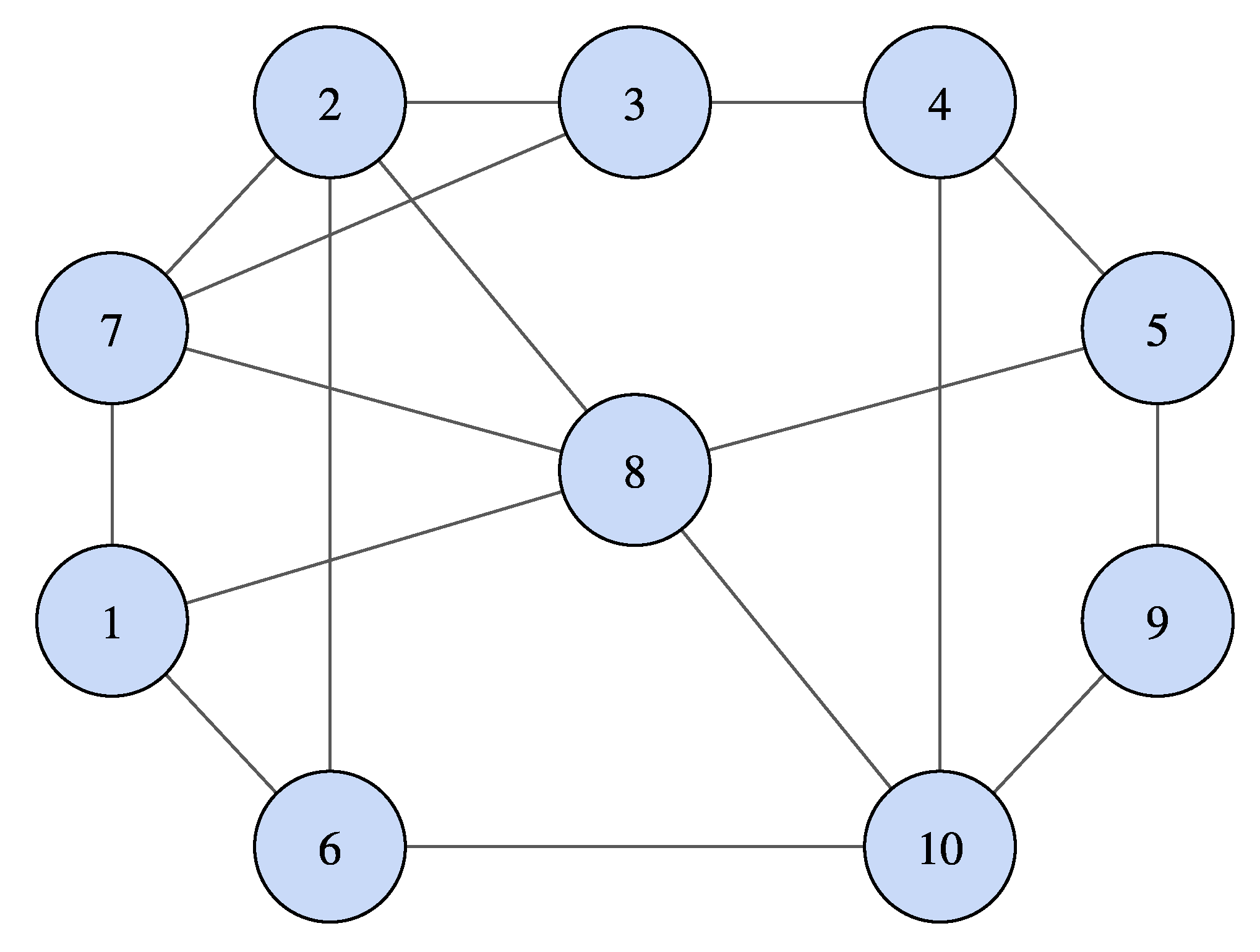
To validate our proposal, we show experiments on a simulation scenario. The communication network for the $\mathsf{N}=10$ agents is described by the graph $\mathcal{G}$ shown in Figure 2. As an example, we consider $m=3$. For this case, we set the gains ${\left\{g_{\mu }\right\}}_{\mu =0}^m=\{48,200,280,160\}$ for all agents, which were chosen as established in Remark 4. We have arbitrarily chosen initial conditions as ${\left\{{\mathsf{\chi }}_{i,0}\left[0\right]\right\}}_{i=1}^{\mathsf{N}}-\mathsf{1}=\{7.27,-2.52,1.63,-7.68,-8.86,9.60,-4.30,1.90,9.24\}$ and ${\mathsf{\chi }}_{\mathsf{N},0}\left[0\right]=-{\sum }_{i=1}^{\mathsf{N}-1}{\mathsf{\chi }}_{i,0}\left[0\right]$ as well as ${\mathsf{\chi }}_{i,\mu }\left[0\right]=0,\forall \mu >0$ to ensure ${\sum }_{i=1}^{\mathsf{N}}{\mathsf{\chi }}_{i,\mu }\left[0\right]=0,\forall \mu \in \{0,\cdots ,m\}$. The internal reference signals for each agent have been provided as $z_i\left(t\right)=A_i\cos ({\omega }_{i}t+{\varphi }_i)$. For the sake of generality, we have arbitrarily chosen the following amplitudes $A_i$, frequencies ${\omega }_i$, and phases ${\varphi }_i$, respectively:

$$\begin{array}{cc}\hfill {\left\{A_i\right\}}_{i=1}^{\mathsf{N}}& =\{33.61,21.58,34.72,12.84,0.49,26.61,13.97,47.31,45.32,19.63\}\hfill \\ \hfill {\left\{{\omega }_i\right\}}_{i=1}^{\mathsf{N}}& =\{1.52,1.15,1.50,1.29,0.25,1.01,0.69,0.18,0.30,0.40\}\hfill \\ \hfill {\left\{{\varphi }_i\right\}}_{i=1}^{\mathsf{N}}& =\{0.02,0.67,0.84,0.97,0.06,0.45,0.58,0.69,0.72,0.65\}\hfill \end{array}$$

(16)

Our goal is to show that we can achieve consistently exact dynamic consensus on the average of the reference signals, $\overline{z}\left(t\right)$, as defined in Remark 1. For our protocol, the error due to the discretization and event-triggered communication is in an arbitrarily small neighbourhood of zero. The desired neighbourhood can be tuned with $\Delta$ and $\epsilon$, according to Theorem 1. Thus, we have tested our proposal with different sampling times $\Delta$ and event thresholds $\epsilon$.

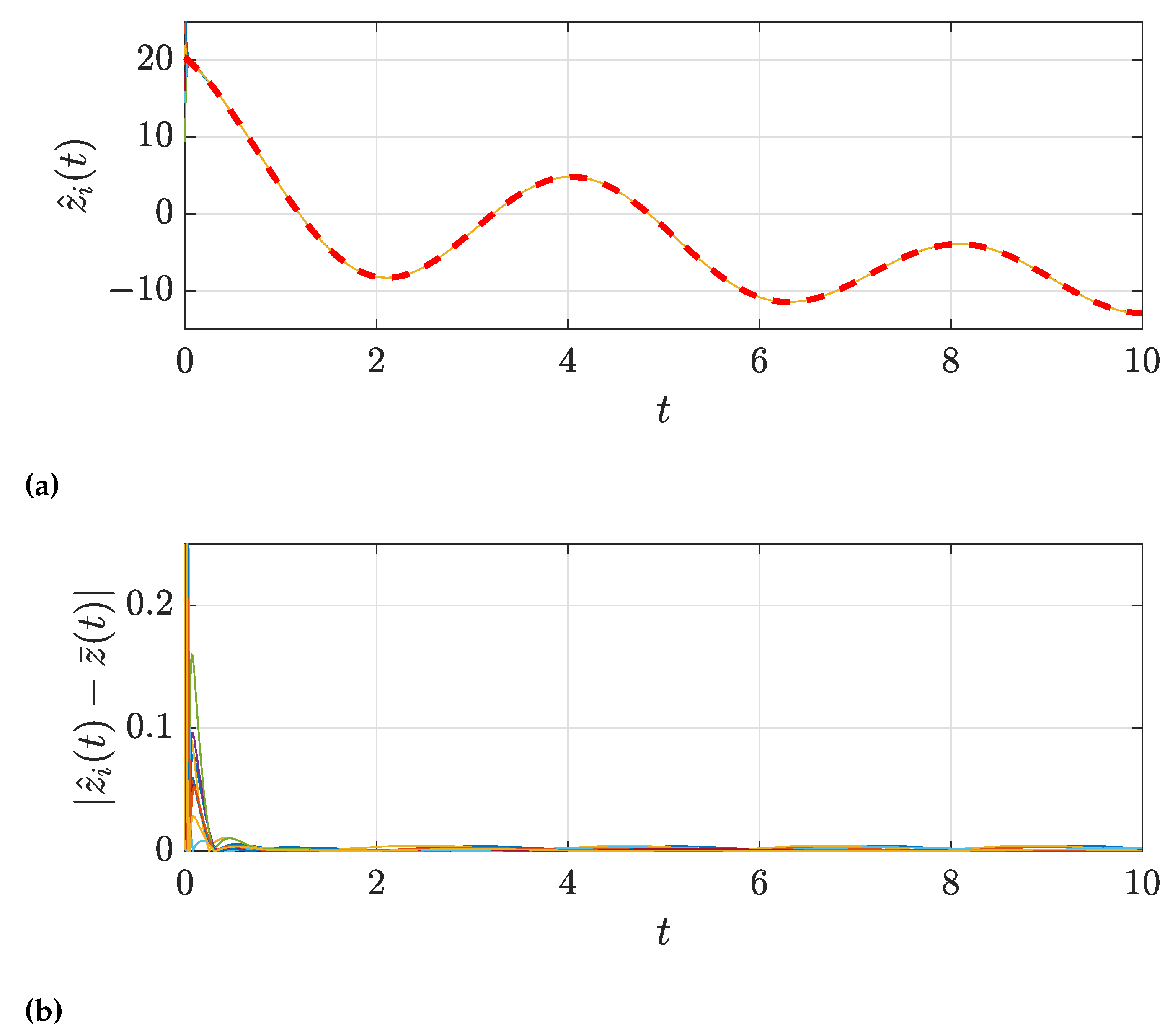
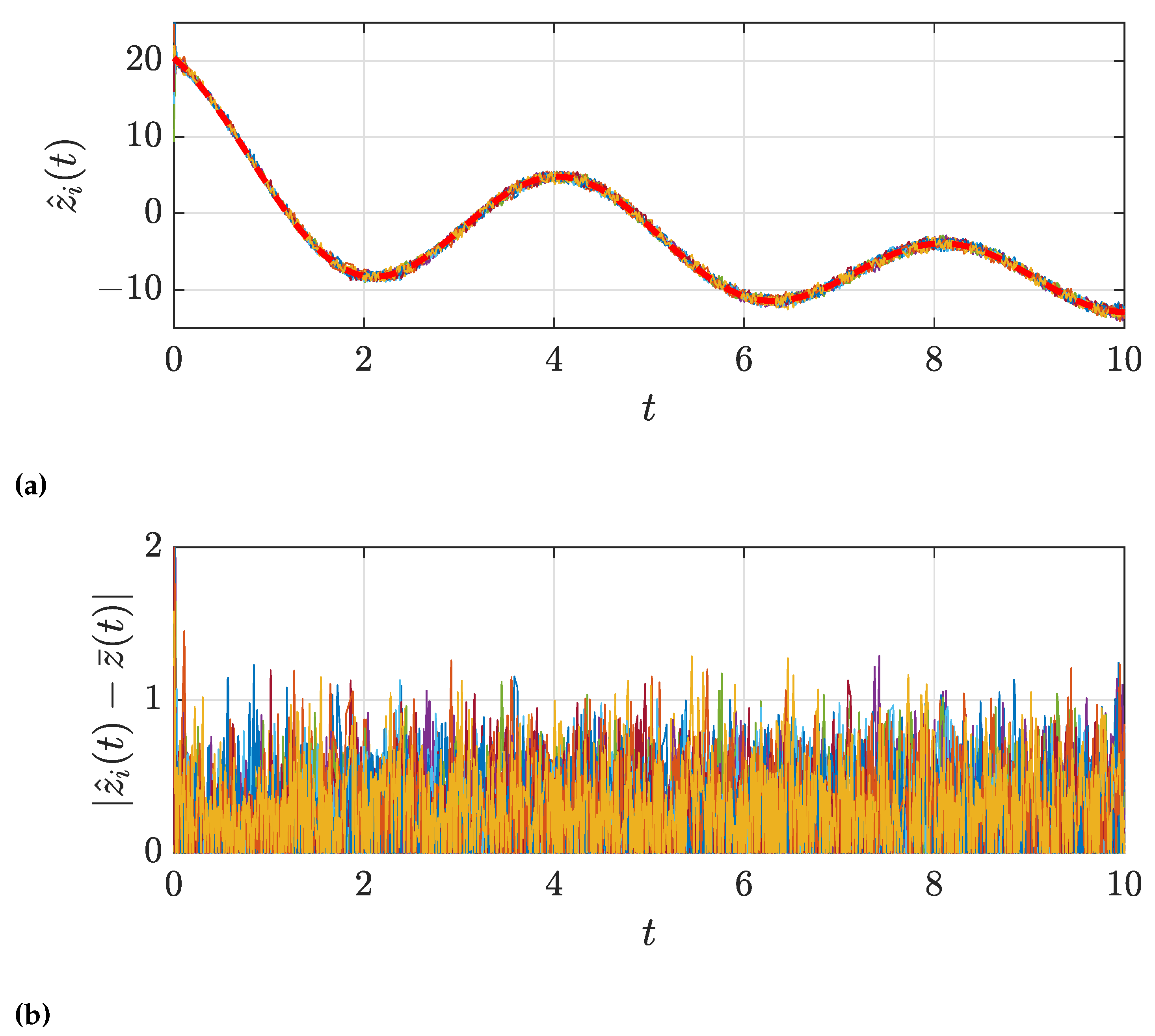
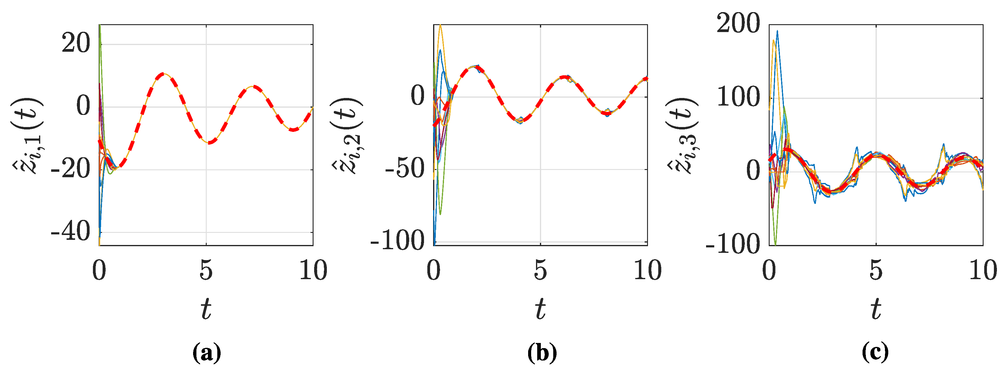
Figure 3 shows the consensus results for our protocol with a sampling period of $\Delta ={10}^{-4}$ and no event-triggered communication ($\epsilon =0)$ as an approximation of the ideal continuous-time case with full communication. For the Figures, we define ${\widehat{z}}_i\left(t\right)={\widehat{z}}_i\left[k\right]$ for $t\in [k\Delta ,(k+1)\Delta )$. The desired dynamic average of the signals, $\overline{z}\left(t\right)$, is plotted in a dashed red line. It can be observed that, after some time, the consensus error falls close to zero.

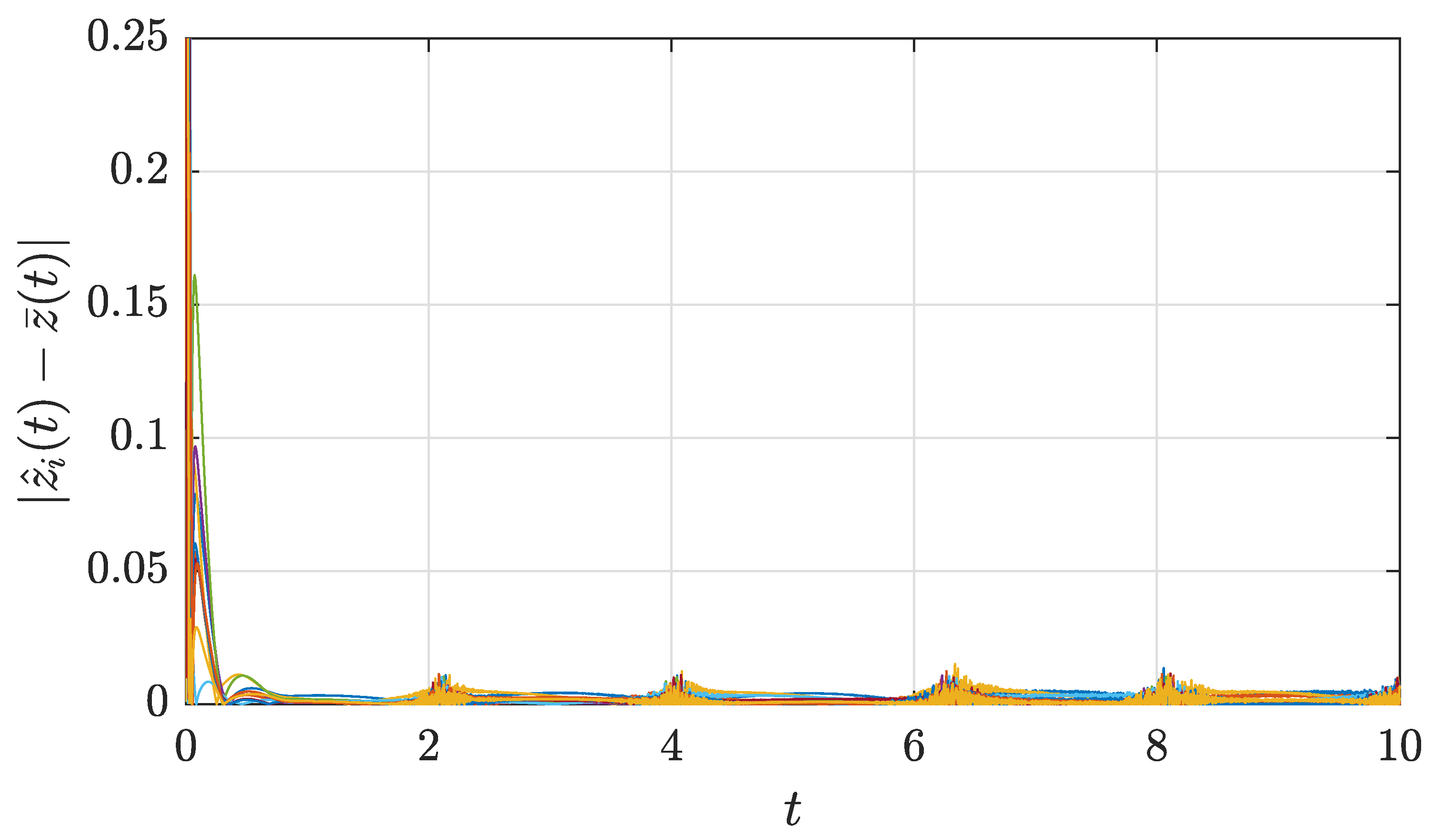
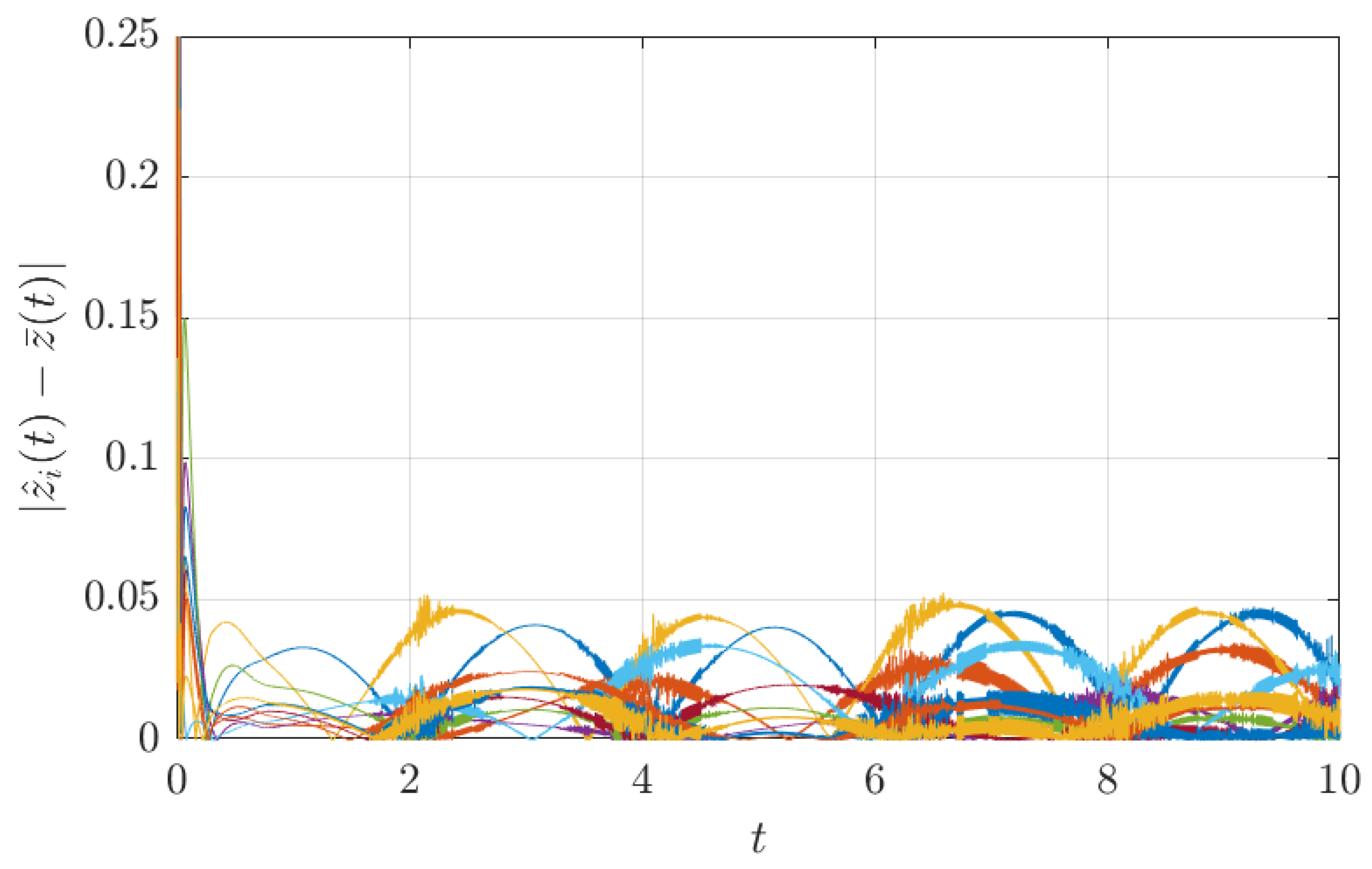
When we add event-triggered communication, the consensus error increases with the value of the triggering threshold $\epsilon$. This can be observed in Figure 4 and Figure 5, which show the results with $\epsilon =0.01$ and $\epsilon =1$, respectively, keeping $\Delta ={10}^{-4}$. Note that, especially for a small $\epsilon$, the event-triggered error is more apparent in the instants where the measured signal changes its slope. This is due to the shape of the event-triggering condition (2), since events are triggered when the current estimate differs from the last transmitted one by more than some threshold $\epsilon$. In the instants around the change in slope, this difference remains smaller than the triggering threshold for a longer time, with the signal around the flat region. Hence, a more noticeable trigger-induced error appears.

The sampling period $\Delta$ also affects the magnitude of the steady-state consensus error. Figure 6 shows the consensus results with $\Delta ={10}^{-3},\epsilon =0.01$. When compared to Figure 4, it is apparent that the consensus error has increased with the sampling period. Note that the oscillating shape of the error is due to the sinusoidal shape of the signal of interest.

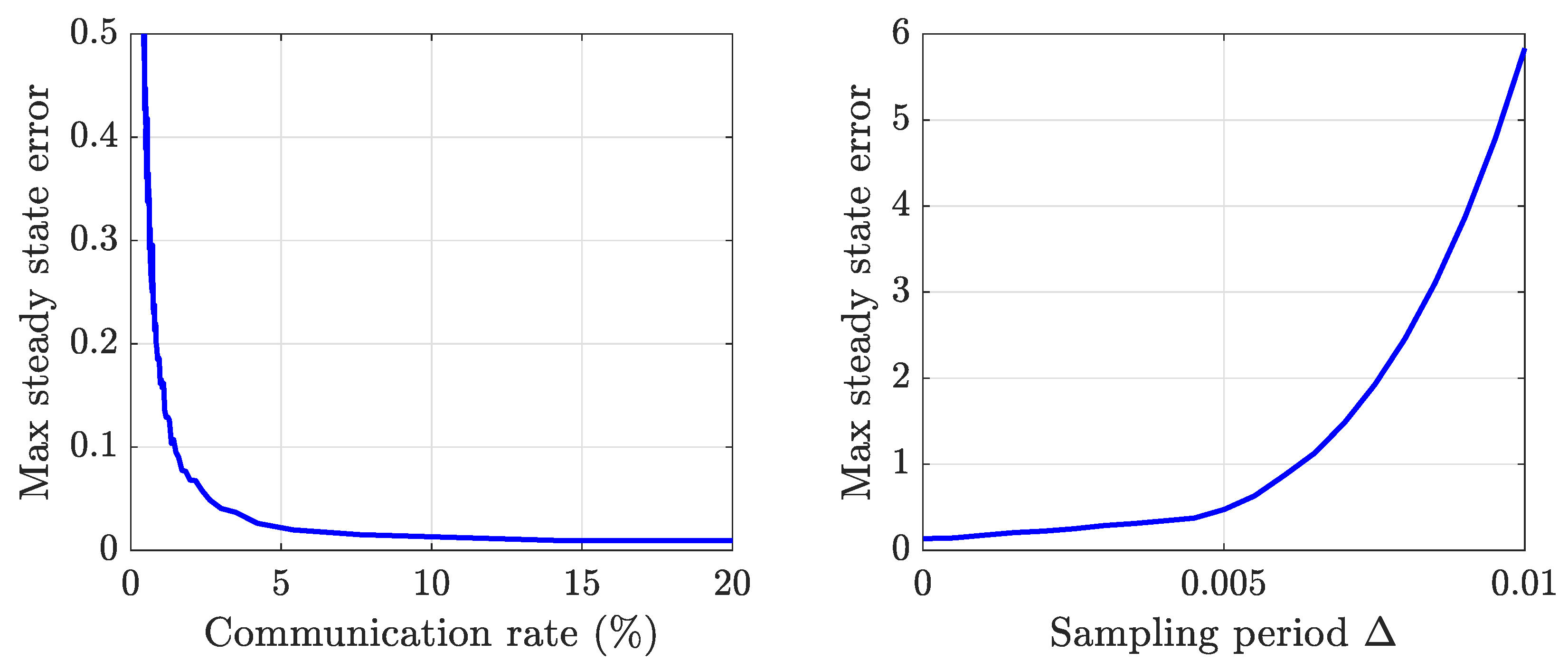
The increase in error due to $\epsilon$ is common in event-triggered setups where there is a trade-off between the number of triggered events and the quality of the results. When we set a higher value of $\epsilon$, we achieve a reduction in communication between agents since information is only exchanged at event instants in the corresponding links, at the cost of an increase in the resulting error. To further analyse the said trade-off, Figure 7 shows the effect that the reduction in communication has on the consensus error. This figure shows that the communication through the network of agents can be significantly reduced with respect to the full communication case without producing a high increase in the steady-state consensus error. The communication rate has been computed as follows:

$$\mathrm{Communication}\mathrm{rate}(\%)=\frac{\mathrm{Messages}\mathrm{sent}\mathrm{between}\mathrm{agents}}{\mathrm{Maximum}\mathrm{possible}\mathrm{messages}}·100$$

(17)

A communication rate of 100% represents full communication, where each agent transmits to all its neighbours at every sampling time. For our proposal, note that when an event is triggered in the link $(i,j)\in \mathcal{E}$, a message is sent from i to its neighbour j and agent j replies with another message to agent i. Thus, for every event that is triggered, two messages are sent through the network. We have considered that when events are triggered in the links $(i,j)$ and $(j,i)$ simultaneously, only one message is sent in each direction.

A similar trade-off is found for the sampling time. Figure 7 also shows the evolution of the consensus error with different values of the sampling period. Note that, if event-triggered communication is used ($\epsilon >0$), the value of $\epsilon$ has a higher impact on the steady-state error than the sampling period when $\Delta \to 0$. In that case, the steady-state error does not asymptotically tend to zero but rather remains in a neighbourhood of zero that is bounded according to $\epsilon$.

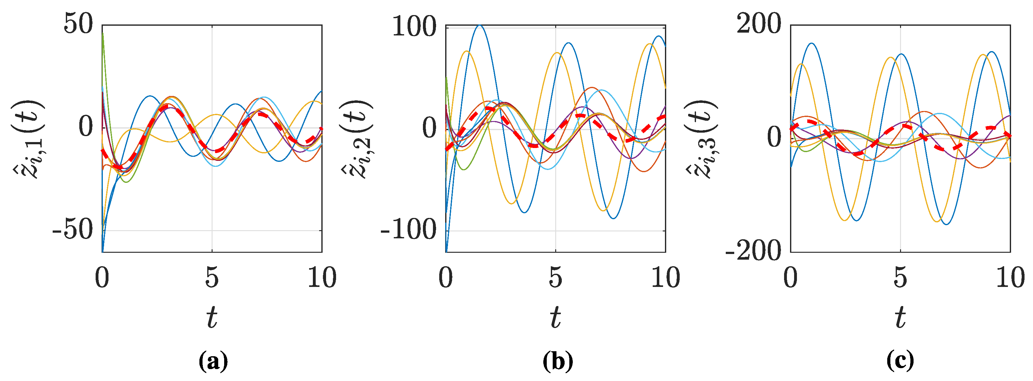
To compare with the other approaches in the literature, we have obtained consensus results for the same simulation scenario using a linear protocol and a First-Order Sliding Modes (FOSM) protocol, which are two existing options for dynamic consensus in the state of the art as described in the following. Note that by performing some adaptations, the linear and FOSM protocols can be obtained as particular cases of our protocol. To implement the linear protocol, we use (3) with $F_{\mu }(•)=(•)$, which is a similar setting as in [4,9]. For the FOSM protocol, we use the equations in (3) setting $m=0$, which correspond to one of the proposals in [20]. For both cases, we set $\Delta ={10}^{-4}$ and $\epsilon =0$ to simulate the case with full communication.

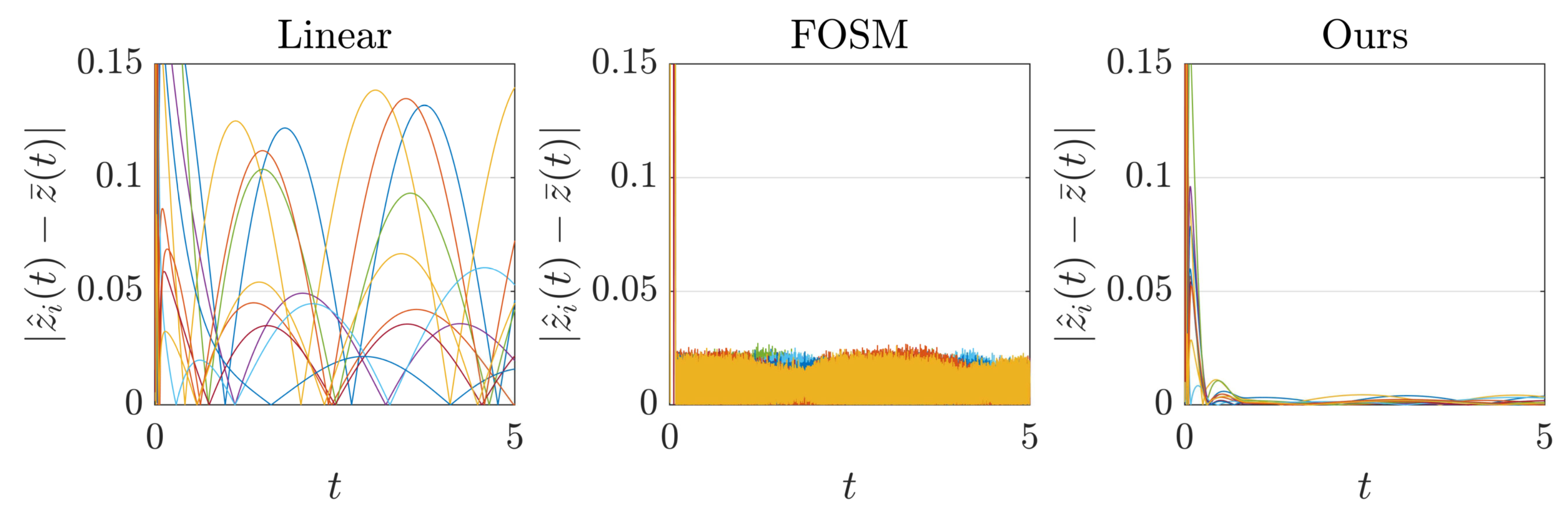
Figure 8 compares the consensus error for the linear and FOSM protocols against our proposal. The FOSM protocol can eliminate the steady-state consensus error in continuous time implementations, but the discretized version suffers from chattering. In contrast, we can see that our method reduces chattering, improving the steady-state error. The linear approach cannot eliminate the permanent consensus error in the estimates of the dynamic average $\overline{z}\left(t\right)$, regardless of the value of $\Delta$ (note that the shape of the error is due to the sinusoidal nature of the signals used in the experiment).

We show the numerical results in

Table 1. Comparison of numerical results for different protocols. Our proposal reduces the estimation error with respect to linear and FOSM protocols in the full communication case. Moreover, adding event-triggered communication to our proposal produces a significant reduction in communication, while still achieving better error values than other protocols.

	Linear [4,9]	FOSM [20]	Ours
			$\epsilon$$=\mathbf{0}$	$\epsilon$$=\mathbf{0}.\mathbf{01}$
Maximum steady state error	0.144	0.027	0.005	0.015
Communication rate	100%	100%	100%	7.61%

to summarize our comparison. We include the maximum steady-state error obtained for the linear and FOSM protocols and for our method. We include the results with full communication ($\epsilon =0$) for comparison and the values obtained with our event-triggered setup ($\epsilon =0.01$). To highlight the advantage of event-triggered communication, we include the level of communication in the network of each approach. The results from Table 1 show that our proposal can significantly reduce the steady-state error compared to the linear and FOSM protocols. Moreover, including event-triggered communication instead of having each agent transmit to all neighbours at every sampling instant produces a drastic reduction in the amount of communication through the network while still performing better than the linear and FOSM protocols with full communication.

Finally, we showed in Corollary 1 that our proposal could also recover the derivatives of the signal of interest with some bounded error. We compare the results obtained for the derivatives against those of a linear protocol. For the FOSM protocol, recall that $m=0$ is used in (3) to compute it and, therefore, it only obtains the internal state ${\mathsf{\chi }}_{i,0}\left[k\right]$, but not the corresponding internal states for the derivatives. Although the linear approach can recover the derivatives of the desired average signal, our proposal is more accurate, as shown in Figure 9 and Figure 10. With our protocol, the derivatives are recovered with some bounded error due to the sampling and event-triggered communication. It can be seen in Figure 10 that this error is more apparent in high-order derivatives and its magnitude can be tuned according to the parameters $\Delta ,\epsilon$, as shown in Corollary 1. Hence, the improvement obtained with our protocol with respect to the linear one is also evident.

5. Comparison to Related Work

In this Section, we offer a qualitative comparison of our work with other methods in the literature. Note that our work is related to the EDCHO protocol presented in [22], which provides a continuous-time formulation of an exact dynamic consensus algorithm. Both works are similar in that they use HOSM to achieve exact convergence. However, since discrete communication is used in practice, our work contributes a discrete-time formulation that guarantees exact convergence when the sampling step approaches zero. Moreover, we have included event-triggered communication to alleviate the communication load in the network of agents.

Other exact dynamic consensus approaches appear in [20,21], which use FOSM. In the discrete-time consensus problem, FOSM protocols suffer from chattering, a steady-state error caused by discretization. The chattering deteriorates the performance of the consensus algorithm in an order of magnitude proportional to the sampling step $\Delta$ when using FOSM. Using HOSM, we have shown in Theorem 1 that our protocol diminishes the effect of chattering. In particular, the error bound is proportional to ${\Delta }^{m+1}$, with m being the order of the sliding modes. We showcased this improvement in the experiment results from Figure 8 and Table 1 in Section 4.

Even though the use of sliding modes results in the exact convergence of the consensus algorithm in continuous-time implementations, several works still rely on linear protocols. A high-order, discrete-time implementation of linear dynamic consensus protocols appears in [9] whose performance does not depend on the sampling step, contrary to our work. Nonetheless, this approach requires the agents to communicate on each sampling instant. This feature is improved in our approach by the use of event-triggered communication.

Many recent works featuring event-triggered schemes to reduce communication among the agents [13,15,29] attain a similar trade-off between the consensus quality and communication rate. However, they also rely on linear consensus protocols. When persistently varying signals are used, this always results in a non-zero steady-state error, which cannot be eliminated even in continuous-time implementations. Hence, even though our event-triggering mechanism is similar to those from other works, our HOSM approach can achieve a vanishing error when $\Delta ,\epsilon$ are arbitrarily small.

6. Conclusions

We have proposed a dynamic consensus algorithm to estimate the dynamic average of a set of time-varying signals in a distributed fashion. By construction, discrete sampling and event-triggered communication are used to reduce the communication burden. The algorithm uses High-Order Sliding Modes, resulting in exact convergence when continuous communication and sampling are used. We have shown that reduced chattering is obtained in the discrete-time setting compared to the First-Order Sliding Modes approach. We have also shown the advantage of our proposal against linear protocols because our protocol can recover the average signal’s derivatives. Finally, we have highlighted the important communication savings that can be achieved by using event-triggered communication between the network agents while maintaining a good trade-off between error and communication. A formal convergence analysis and multiple numerical examples are provided, which verify the proposal’s advantages. We consider removing the constraint on the initial conditions for future work, which will cause the proposal to be robust to the connection or disconnection of agents from the network.

References

1. Aldana-Lopez, R.; Gomez-Gutierrez, D.; Aragues, R.; Sagues, C. Dynamic Consensus with Prescribed Convergence Time for Multileader Formation Tracking. IEEE Control Syst. Lett. 2022, 6, 3014–3019. [Google Scholar] [CrossRef]
2. Chen, F.; Ren, W. A Connection Between Dynamic Region-Following Formation Control and Distributed Average Tracking. IEEE Trans. Cybern. 2018, 48, 1760–1772. [Google Scholar] [CrossRef] [PubMed]
3. Ren, W.; Beard, R.W.; Atkins, E.M. A survey of consensus problems in multi-agent coordination. In Proceedings of the American Control Conference, Portland, OR, USA, 8–10 June 2005; Volume 3, pp. 1859–1864. [Google Scholar]
4. Kia, S.S.; Van Scoy, B.; Cortes, J.; Freeman, R.A.; Lynch, K.M.; Martinez, S. Tutorial on Dynamic Average Consensus: The Problem, Its Applications, and the Algorithms. IEEE Control Syst. Mag. 2019, 39, 40–72. [Google Scholar] [CrossRef] [Green Version]
5. Sen, A.; Sahoo, S.R.; Kothari, M. Distributed Average Tracking With Incomplete Measurement Under a Weight-Unbalanced Digraph. IEEE Trans. Autom. Control 2022, 67, 6025–6037. [Google Scholar] [CrossRef]
6. Iqbal, M.; Qu, Z.; Gusrialdi, A. Resilient Dynamic Average-Consensus of Multiagent Systems. IEEE Control Syst. Lett. 2022, 6, 3487–3492. [Google Scholar] [CrossRef]
7. Peterson, J.D.; Yucelen, T.; Sarangapani, J.; Pasiliao, E.L. Active-Passive Dynamic Consensus Filters with Reduced Information Exchange and Time-Varying Agent Roles. IEEE Trans. Control Syst. Technol. 2020, 28, 844–856. [Google Scholar] [CrossRef]
8. Zhu, M.; Martínez, S. Discrete-time dynamic average consensus. Automatica 2010, 46, 322–329. [Google Scholar] [CrossRef]
9. Montijano, E.; Montijano, J.I.; Sagüés, C.; Martínez, S. Robust discrete time dynamic average consensus. Automatica 2014, 50, 3131–3138. [Google Scholar] [CrossRef]
10. Kia, S.S.; Cortés, J.; Martínez, S. Distributed convex optimization via continuous-time coordination algorithms with discrete-time communication. Automatica 2015, 55, 254–264. [Google Scholar] [CrossRef] [Green Version]
11. Kia, S.S.; Cortés, J.; Martínez, S. Distributed Event-Triggered Communication for Dynamic Average Consensus in Networked Systems. Automatica 2015, 59, 112–119. [Google Scholar] [CrossRef]
12. Zhao, Y.; Xian, C.; Wen, G.; Huang, P.; Ren, W. Design of Distributed Event-Triggered Average Tracking Algorithms for Homogeneous and Heterogeneous Multiagent Systems. IEEE Trans. Autom. Control 2022, 67, 1269–1284. [Google Scholar] [CrossRef]
13. Battistelli, G.; Chisci, L.; Selvi, D. A distributed Kalman filter with event-triggered communication and guaranteed stability. Automatica 2018, 93, 75–82. [Google Scholar] [CrossRef]
14. Yu, D.; Xia, Y.; Li, L.; Zhai, D.H. Event-triggered distributed state estimation over wireless sensor networks. Automatica 2020, 118, 109039. [Google Scholar] [CrossRef]
15. Rezaei, H.; Ghorbani, M. Event-triggered resilient distributed extended Kalman filter with consensus on estimation. Int. J. Robust Nonlinear Control 2022, 32, 1303–1315. [Google Scholar] [CrossRef]
16. Ge, X.; Han, Q.L.; Wang, Z. A dynamic event-triggered transmission scheme for distributed set-membership estimation over wireless sensor networks. IEEE Trans. Cybern. 2019, 49, 171–183. [Google Scholar] [CrossRef] [PubMed]
17. Wu, J.; Jia, Q.S.; Johansson, K.H.; Shi, L. Event-based sensor data scheduling: Trade-off between communication rate and estimation quality. IEEE Trans. Autom. Control 2013, 58, 1041–1046. [Google Scholar] [CrossRef] [Green Version]
18. Peng, C.; Li, F. A survey on recent advances in event-triggered communication and control. Inf. Sci. 2018, 457–458, 113–125. [Google Scholar] [CrossRef]
19. Vasiljevic, L.K.; Khalil, H.K. Error bounds in differentiation of noisy signals by high-gain observers. Syst. Control. Lett. 2008, 57, 856–862. [Google Scholar] [CrossRef]
20. George, J.; Freeman, R.A. Robust Dynamic Average Consensus Algorithms. IEEE Trans. Autom. Control 2019, 64, 4615–4622. [Google Scholar] [CrossRef]
21. Ren, W.; Al-Saggaf, U.M. Distributed Kalman–Bucy Filter With Embedded Dynamic Averaging Algorithm. IEEE Syst. J. 2018, 12, 1722–1730. [Google Scholar] [CrossRef]
22. Aldana-López, R.; Aragüés, R.; Sagüés, C. EDCHO: High order exact dynamic consensus. Automatica 2021, 131, 109750. [Google Scholar] [CrossRef]
23. Aldana-López, R.; Aragüés, R.; Sagüés, C. REDCHO: Robust Exact Dynamic Consensus of High Order. Automatica 2022, 141, 110320. [Google Scholar] [CrossRef]
24. Perruquetti, W.; Barbot, J.P. Sliding Mode Control in Engineering; Marcel Dekker, Inc.: New York, NY, USA, 2002. [Google Scholar]
25. Godsil, C.; Royle, G. Algebraic Graph Theory; Graduate Texts in Mathematics; Springer: Berlin/Heidelberg, Germany, 2001; Volume 207. [Google Scholar]
26. Levant, A. Higher-order sliding modes, differentiation and output-feedback control. Int. J. Control 2003, 76, 924–941. [Google Scholar] [CrossRef]
27. Levant, A. Homogeneity approach to high-order sliding mode design. Automatica 2005, 41, 823–830. [Google Scholar] [CrossRef]
28. Filippov, A.F. Differential equations with discontinuous righthand sides; Mathematics and its Applications (Soviet Series); Kluwer Academic Publishers Group: Dordrecht, The Netherlands, 1988; Volume 18, p. x+304, Translated from the Russian. [Google Scholar]
29. Tan, X.; Cao, J.; Li, X. Consensus of Leader-Following Multiagent Systems: A Distributed Event-Triggered Impulsive Control Strategy. IEEE Trans. Cybern. 2019, 49, 792–801. [Google Scholar] [CrossRef]
30. Rudin, W. Principles of Mathematical Analysis, 3rd ed.; McGraw-Hill Book Company, Inc.: New York, NY, USA; Toronto, ON, Canada; London, UK, 1976. [Google Scholar]
Figure 1. Block diagram for each agent i V . The internal states that the agent computes are updated using the last transmitted estimates of the agent and its neighbours j N i , which are denoted by z ^ i [ k i j ] and z ^ j [ k i j ] , respectively. The current estimate z ^ i [ k ] is computed using the internal state χ i , 0 [ k ] and the local signal z i [ k ] . This estimate is evaluated by the event trigger, which decides if the current value should be transmitted to the neighbours.
Machines 11 00128 g001
Figure 2. Graph G describing the communication network of the N = 10 agents.
Machines 11 00128 g002
Figure 3. Consensus results for our protocol with Δ = 10 4 , ε = 0 (full communication). By using a small time step and communication at every step, our protocol obtains highly precise results. (a) Consensus estimates for the average signal using our proposal. The desired value z ¯ ( t ) is plotted as a dashed red line. The estimates quickly converge to the average signal. (b) Consensus error of the estimates with respect to the average signal. The error converges to a neighbourhood of zero, which can be made arbitrarily small by tuning the value of the sampling period.
Machines 11 00128 g003
Figure 4. Consensus error for our protocol with Δ = 10 4 , ε = 0.01 . The addition of event-triggered communication increases the steady-state consensus error with respect to the full communication case (see Figure 3) and can be tuned with ε .
Machines 11 00128 g004
Figure 5. Consensus results for our protocol with Δ = 10 4 , ε = 1 . Due to the increase in the event-triggering threshold, the error is higher than in the case with ε = 0.01 , shown in Figure 4. (a) Consensus estimates for the average signal using our proposal. The desired value z ¯ ( t ) is plotted as a dashed red line. The estimates quickly converge to the average signal, but with an increased steady-state error due to the event-triggered communication. (b) Consensus error of the estimates with respect to the average signal. Increasing the event-triggering threshold ε causes a higher steady-state error.
Machines 11 00128 g005
Figure 6. Consensus error for our protocol with Δ = 10 3 , ε = 0.01 . Compared to the case shown in Figure 4, with Δ = 10 4 , the consensus error has increased.
Machines 11 00128 g006
Figure 7. Trade-off between the consensus error and the communication rate (with fixed Δ = 10 4 ) and trade-off with the sampling period (with fixed ε = 0.01 ) . As the value of the triggering threshold ε increases, the communication through the network is reduced, at the cost of a higher consensus error. However, using the event-triggering mechanism, communication can be significantly reduced with respect to the full communication case (communication rate of 100%), with a relatively small increase in the steady-state error. The consensus error also increases with the sampling period Δ . When Δ 0 , the parameter ε has a higher impact than Δ on the magnitude of the steady-state error.
Machines 11 00128 g007
Figure 8. Comparison of consensus error with linear protocol, FOSM, and our protocol, under full communication ( Δ = 10 4 , ε = 0 ). With the linear protocol, there exists a permanent steady-state error, which is higher than for the other protocols. Both the FOSM and our protocol can eliminate the error in a continuous-time implementation, but in the discretized setup our method improves the error caused by chattering with respect to the FOSM protocol.
Machines 11 00128 g008
Figure 9. Consensus results for the linear protocol with Δ = 10 4 , ε = 0 , showing the estimates of the derivatives of first (a), second (b), and third (c) order. The derivatives z ¯ ( 1 ) ( t ) , z ¯ ( 2 ) ( t ) , z ¯ ( 3 ) ( t ) are plotted as a dashed red line. High-order derivatives are not accurately computed using a linear protocol.
Machines 11 00128 g009
Figure 10. Consensus results for our protocol with Δ = 10 4 , ε = 0.001 , showing the estimates of the derivatives of first (a), second (b), and third (c) order. The derivatives z ¯ ( 1 ) ( t ) , z ¯ ( 2 ) ( t ) , z ¯ ( 3 ) ( t ) are plotted as a dashed red line. The error induced by the discretization and event-triggered communication is more apparent in higher-order derivatives, but the estimates are greatly improved with respect to the linear protocol (compare to Figure 9).
Machines 11 00128 g010