Narrow Tilting Vehicle Drifting Robust Control

Abstract

The narrow tilting vehicle receives extensive public attention because of traffic congestion and environmental pollution, and the active rolling motion control is a traffic safety precaution that reduces the rollover risk caused by the structure size of the narrow vehicle. The drifting motion control reflects the relatively updated attentive research of the regular-size vehicle, which can take full advantage of the vehicle’s dynamic performance and improve driving safety, especially when tires reach their limits. The narrow tilting vehicle drifting control is worthy of research to improve the driving safety of the narrow tilting vehicle, especially when tires reach the limit. The nonlinear narrow tilting vehicle dynamic model is established with the UniTire model to describe the vehicle motion characteristics and is simplified to reduce the computation of the drifting controller design. The narrow tilting vehicle drifting controller is designed based on the robust theory with uncertain external disturbances. The controller has a wide application, validity, and robustness and whose performance is verified by realizing different drifting motions with different initial driving motions. The narrow tilting vehicle drifting robust control has some practical and theoretical significance for more research.

1. Introduction

With increasing population and rapid economic development, there are continuing high numbers of vehicle population as [1] and traffic accidents as [2,3]. The mini-size vehicle has been paid close attention to universally, and the narrow tilting vehicle entered the public consciousness. The narrow tilting vehicle is designed to solve traffic congestion and environmental pollution problems caused by the vehicle’s rapid growth. Furthermore, the active rolling motion of the narrow tilting vehicle is the steady state realized by the active rolling controller based on the velocity and the steering angle to avoid the rollover.

Traffic safety is in constant focus [4], and most relative research includes the autonomous steering of the regular-size vehicle [5] and the active rolling of the narrow vehicle. The autonomous steering of regular-size vehicle research is almost wholly working under the linear vehicle and tire condition, such as the path following in [6] and the human-machine cooperation driving in [7]. Most traffic safety research on narrow vehicles has looked at how to reduce the rollover risk. The active rolling of the narrow vehicle can improve turning driving safety and avoid the rollover risk caused by the narrow size. The narrow vehicle is divided into direct tilt control and steering tilt control [8] based on active rolling methods. It is also divided into the four-wheel [9], the three-wheel [10], and the reversed three-wheel [11] based on the structures. The direct tilt control of the narrow tilting vehicle is directly applied to the vehicle body, but it has poor adaptability under different working conditions. The narrow tilting vehicle based on the steering tilting control realizes the active rolling based on the steering angle, but it needs the driving technique and is not well suited at the low longitudinal velocity. The narrow tilting vehicle studied in this paper is a four-wheel narrow tilting vehicle with direct tilt control based on the steering angle [12] to improve driving safety at a multi-level velocity in different steering angles. The active rolling target angle is the steady state calculated based on the centrifugal force balance analysis in [13], which is realized by relying on the active rolling mechanic [12,14]. The narrow tilting vehicle studied in this paper is verified whereby the active rolling angle can realize the steady-state target and lower the rollover risk significantly by the active rolling mechanic and controller [12,13,14]. Most other traffic safety research on the narrow tilting vehicle focuses on vehicle performance under normal working conditions, as seen in one study [15].

The drifting motion control is a unique control strategy available to enhance traffic safety, which is little used in narrow drifting motions. The drifting movement of the racing car can be controlled by the drifting controller, which realizes the target drifting motion analyzed based on the three-of-freedom vehicle dynamics model when tires reach the maximum in [16]. The regular-size vehicle drifting motion parameters, including velocity, sideslip angle, yaw rate, and steering angle can be calculated and obtained by analyzing the steady-state vehicle dynamics expressions in the adhesion limit [17], and the drifting controllers of a regular-size vehicle are designed based on the linear quadratic regulator theory [17,18,19], the model predictive control theory [20,21], and the adaptive control theory [22]. There is reinforcement learning [18], and neural networks [23] are applied to the vehicle drifting control based on existing vehicle drifting motion parameters. Most drifting research without the learning realize the target drifting motion, which is the core work, and ignores some important details which affect the practical implementation, especially disturbances. Most drifting research based on the learning realize the passed path under drifting motions, and the adaptability in different working conditions are not fully verified, and most vehicle dynamics models of drifting movements are very similar to the classic one [24] that suggests vehicle dynamics with no-active rolling. According to the narrow tilting vehicle characteristics, it is necessary to design a drifting controller with extensive suitability with external disturbances to improve driving safety when tires reach the maximum. The robust theory performs better in solving problems caused by disturbances and can accommodate engineering requirements in practice. The linear matrix inequality (LMI) is widely applied in solving the problems of controller and system designs, which has become popular in the controller solution, especially in the robust controller.

From the above analysis, this paper researches how to control the narrow tilting vehicle drifting motions. According to the narrow tilting vehicle characteristics, the non-linear narrow tilting vehicle dynamics model is established to describe the vehicle motion characteristics and is appropriately simplified to reduce the computing effort in the drifting controller design. The narrow tilting vehicle drifting controller is designed based on the robust theory with uncertain extern disturbances considering the practical application environment, which is relatively independent and does not affect the active rolling controller working. The performance of the drifting controller is tested to realize different target drifting motions based on different initial motions, which can express the reliability, availability, and universality of the designed controller.

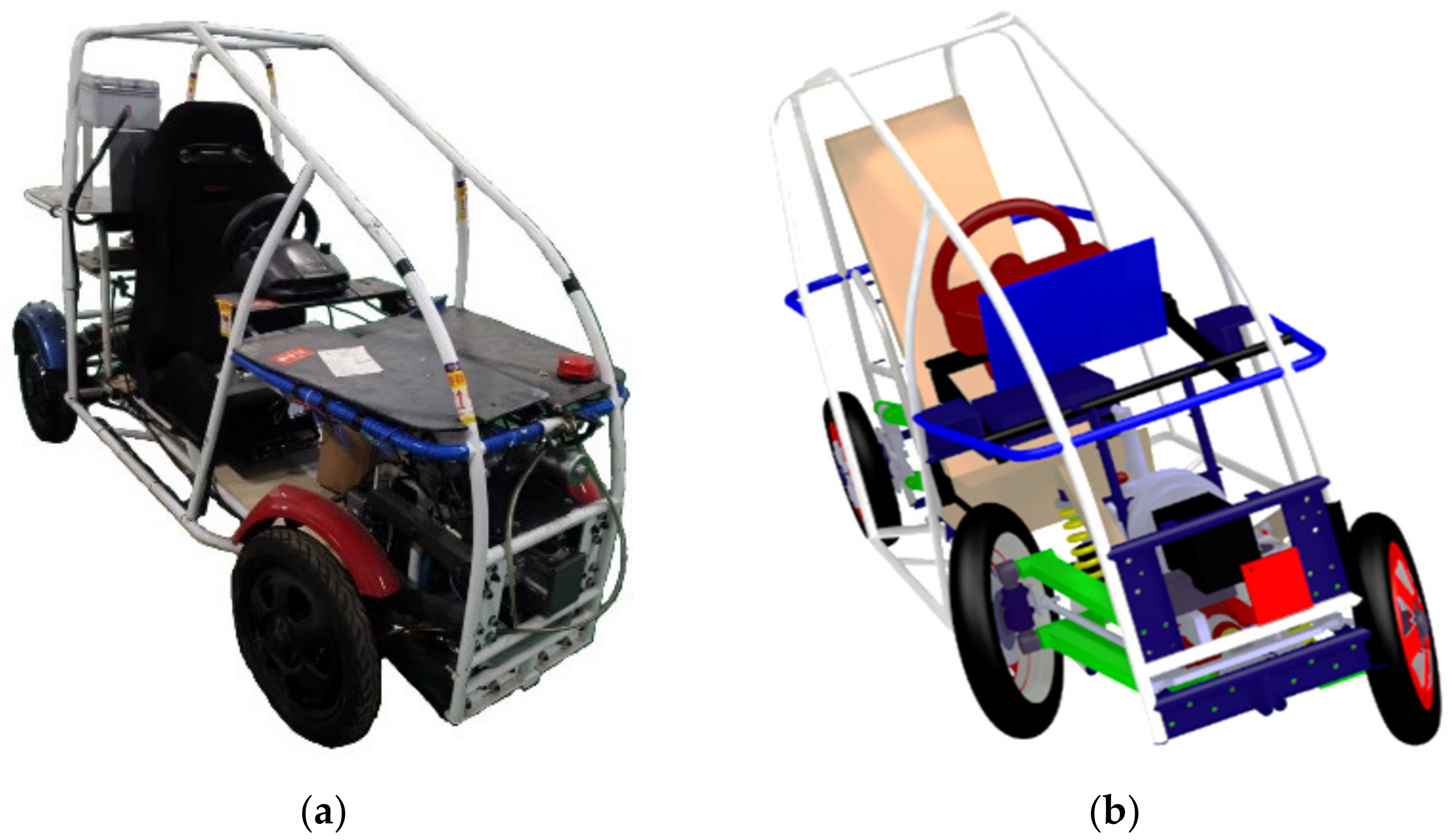
2. Narrow Tilting Vehicle Dynamics System for Drifting Controller Design

The narrow tilting vehicle shown in Figure 1a, whose structural diagram is shown in Figure 1b in [25], avoids rollover danger by the active roll control, which is different from most vehicles. To ensure all wheels are on the ground and avoid rollover, the rolling controller of the narrow tilting vehicle creates a good balance between the gravity component caused by rolling and centrifugal force caused by turning [12,13,14].

The vehicle dynamics system is requested to describe the narrow tilting vehicle drifting motion characteristics and is applied to the controller design to realize target motions. The rolling motion of the narrow tilting vehicle is different from most vehicles; as a result, the major influence factors of the vertical load transfer are distinctive. The drifting motion is a unique motion state for the vehicle, and tire forces reach limits in the drifting motion. Therefore, the tire model also has an essential effect on the controller design.

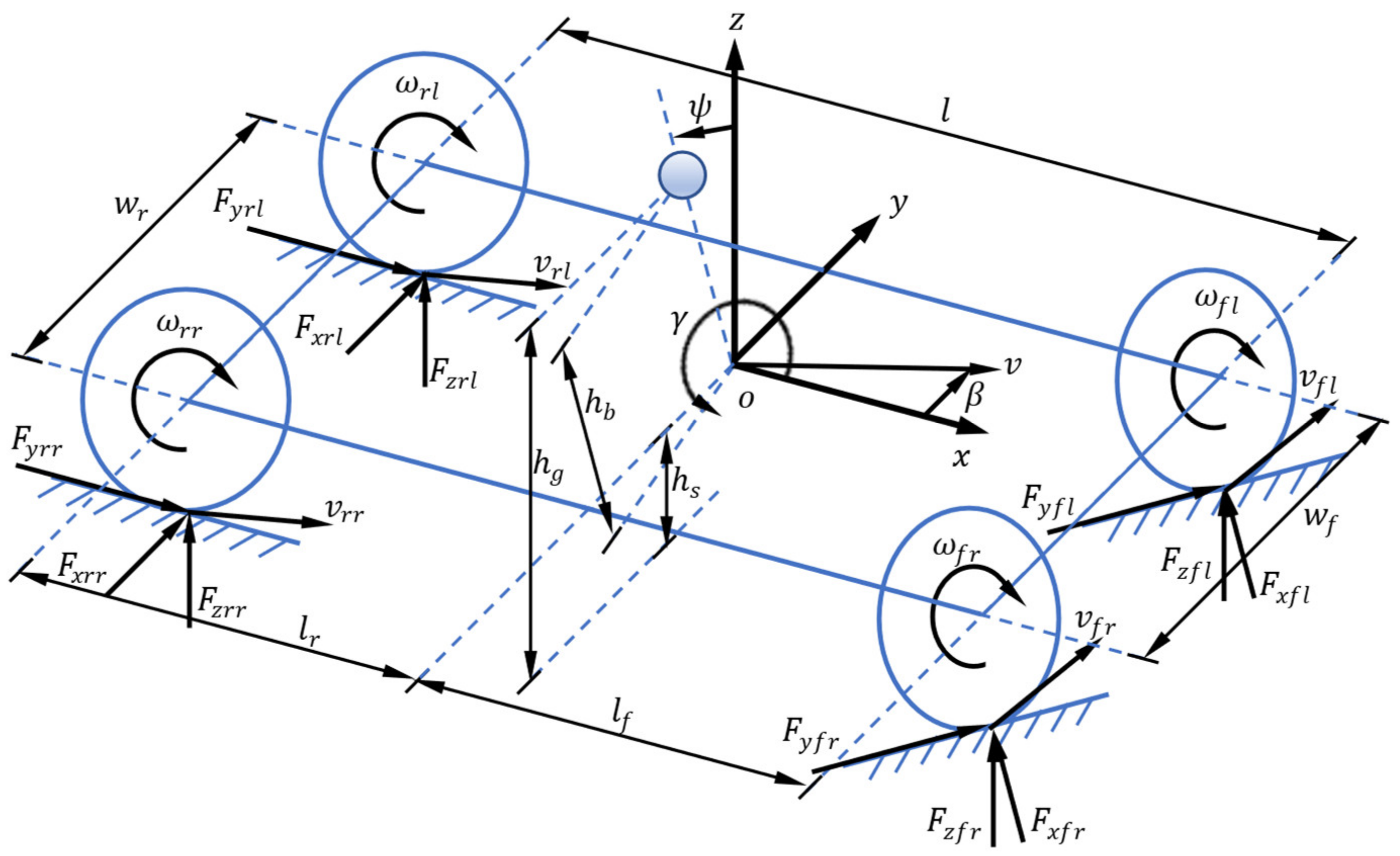
2.1. Narrow Tilting Vehicle Dynamics Equations

The active rolling movement meets the need for the active rolling angle for the centrifugal force equilibrium based on narrow tilting vehicle dynamics characteristics. The vehicle dynamics model, including the active rolling movement, is shown in Figure 2 and is described as Equations (1)–(4), where Equation (5) describes the normal rolling motion without the active rolling mechanic.

$$\begin{array}{ll}\dot{v}& =\left(F_{xfl}+F_{xfr}\right)\left(\frac{\cos {\delta }_f\cos \beta }{m}+\frac{\sin {\delta }_f\sin \beta }{m}\right)+\left(F_{yfl}+F_{yfr}\right)\left(-\frac{\sin {\delta }_f\cos \beta }{m}+\frac{\cos {\delta }_f\sin \beta }{m}\right)\\ & +\left(F_{xrl}+F_{xrr}\right)\frac{\cos \beta }{m}+\left(F_{yrl}+F_{yrr}\right)\frac{\sin \beta }{m}-\frac{C_d{A}_f{v}^2{\cos }^3\beta }{21.15m},\end{array}$$

(1)

$$\begin{array}{ll}\dot{\beta }=& -\gamma +\left(F_{xfl}+F_{xfr}\right)\left(\frac{\sin {\delta }_f\cos \beta }{mv}-\frac{\cos {\delta }_f\sin \beta }{mv}\right)+\left(F_{yfl}+F_{yfr}\right)\left(\frac{\cos {\delta }_f\cos \beta }{mv}+\frac{\sin {\delta }_f\sin \beta }{mv}\right)\\ & -\left(F_{xrl}+F_{xrr}\right)\frac{\sin \beta }{mv}+\left(F_{yrl}+F_{yrr}\right)\frac{\cos \beta }{mv}+\frac{C_d{A}_{f}v{\cos }^2\beta \sin \beta }{21.15m},\end{array}$$

(2)

$$\begin{array}{ll}\dot{\gamma }& =\frac{l_f}{I_z}\left(F_{xfl}+F_{xfr}\right)\sin {\delta }_f+\frac{l_f}{I_z}\left(F_{yfl}+F_{yfr}\right)\cos {\delta }_f-\frac{l_r}{I_z}\left(F_{yrl}+F_{yrr}\right)-\frac{w_f}{2I_z}\left(F_{xfl}-F_{xfr}\right)\cos {\delta }_f\\ & +\frac{w_f}{2I_z}\left(F_{yfl}-F_{yfr}\right)\sin {\delta }_f-\frac{w_r}{2I_z}\left(F_{xrl}-F_{xrr}\right),\end{array}$$

(3)

$$\psi =-{\tan }^{-1}\frac{v^2}{g{R}_r},$$

(4)

$$\ddot{\psi }=\frac{I_{xz}}{I_x}\dot{\gamma }+\frac{m_b{h}_b}{I_x}\left({\dot{v}}_y+v_x\gamma \right)+\frac{m_{b}g{h}_b}{I_x}\sin \psi -\frac{K_{\psi }\psi +C_{\psi }\dot{\psi }}{I_x}$$

(5)

where $m$ is the vehicle mass, $m_b$ is the vehicle body mass, $h_b$ is the height of gravity center from the roll axis, $l_f$ and $l_r$ are the distances from gravity center to front and rear axle, $w_f$ and $w_r$ are the distances between left and right wheels of the front and rear axle, $R_r=\left(l_f+l_r\right)/{\delta }_f$ is the ideal turning radius calculated based on the steering angle, $v$ and $\dot{v}$ are the vehicle velocity and accelerated velocity, $\beta$ and $\dot{\beta }$ are the vehicle sideslip angle and rate, $\gamma$ and $\dot{\gamma }$ are the vehicle yaw rate and angular acceleration, ${\delta }_f$ is the front-wheel steering angle, $\psi$ is the vehicle steady roll angle and is implemented by the active roll controller, $I_z$ is the moment of inertia with respect to yaw axis, $C_d$ is the aerodynamics drag coefficient, $A_f$ is the vehicle frontal area, and $F_{xij}$ and $F_{yij}$ ($i=f,r$; $j=l,r$) are the longitudinal and lateral forces at each tire, respectively, the index $i=f,r$ is used to express the front and rear axles, and the index $j=l,r$ is used to express the left and right wheels.

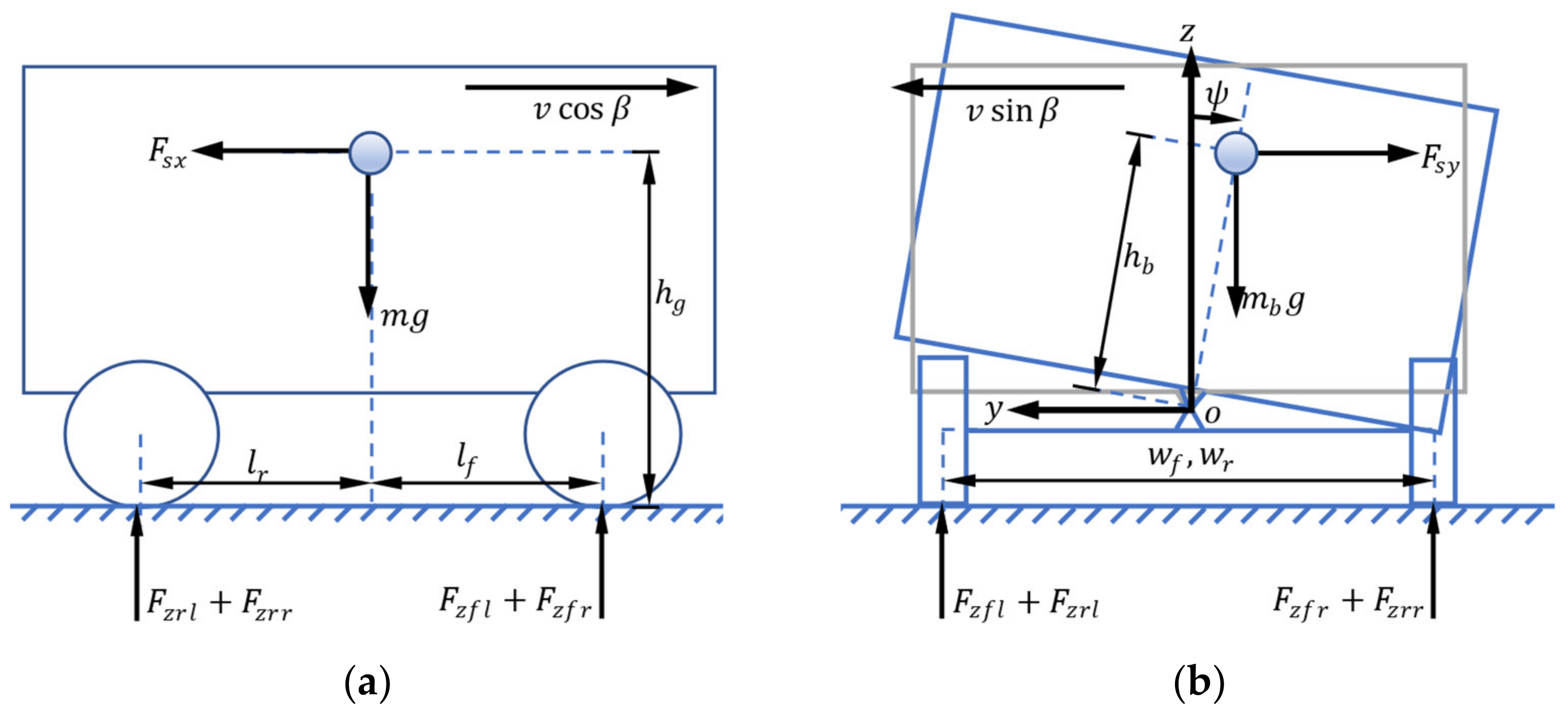
2.2. Vertical Load Transfer

The rolling movement of the narrow tilting vehicle is distinctive. The roll angle has a significant influence on the vertical load transfer. Considering the load transfer caused by longitudinal and lateral forces and the active roll control shown in Figure 3, the vertical force at each tire can be described as Equations (6)–(9).

$$F_{zfl}=\frac{mg{l}_r}{2\left(l_f+l_r\right)}-\frac{F_{sx}{h}_g}{2\left(l_f+l_r\right)}-\frac{l_r\left(F_{sy}{h}_g\cos \psi +m_{b}g{h}_b\sin \psi \right)}{\left(l_f+l_r\right)w_f},$$

(6)

$$F_{zfr}=\frac{mg{l}_r}{2\left(l_f+l_r\right)}-\frac{F_{sx}{h}_g}{2\left(l_f+l_r\right)}+\frac{l_r\left(F_{sy}{h}_g\cos \psi +m_{b}g{h}_b\sin \psi \right)}{\left(l_f+l_r\right)w_f},$$

(7)

$$F_{zrl}=\frac{mg{l}_f}{2\left(l_f+l_r\right)}+\frac{F_{sx}{h}_g}{2\left(l_f+l_r\right)}-\frac{l_f\left(F_{sy}{h}_g\cos \psi +m_{b}g{h}_b\sin \psi \right)}{\left(l_f+l_r\right)w_r},$$

(8)

$$F_{zrr}=\frac{mg{l}_f}{2\left(l_f+l_r\right)}+\frac{F_{sx}{h}_g}{2\left(l_f+l_r\right)}+\frac{l_f\left(F_{sy}{h}_g\cos \psi +m_{b}g{h}_b\sin \psi \right)}{\left(l_f+l_r\right)w_r},$$

(9)

where $h_g$ is the height of gravity center, $F_{sx}=\left(F_{xfl}+F_{xfr}\right)\cos {\delta }_f-\left(F_{yfl}+F_{yfr}\right)\sin {\delta }_{fl}+\left(F_{xrl}+F_{xrr}\right)-C_d{A}_f{v}^2{\cos }^3\beta /\left(21.15m\right)$, and $F_{sy}=\left(F_{xfl}+F_{xfr}\right)\sin {\delta }_{fl}+\left(F_{yfl}+F_{yfr}\right)\cos {\delta }_{fl}+\left(F_{yrl}+F_{yrr}\right)$.

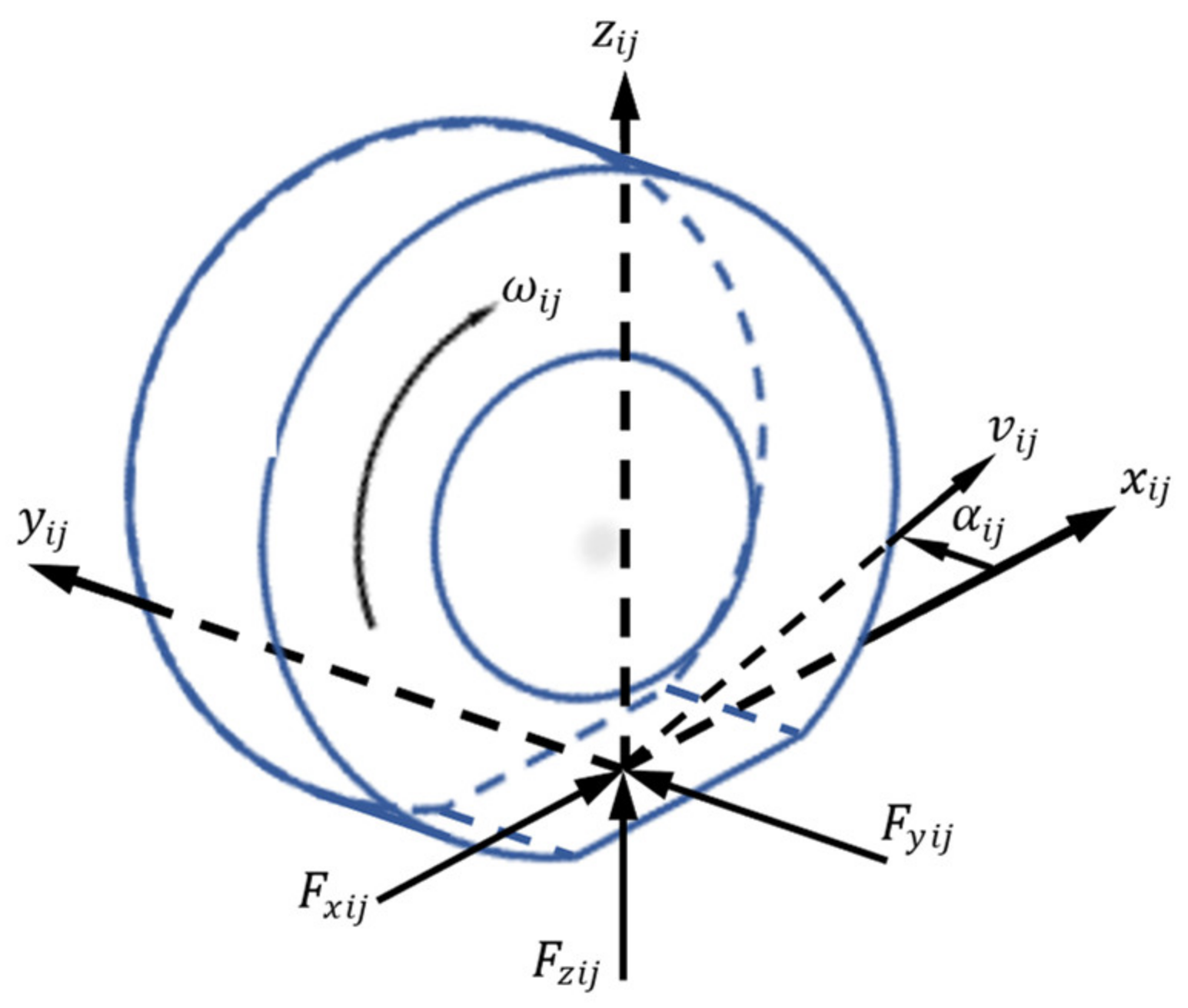
2.3. Tire Models and Equations

The vehicle drifting motion is nonlinear, and tire forces reach the maximum while the steering angle is non-vanishing in the drifting motion. Therefore, the nonlinear tire model is essential in this system to describe the force condition at each tire. The UniTire tire model can express tire forces more accurately not only in single working conditions but also in complex working conditions [26], which means it is ideally suited to the part of the vehicle drifting motion. If the UniTire tire model is applied directly to the narrow tilting vehicle drifting controller, there will be a large amount of computation in the controller design. The linearized tire model based on UniTire is proposed in the controller design to solve this problem and express tire forces accurately. Thus, UniTire describes tire forces during the narrow tilting vehicle motion, and the linearized tire model is applied to the narrow tilting drifting controller design.

2.3.1. UniTire

UniTire can express longitudinal and lateral tire forces and overturning, rolling resistance, and aligning tire moments based on the tire coordinate system and is applicated to the vehicle dynamics simulation and the vehicle motion controller design [27]. In this paper, the tire model is applied to express longitudinal and lateral tire forces, which are the main characteristics of different working conditions. Thus, the simplified tire coordinate system is shown in Figure 4 with the consideration of longitudinal and lateral tire motions and the neglect of tire moments, and the equations of the tire model are described as Equation (10).

$$\left\{\begin{array}{c}{\overline{F}}_{ij}=1-e^{-{\varphi }_{ij}-E{\varphi }_{ij}{}^2-\left(E^2+\frac{1}{12}\right){\varphi }_{ij}{}^3}\\ F_{xij}={\overline{F}}_{ij}\frac{{\varphi }_{xij}}{{\varphi }_{ij}}{\mu }_{xij}{F}_{zij}\\ F_{yij}={\overline{F}}_{ij}\frac{{\varphi }_{yij}}{{\varphi }_{ij}}{\mu }_{yij}{F}_{zij}\end{array}\right.,$$

(10)

where ${\overline{F}}_{ij}$ ($i=f,r$; $j=l,r$) is the normalized force, $E$ is the curvature factor of the combined slip resultant force and is the variable related to the tire slip ratios in [28], ${\mu }_{xij}$ and ${\mu }_{yij}$ ($i=f,r$; $j=l,r$) are the longitudinal and lateral friction coefficient, ${\varphi }_{xij}=K_{xij}{S}_{xij}/\left({\mu }_{xij}{F}_{zij}\right)$, ${\varphi }_{yij}=K_{yij}{S}_{yij}/\left({\mu }_{yij}{F}_{zij}\right)$, and ${\varphi }_{ijj}=\sqrt{{\varphi }_{xij}{}^2+{\varphi }_{yij}{}^2}$ ($i=f,r$; $j=l,r$) are normalized longitudinal, lateral and combined slip ratios, $S_{xij}=\left({\omega }_{ij}{r}_{eij}-v_{ij}\cos {\alpha }_{ij}\right)/\left({\omega }_{ij}{r}_{eij}\right)$ and $S_{yij}=-v_{ij}\sin {\alpha }_{ij}/\left({\omega }_{ij}{r}_{eij}\right)$ ($i=f,r$; $j=l,r$) are the longitudinal and lateral slip ratios in UniTire, $K_{xij}$ and $K_{yij}$ ($i=f,r$; $j=l,r$) are the longitudinal slip and cornering stiffness of the tire based on $S_{xij}$ and $S_{yij}$, $v_{ij}$ ($i=f,r$; $j=l,r$) is the wheel velocity, ${\omega }_{ij}$ ($i=f,r$; $j=l,r$) is the wheel rotation angular velocity, $r_{eij}$ ($i=f,r$; $j=l,r$) is the wheel effective rolling radius, ${\alpha }_{ij}$ ($i=f,r$; $j=l,r$) is the wheel slip angle, and the wheel slip angle of each wheel respectively satisfy ${\alpha }_{fl}={\tan }^{-1}\left(\left(-a_{fl}\sin {\delta }_f+\left(v\sin \beta +l_f\gamma \right)\cos {\delta }_f\right)/\left(a_{fl}\cos {\delta }_f+\left(v\sin \beta +l_f\gamma \right)\sin {\delta }_f\right)\right)$, ${\alpha }_{fr}={\tan }^{-1}\left(\left(-a_{fr}\sin {\delta }_f+\left(v\sin \beta +l_f\gamma \right)\cos {\delta }_f\right)/\left(a_{fr}\cos {\delta }_f+\left(v\sin \beta +l_f\gamma \right)\sin {\delta }_f\right)\right)$, ${\alpha }_{rl}={\tan }^{-1}\left(\left(v\sin \beta -l_r\gamma \right)/\left(v\cos \beta -w_r\gamma /2\right)\right)$, and ${\alpha }_{rr}={\tan }^{-1}\left(\left(v\sin \beta -l_r\gamma \right)/\left(v\cos \beta +w_r\gamma /2\right)\right)$ in which $a_l=v\cos \beta -w_f\gamma /2$ and $a_r=v\cos \beta +w_f\gamma /2$.

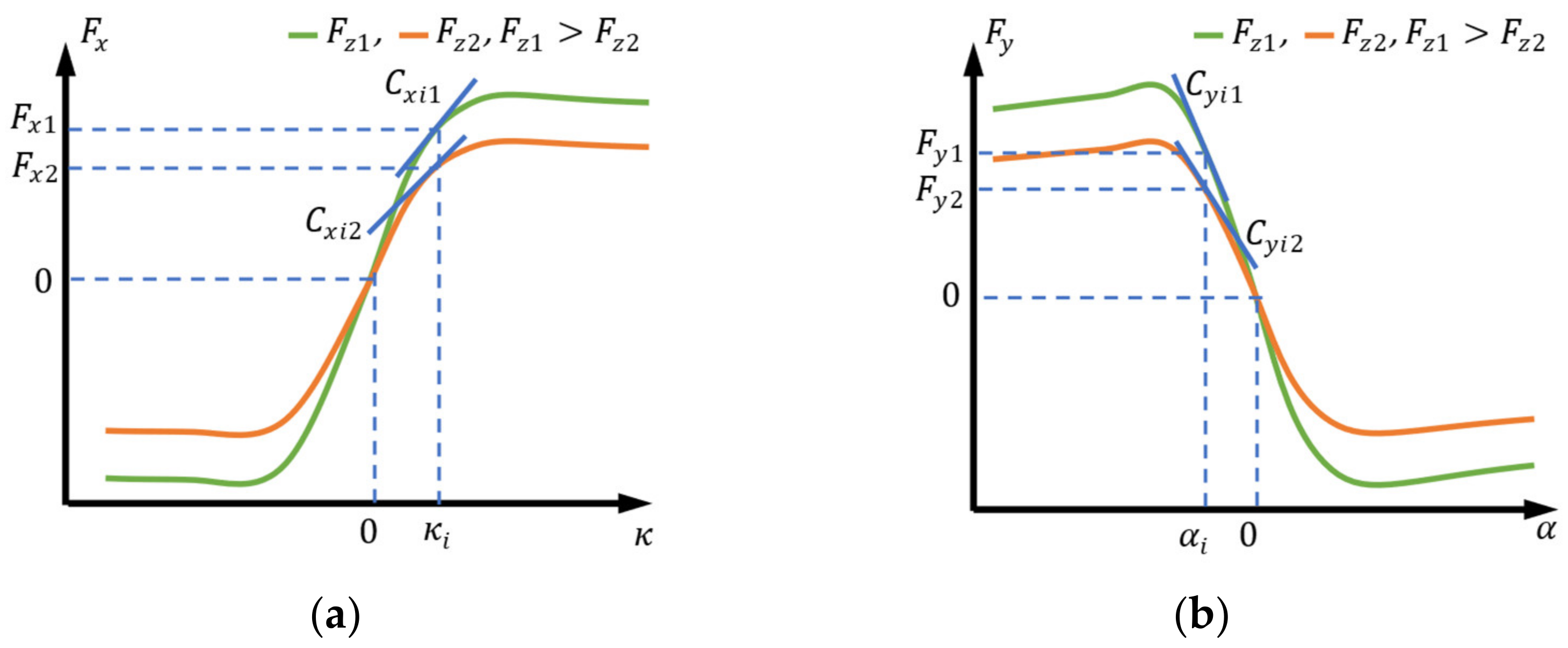
2.3.2. The Linearized Tire Equations

UniTire is a nonlinear tire model, and its tire force equations are complicated for the controller design. The linearized tire equations are derived based on the representation of the nonlinear tire model. The TYDEX longitudinal slip ratio is the common expression, and the nonlinear tire model representation is shown in Figure 5.

According to the UniTire representation, the nonlinear tire model can be approximately linearized and divided into many groups. The slip angles of the left and right wheels in the same axle are less differentiating based on the expression of slip angles, which has a slight influence on tire forces, and it suggests that the value of the vertical force makes a difference to the tire force value, the slip stiffness, and the cornering stiffness in Figure 5. The linearized tire equations are described as Equation (11) with the consideration of the simplified calculation of the controller system and the independent control of the front and rear axles.

$$\left\{\begin{array}{c}{F}_{xij}={\widehat{C}}_{xij}\left({\kappa }_i-{\widehat{\kappa }}_i\right)+{\widehat{F}}_{xij}\\ F_{yij}={\widehat{C}}_{yij}\left({\alpha }_i-{\widehat{\alpha }}_i\right)+{\widehat{F}}_{yij}\end{array}\right.,$$

(11)

where ${\kappa }_i=-\left(v_i\cos {\alpha }_i-{\omega }_i{r}_{ei}\right)/\left(v_i\cos {\alpha }_i\right)$ ($i=f,r$) is the TYDEX longitudinal slip ratio, ${\widehat{\kappa }}_i$, ${\widehat{\alpha }}_i$, ${\widehat{C}}_{xij}$, ${\widehat{C}}_{yij}$, ${\widehat{F}}_{xij}$, and ${\widehat{F}}_{yij}$ are the known slip ratio, slip angle, slip stiffness, cornering stiffness, longitudinal force, and lateral force of the approximation point, respectively, ${\alpha }_f={\tan }^{-1}\left(\left(-v\cos \beta \sin {\delta }_f+\left(v\sin \beta +l_f\gamma \right)\cos {\delta }_f\right)/\left(v\cos \beta \cos {\delta }_f+\left(v\sin \beta +l_f\gamma \right)\sin {\delta }_f\right)\right)$ is the slip angle of the front axle, and ${\alpha }_r={\tan }^{-1}\left(\left(v\sin \beta -l_r\gamma \right)/\left(v\cos \beta \right)\right)$ is the slip angle of the rear axle.

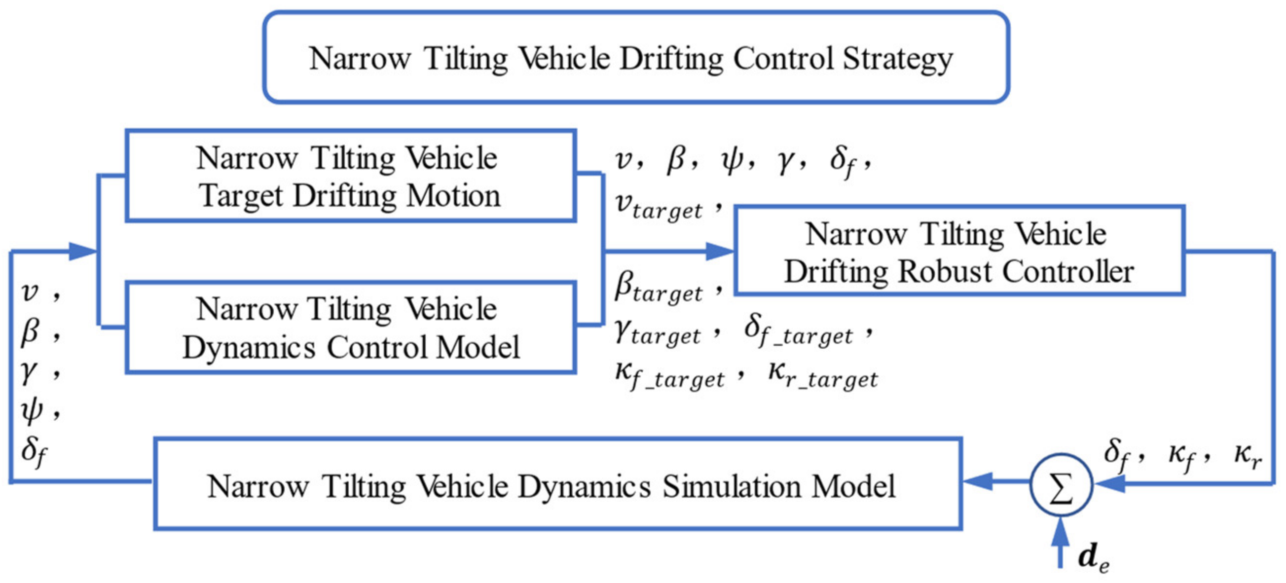
3. Narrow Tilting Vehicle Drifting Controller Design

A block scheme of the narrow tilting vehicle drifting control strategy is shown as Figure 6. Considering uncertain extern disturbances, ${\mathit{d}}_{\mathit{e}}$, the narrow tilting vehicle drifting controller is designed based on robust theory to realize the target drifting motion, including the target velocity $v_{target}$, the target sideslip angle ${\beta }_{target}$, the target yaw rate ${\gamma }_{target}$, the target steering angle ${\delta }_{f\_target}$, the target longitudinal slip ratio of the front axle ${\kappa }_{f\_target}$, and the target longitudinal slip ratio of the rear axle, ${\kappa }_{r\_target}$.

3.1. Controller System State-Space Expression

According to the above, the narrow tilting vehicle can be described as Equation (12).

$$\left[\begin{array}{c}\dot{v}\\ \dot{\beta }\\ \dot{\gamma }\\ \psi \end{array}\right]=\left[\begin{array}{cccc}\frac{\partial \dot{v}}{\partial v}& \frac{\partial \dot{v}}{\partial \beta }& \frac{\partial \dot{v}}{\partial \gamma }& 0\\ \frac{\partial \dot{\beta }}{\partial v}& \frac{\partial \dot{\beta }}{\partial \beta }& \frac{\partial \dot{\beta }}{\partial \gamma }& 0\\ \frac{\partial \dot{\gamma }}{\partial v}& \frac{\partial \dot{\gamma }}{\partial \beta }& \frac{\partial \dot{\gamma }}{\partial \gamma }& 0\\ \frac{\partial \psi }{\partial v}& 0& 0& 0\end{array}\right]\left[\begin{array}{c}v\\ \beta \\ \gamma \\ \mathsf{\Psi }\end{array}\right]+\left[\begin{array}{ccc}\frac{\partial \dot{v}}{\partial {\delta }_f}& \frac{\partial \dot{v}}{\partial {\kappa }_f}& \frac{\partial \dot{v}}{\partial {\kappa }_r}\\ \frac{\partial \dot{\beta }}{\partial {\delta }_f}& \frac{\partial \dot{\beta }}{\partial {\kappa }_f}& \frac{\partial \dot{\beta }}{\partial {\kappa }_r}\\ \frac{\partial \dot{\gamma }}{\partial {\delta }_f}& \frac{\partial \dot{\gamma }}{\partial {\kappa }_f}& \frac{\partial \dot{\gamma }}{\partial {\kappa }_r}\\ \frac{\partial \psi }{\partial {\delta }_f}& 0& 0\end{array}\right]\left[\begin{array}{c}{\delta }_f\\ {\kappa }_f\\ {\kappa }_r\end{array}\right],$$

(12)

where $\mathsf{\Psi }$ is the integral value of the rolling angle $\psi$, and

$$\frac{\partial \dot{v}}{\partial v}=-\frac{2C_d{A}_{f}v{\cos }^3\beta }{21.15m}+\frac{{\widehat{C}}_{yfl}+{\widehat{C}}_{yfr}}{m}\left(-\sin {\delta }_f\cos \beta +\cos {\delta }_f\sin \beta \right)\times \frac{\partial {\alpha }_f}{\partial v}+\frac{\left({\widehat{C}}_{yrl}-{\widehat{C}}_{yrr}\right)\sin \beta }{m}\times \frac{\partial {\alpha }_r}{\partial v},$$

$$\begin{array}{ll}\frac{\partial \dot{v}}{\partial \beta }& =\frac{3C_d{A}_f{v}^2{\cos }^2\beta \sin \beta }{21.15m}+\left(\frac{F_{xfl}+F_{xfr}}{m}-\frac{{\widehat{C}}_{yfl}+{\widehat{C}}_{yfr}}{m}\times \frac{\partial {\alpha }_f}{\partial \beta }\right)\left(-\cos {\delta }_f\sin \beta +\sin {\delta }_f\cos \beta \right)\\ & +\frac{F_{yfl}+F_{yfr}}{m}\left(\sin {\delta }_f\sin \beta +\cos {\delta }_f\cos \beta \right)-\left(\frac{F_{xrl}+F_{xrr}}{m}-\frac{{\widehat{C}}_{yrl}+{\widehat{C}}_{yrr}}{m}\times \frac{\partial {\alpha }_r}{\partial \beta }\right)\sin \beta +\frac{\left(F_{yrl}+F_{yrr}\right)\cos \beta }{m},\end{array}$$

$$\begin{array}{ll}\frac{\partial \dot{v}}{\partial \beta }& =\frac{3C_d{A}_f{v}^2{\cos }^2\beta \sin \beta }{21.15m}+\left(\frac{F_{xfl}+F_{xfr}}{m}-\frac{{\widehat{C}}_{yfl}+{\widehat{C}}_{yfr}}{m}\times \frac{\partial {\alpha }_f}{\partial \beta }\right)\left(-\cos {\delta }_f\sin \beta +\sin {\delta }_f\cos \beta \right)\\ & +\frac{F_{yfl}+F_{yfr}}{m}\left(\sin {\delta }_f\sin \beta +\cos {\delta }_f\cos \beta \right)-\left(\frac{F_{xrl}+F_{xrr}}{m}-\frac{{\widehat{C}}_{yrl}+{\widehat{C}}_{yrr}}{m}\times \frac{\partial {\alpha }_r}{\partial \beta }\right)\sin \beta +\frac{\left(F_{yrl}+F_{yrr}\right)\cos \beta }{m},\end{array}$$

$$\frac{\partial \dot{v}}{\partial \gamma }=\frac{{\widehat{C}}_{yfl}+{\widehat{C}}_{yfr}}{m}\left(-\sin {\delta }_f\cos \beta +\cos {\delta }_f\sin \beta \right)\times \frac{\partial {\alpha }_f}{\partial \gamma }+\frac{\left({\widehat{C}}_{yrl}+{\widehat{C}}_{yrr}\right)\sin \beta }{m}\times \frac{\partial {\alpha }_r}{\partial \gamma },$$

$$\frac{\partial \dot{v}}{\partial {\delta }_f}=\left(\frac{F_{xfl}+F_{xfr}}{m}+\frac{{\widehat{C}}_{yfl}+{\widehat{C}}_{yfr}}{m}\times \frac{\partial {\alpha }_f}{\partial {\delta }_f}\right)\left(-\sin {\delta }_f\cos \beta +\cos {\delta }_f\sin \beta \right)-\frac{F_{yfl}+F_{yfr}}{m}\left(\cos {\delta }_f\cos \beta +\sin {\delta }_f\sin \beta \right),$$

$$\frac{\partial \dot{v}}{\partial {\kappa }_f}=\frac{\left({\widehat{C}}_{xfl}+{\widehat{C}}_{xfr}\right)\left(\cos {\delta }_f\cos \beta +\sin {\delta }_f\sin \beta \right)}{m},$$

$$\begin{array}{ll}\frac{\partial \dot{\beta }}{\partial v}& =\frac{C_d{A}_f{\cos }^2\beta \sin \beta }{21.15m}+\frac{F_{xfl}+F_{xfr}}{m{v}^2}\left(-\sin {\delta }_f\cos \beta +\cos {\delta }_f\sin \beta \right)+\frac{F_{yfl}+F_{yfr}}{m{v}^2}\left(-\cos {\delta }_f\cos \beta -\sin {\delta }_f\sin \beta \right)\\ & +\frac{{\widehat{C}}_{yfl}+{\widehat{C}}_{yfr}}{mv}\left(\cos {\delta }_f\cos \beta +\sin {\delta }_f\sin \beta \right)\times \frac{\partial {\alpha }_f}{\partial v}+\frac{\left({\widehat{C}}_{yrl}+{\widehat{C}}_{yrr}\right)\cos \beta }{mv}\times \frac{\partial {\alpha }_r}{\partial v}+\frac{\left(F_{xrl}+F_{xrr}\right)\sin \beta }{m{v}^2}-\frac{\left(F_{yrl}+F_{yrr}\right)\cos \beta }{m{v}^2},\end{array}$$

$$\begin{array}{ll}\frac{\partial \dot{\beta }}{\partial \beta }& =\frac{C_d{A}_{f}v{\cos }^3\beta }{21.15m}-\frac{2C_d{A}_{f}v{\sin }^2\beta \cos \beta }{21.15m}-\left(\frac{F_{xfl}+F_{xfr}}{mv}-\frac{{\widehat{C}}_{yfl}+{\widehat{C}}_{yfr}}{mv}\times \frac{\partial {\alpha }_f}{\partial \beta }\right)\left(\sin {\delta }_f\sin \beta +\cos {\delta }_f\cos \beta \right)\\ & +\frac{F_{yfl}+F_{yfr}}{mv}\left(-\cos {\delta }_f\sin \beta +\sin {\delta }_f\cos \beta \right)-\left(\frac{F_{xrl}+F_{xrr}}{mv}-\frac{{\widehat{C}}_{yrl}+{\widehat{C}}_{yrr}}{mv}\times \frac{\partial {\alpha }_r}{\partial \beta }\right)\cos \beta -\frac{\left(F_{yrl}+F_{yrr}\right)\sin \beta }{mv},\end{array}$$

$$\frac{\partial \dot{\beta }}{\partial \gamma }=-1+\frac{{\widehat{C}}_{yfl}+{\widehat{C}}_{yfr}}{mv}\left(\cos {\delta }_f\cos \beta +\sin {\delta }_f\sin \beta \right)\times \frac{\partial {\alpha }_f}{\partial \gamma }+\frac{\left({\widehat{C}}_{yrl}+{\widehat{C}}_{yrr}\right)\cos \beta }{mv}\times \frac{\partial {\alpha }_r}{\partial \gamma },$$

$$\frac{\partial \dot{\beta }}{\partial {\delta }_f}=\left(\frac{F_{xf}}{mv}+\frac{{\widehat{C}}_{yfl}+{\widehat{C}}_{yfr}}{mv}\times \frac{\partial {\alpha }_f}{\partial {\delta }_f}\right)\left(\cos {\delta }_f\cos \beta +\sin {\delta }_f\sin \beta \right)+\frac{F_{yf}}{mv}\left(-\sin {\delta }_f\cos \beta +\cos {\delta }_f\sin \beta \right),$$

$$\frac{\partial \dot{\beta }}{\partial {\kappa }_f}=\frac{{\widehat{C}}_{xfl}+{\widehat{C}}_{xfr}}{mv}\left(\sin {\delta }_f\cos \beta -\cos {\delta }_f\sin \beta \right), \frac{\partial \dot{\beta }}{\partial {\kappa }_r}=-\frac{\left({\widehat{C}}_{xrl}+{\widehat{C}}_{xrr}\right)\sin \beta }{mv},$$

$$\frac{\partial \dot{\gamma }}{\partial v}=\frac{l_f\left({\widehat{C}}_{yfl}+{\widehat{C}}_{yfr}\right)}{I_z}\cos {\delta }_f\times \frac{\partial {\alpha }_f}{\partial v}-\frac{l_r\left({\widehat{C}}_{yrl}+{\widehat{C}}_{yrr}\right)}{I_z}\times \frac{\partial {\alpha }_r}{\partial v}+\frac{w_f\left({\widehat{C}}_{yfl}-{\widehat{C}}_{yfr}\right)}{2I_z}\sin {\delta }_f\times \frac{\partial {\alpha }_f}{\partial v},$$

$$\frac{\partial \dot{\gamma }}{\partial \beta }=\frac{l_f\left({\widehat{C}}_{yfl}+{\widehat{C}}_{yfr}\right)}{I_z}\cos {\delta }_f\times \frac{\partial {\alpha }_f}{\partial \beta }-\frac{l_r\left({\widehat{C}}_{yrl}+{\widehat{C}}_{yrr}\right)}{I_z}\times \frac{\partial {\alpha }_r}{\partial \beta }+\frac{w_f\left({\widehat{C}}_{yfl}-{\widehat{C}}_{yfr}\right)}{2I_z}\sin {\delta }_f\times \frac{\partial {\alpha }_f}{\partial \beta },$$

$$\frac{\partial \dot{\gamma }}{\partial \gamma }=\frac{l_f\left({\widehat{C}}_{yfl}+{\widehat{C}}_{yfr}\right)}{I_z}\cos {\delta }_f\times \frac{\partial {\alpha }_f}{\partial \gamma }-\frac{l_r\left({\widehat{C}}_{yrl}+{\widehat{C}}_{yrr}\right)}{I_z}\times \frac{\partial {\alpha }_r}{\partial \gamma }+\frac{w_f\left({\widehat{C}}_{yfl}-{\widehat{C}}_{yfr}\right)}{2I_z}\sin {\delta }_f\times \frac{\partial {\alpha }_f}{\partial \gamma },$$

$$\begin{array}{ll}\frac{\partial \dot{\gamma }}{\partial {\delta }_f}& =\frac{l_f\cos {\delta }_f}{I_z}\left(F_{xf}+\left({\widehat{C}}_{yfl}+{\widehat{C}}_{yfr}\right)\times \frac{\partial {\alpha }_f}{\partial {\delta }_f}\right)+\frac{w_f\cos {\delta }_f}{2I_z}\left(\left({\widehat{C}}_{yfl}-{\widehat{C}}_{yfr}\right)\left({\alpha }_f-{\widehat{\alpha }}_f\right)+\left({\widehat{F}}_{yfl}-{\widehat{F}}_{yfr}\right)\right)\\ & +\frac{w_f\sin {\delta }_f}{2I_z}\left(\left({\widehat{C}}_{xfl}-{\widehat{C}}_{xfr}\right)\left({\kappa }_f-{\widehat{\kappa }}_f\right)+\left({\widehat{F}}_{xfl}-{\widehat{F}}_{xfr}\right)+\left({\widehat{C}}_{yfl}-{\widehat{C}}_{yfr}\right)\times \frac{\partial {\alpha }_f}{\partial {\delta }_f}\right)-\frac{F_{yf}{l}_f}{I_z}\sin {\delta }_f,\end{array}$$

$$\frac{\partial \dot{\gamma }}{\partial {\kappa }_f}=\frac{l_f\left({\widehat{C}}_{xfl}+{\widehat{C}}_{xfr}\right)}{I_z}\sin {\delta }_f-\frac{w_f\left({\widehat{C}}_{xfl}-{\widehat{C}}_{xfr}\right)}{2I_z}\cos {\delta }_f, \frac{\partial \dot{\gamma }}{\partial {\kappa }_r}=-\frac{w_r\left({\widehat{C}}_{xrl}-{\widehat{C}}_{xrr}\right)}{2I_z},$$

$$\frac{\partial \psi }{\partial v}=-\frac{2v{\delta }_{f}g\left(l_f+l_r\right)}{g^2{\left(l_f+l_r\right)}^2+v^4{\delta }_f{}^2}, \frac{\partial \psi }{\partial {\delta }_f}=\frac{v^{2}g\left(l_f+l_r\right)}{g^2{\left(l_f+l_r\right)}^2+v^4{\delta }_f{}^2}$$

in which

$$\frac{\partial {\alpha }_f}{\partial v}=-\frac{\gamma l_f\cos \beta }{v^2+2v\gamma l_f\sin \beta +{\gamma }^2{l}_f{}^2}, \frac{\partial {\alpha }_f}{\partial \beta }=\frac{v^2+v\gamma l_f\sin \beta }{v^2+2v\gamma l_f\sin \beta +{\gamma }^2{l}_f{}^2},$$

$$\begin{gathered} \frac{\partial {\alpha }_f}{\partial \gamma }=\frac{v{l}_f\cos \beta }{v^2+2v\gamma l_f\sin \beta +{\gamma }^2{l}_f{}^2}, \frac{\partial {\alpha }_f}{\partial {\delta }_f}=-1, \\ \hspace{1em}\hspace{1em}\hspace{1em}\hspace{1em}\hspace{1em}\hspace{1em}\hspace{1em}\hspace{1em}\hspace{1em}\frac{\partial {\alpha }_r}{\partial v}=\frac{\gamma l_r\cos \beta }{v^2-2v\gamma l_r\sin \beta +{\gamma }^2{l}_r{}^2}, \end{gathered}$$

$$\frac{\partial {\alpha }_r}{\partial \beta }=\frac{v^2-\gamma l_r\cos \beta }{v^2-2v\gamma l_r\sin \beta +{\gamma }^2{l}_r{}^2}, \frac{\partial {\alpha }_r}{\partial \gamma }=\frac{-l_r}{v^2-2v\gamma l_r\sin \beta +{\gamma }^2{l}_r{}^2}.$$

The vehicle drifting motion is under the unique motion when forces between tires and the ground reach the maximum. According to the drifting motion characteristics, the status parameter values of the narrow tilting vehicle drifting motion can be calculated based on Equations (1)–(4) and play an important role as the target in the narrow tilting vehicle drifting realization. In order to simplify the controller design, considering the target drifting motion, the state-space expression of the narrow tilting dynamics model Equation (12) is derived as follows.

$$\dot{\mathit{x}}=\mathit{A}\mathit{x}+{\mathit{B}}_u\mathit{u},$$

(13)

where $\mathit{x}={\left[\begin{array}{ccc}v-v_{target} & \beta -{\beta }_{target}& \gamma -{\gamma }_{target}\end{array}\right]}^{\mathrm{T}}$ is the state vector of system, $\mathit{u}={\left[\begin{array}{ccc}{\delta }_f-{\delta }_{f\_target}& {\kappa }_f-{\kappa }_{f\_target}& {\kappa }_r-{\kappa }_{r\_target}\end{array}\right]}^{\mathrm{T}}$ is the control input of system, and coefficient matrices $\mathit{A}$ and ${\mathit{B}}_u$ are derived based on Equation (12) with the current and target motions.

3.2. Robust Controller

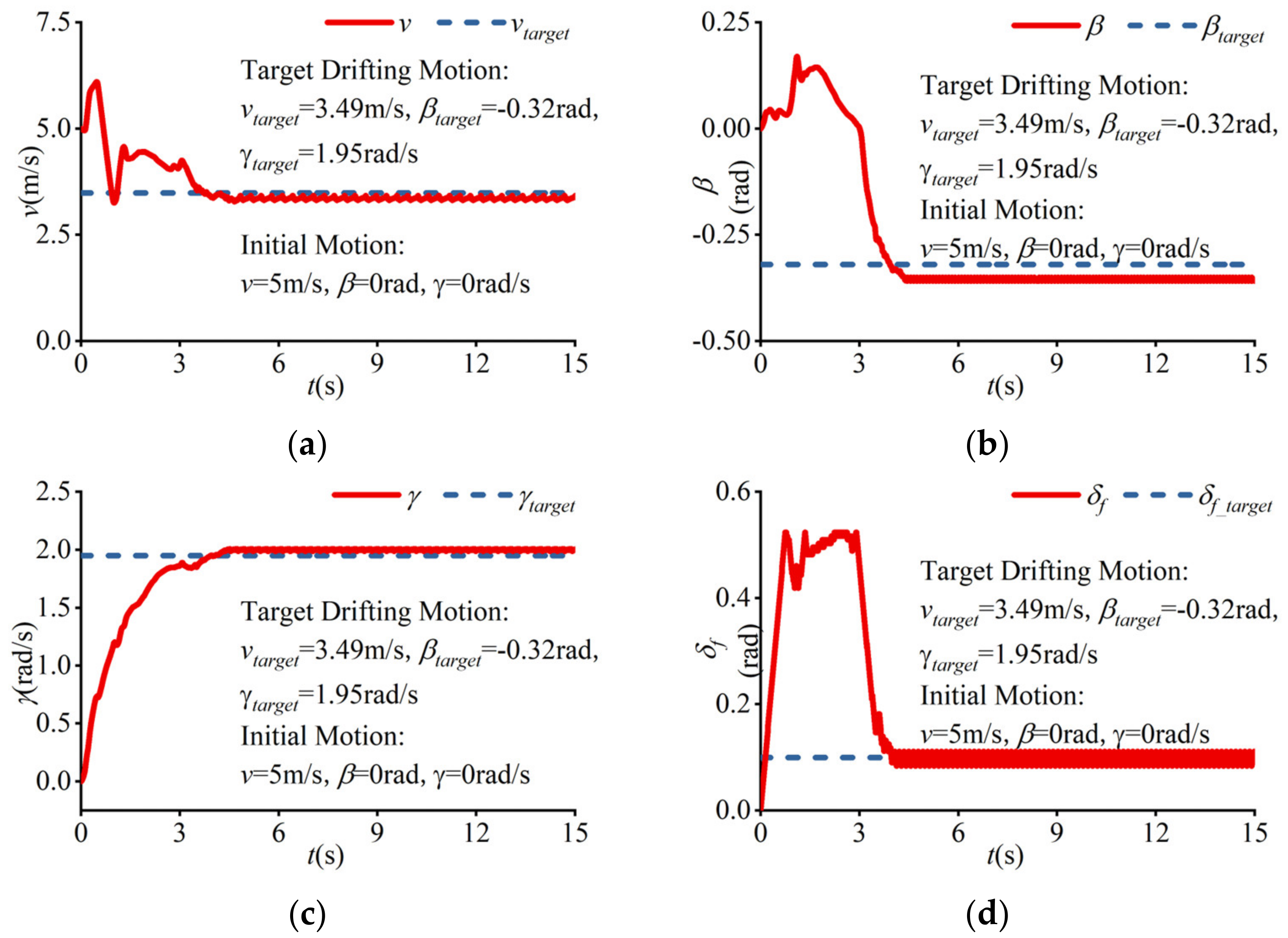
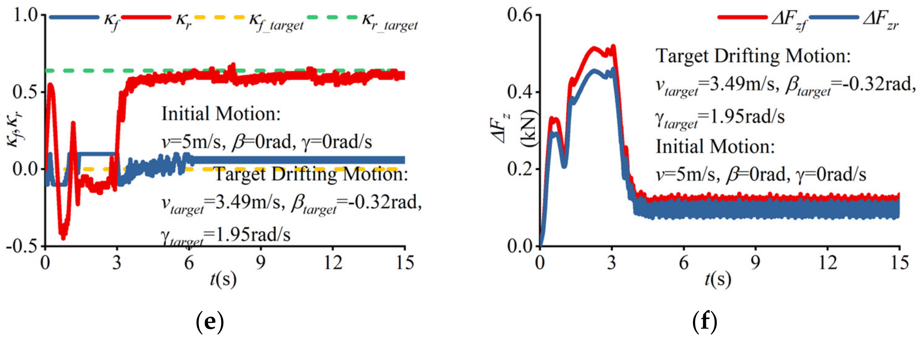
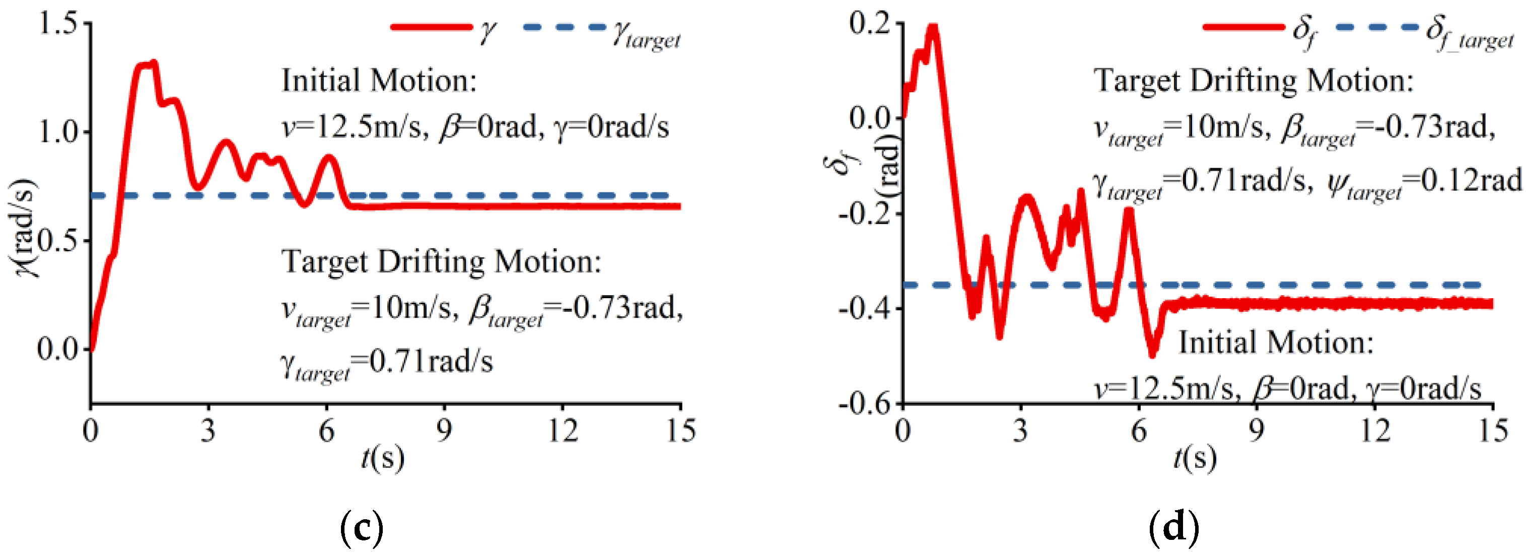
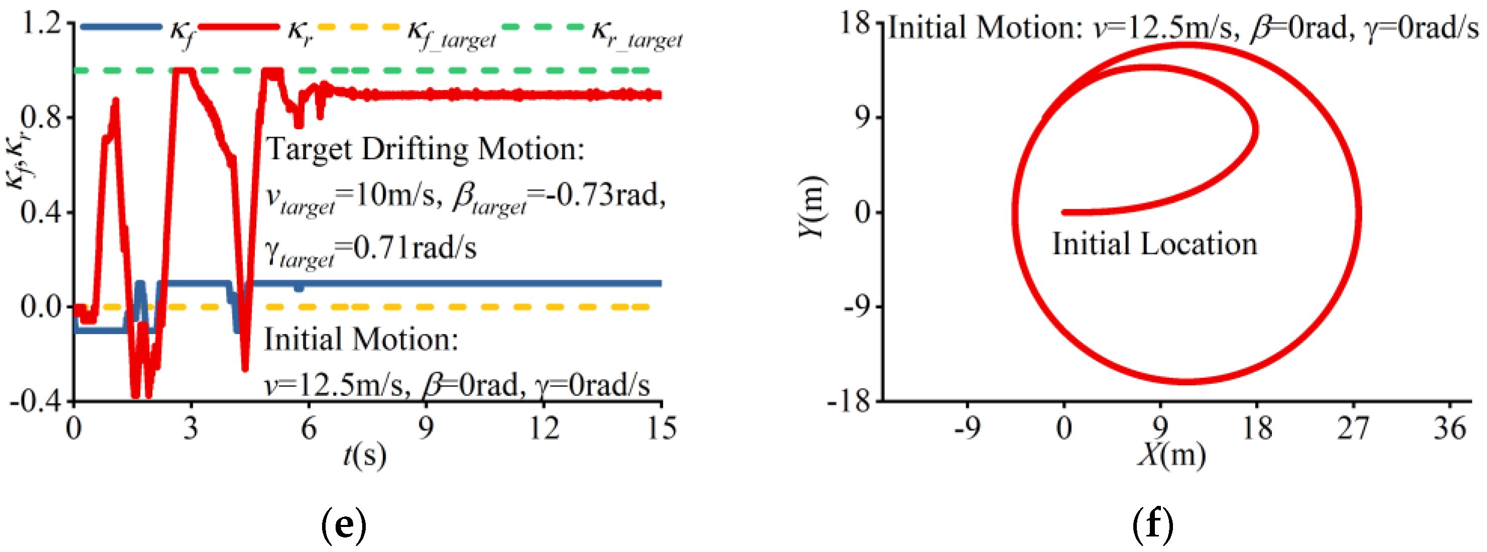
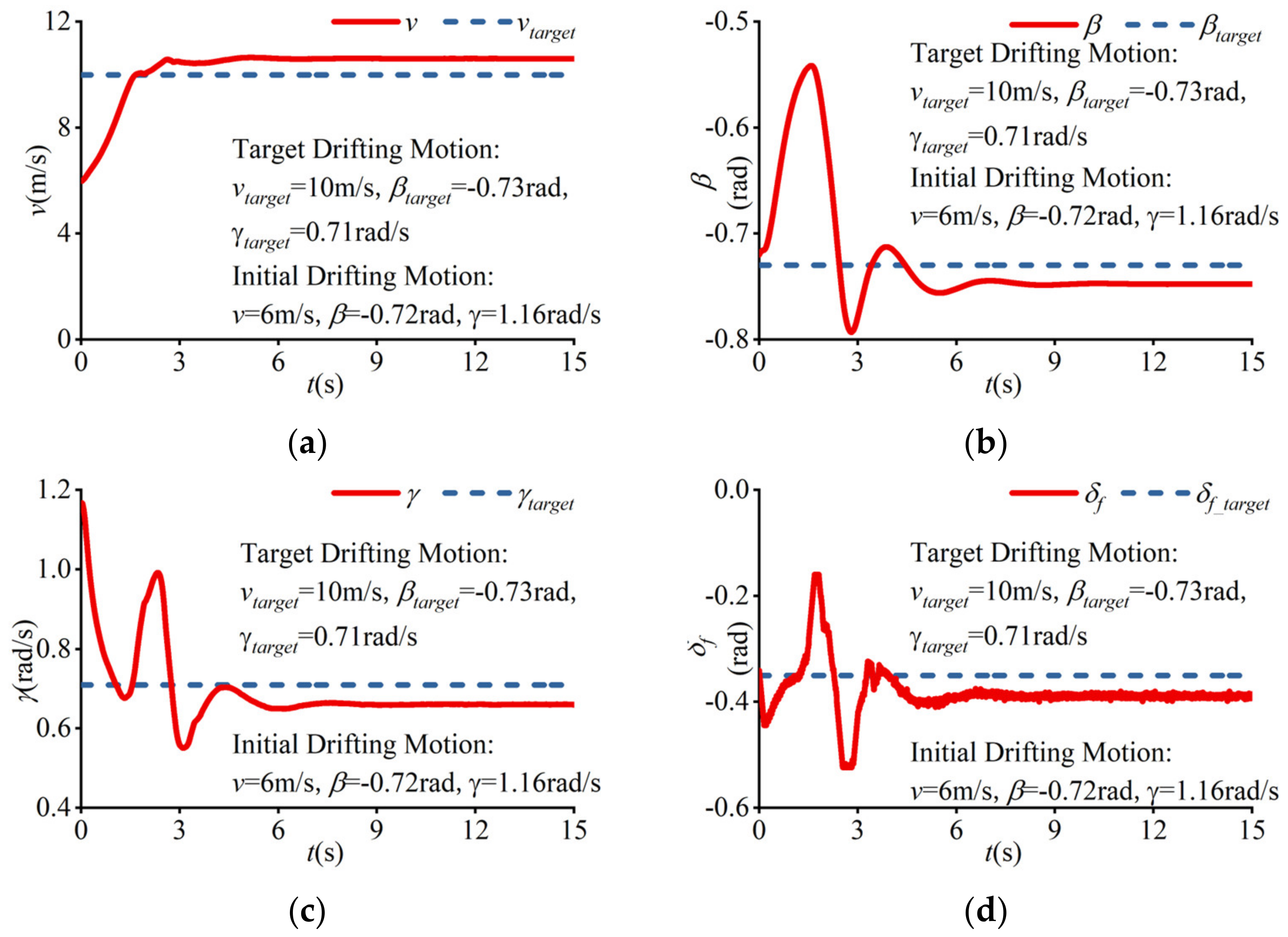
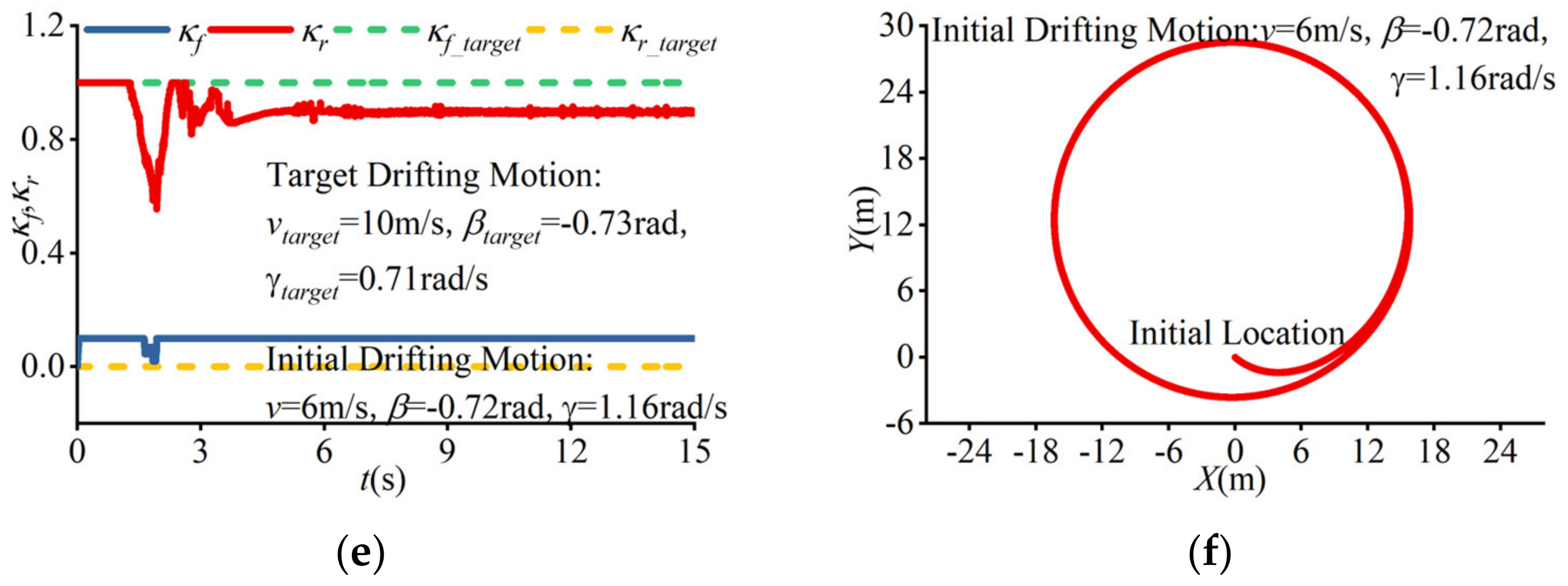
Combing Equation (13), the narrow tilting vehicle drifting control system with uncertain extern disturbances can be described as Equation (14).

$$\left\{\begin{array}{c}\dot{\mathit{x}}=\mathit{A}\mathit{x}+{\mathit{B}}_u\mathit{u}+{\mathit{B}}_d{\mathit{d}}_e\\ \mathit{y}=\mathit{x}\\ \mathit{z}={\left[{\mathit{C}}_Q,{\mathbf{0}}_{3\times 3}\right]}^{\mathrm{T}}\mathit{x}+{\left[{\mathbf{0}}_{3\times 3},{\mathit{C}}_R\right]}^{\mathrm{T}}\mathit{u}\end{array}\right.,$$

(14)

where $\mathit{y}$ is the measurement output of system, $\mathit{z}$ is the controlled output pf system, ${\mathit{d}}_e={\left[\begin{array}{ccc}{d}_{\delta }& d_f& d_r\end{array}\right]}^{\mathrm{T}}$ and $d_{\delta }$, $d_f$, and $d_r$ are uncertain extern disturbances concerned with inputs, the coefficient matrix ${\mathit{B}}_d$ expresses the correlation between the differential state vector and the disturbance vector, coefficient matrices ${\mathit{C}}_Q$ and ${\mathit{C}}_R$ are symmetric matrices and ${\mathit{C}}_Q>0$, and the symbol ${\mathbf{0}}_{3\times 3}$ expresses the null matrix with three rows and three columns.

The robust state-feedback control law is designed as:

$$\mathit{u}=\mathit{K}\mathit{x},$$

(15)

where $\mathit{K}$ is the control gain matrix.

The robust cost function is designed as:

$$\mathit{J}={\int }_0^t{\mathit{z}}^{\mathrm{T}}\mathit{z}\mathrm{d}t={\int }_0^t\left({\mathit{x}}^{\mathrm{T}}\mathit{Q}\mathit{x}+{\mathit{u}}^{\mathrm{T}}\mathit{R}\mathit{u}\right)\mathrm{d}t,$$

(16)

where weight matrices $\mathit{Q}$ and $\mathit{R},$ respectively, equal ${\mathit{C}}_Q{}^{\mathrm{T}}{\mathit{C}}_Q$ and ${\mathit{C}}_R{}^{\mathrm{T}}{\mathit{C}}_R$.

To ensure the antijamming capability of the narrow tilting vehicle drifting control system, it need be suppressed that the uncertain extern disturbances impact on the controller performance. Thus, the cost function in Equation (16) needs to satisfy the following:

$${\int }_0^t\left({\mathit{x}}^{\mathrm{T}}\mathit{Q}\mathit{x}+{\mathit{u}}^{\mathrm{T}}\mathit{R}\mathit{u}\right)\mathrm{d}t<{\rho }^2{\int }_0^t{\mathit{d}}_e{}^{\mathrm{T}}{\mathit{d}}_e\mathrm{d}t,$$

(17)

where $\rho$ is the scalar to express the anti-disturbance capability and $\rho >0$.

To guarantee the convergence of the control system towards the balance state, the Lyapunov stability is satisfied and the Lyapunov function and the derived function are selected as follows:

$$\mathit{L}={\mathit{x}}^{\mathrm{T}}\mathit{P}\mathit{x},$$

(18)

$$\dot{\mathit{L}}={\dot{\mathit{x}}}^{\mathrm{T}}\mathit{P}\mathit{x}+{\mathit{x}}^{\mathrm{T}}\mathit{P}\dot{\mathit{x}},$$

(19)

where the matrix $\mathit{P}$ is the positive definite symmetric matrix.

The Lyapunov derived function Equation (19) can be derived as:

$$\dot{\mathit{L}}={\mathit{\lambda }}^{\mathrm{T}}\left[\begin{array}{cc}{\mathit{P}}_s{}^{\mathrm{T}}+{\mathit{P}}_s& \mathit{P}{\mathit{B}}_d\\ {\mathit{B}}_d{}^{\mathrm{T}}\mathit{P}& {\mathbf{0}}_{3\times 3}\end{array}\right]\mathit{\lambda },$$

(20)

where the vector $\mathit{\lambda }$ is the set of the state vector and the uncertain extern disturbance vector and $\mathit{\lambda }={\left[{\mathit{x}}^{\mathrm{T}},{\mathit{d}}_e{}^{\mathrm{T}}\right]}^{\mathrm{T}}$, the matrix ${\mathit{P}}_s$ represents the operation $\mathit{P}\left(\mathit{A}+{\mathit{B}}_u\mathit{K}\right)$, and the matrix ${\mathbf{0}}_{3\times 3}$ expresses the null matrix with three rows and three columns.

The derived function of the cost function Equation (16) can be described as:

$${\mathit{x}}^{\mathrm{T}}\mathit{Q}\mathit{x}+{\mathit{u}}^{\mathrm{T}}\mathit{R}\mathit{u}-{\rho }^2{\mathit{d}}_e{}^{\mathrm{T}}{\mathit{d}}_e={\mathit{\lambda }}^{\mathrm{T}}\left[\begin{array}{cc}\mathit{Q}+{\mathit{K}}^{\mathrm{T}}\mathit{R}\mathit{K}& {\mathbf{0}}_{3\times 3}\\ {\mathbf{0}}_{3\times 3}& -{\rho }^2{\mathit{E}}_{3\times 3}\end{array}\right]\mathit{\lambda }$$

(21)

where the symbol ${\mathit{E}}_{3\times 3}$ expresses the unit matrix with three rows and three columns.

When combining Equations (20) and (21), the following equation can be obtained:

$$\dot{\mathit{L}}+{\mathit{x}}^{\mathrm{T}}\mathit{Q}\mathit{x}+{\mathit{u}}^{\mathrm{T}}\mathit{R}\mathit{u}-{\rho }^2{\mathit{d}}_e{}^{\mathrm{T}}{\mathit{d}}_e={\mathit{\lambda }}^{\mathrm{T}}\left[\begin{array}{cc}{\mathit{P}}_s{}^{\mathrm{T}}+{\mathit{P}}_s+\mathit{Q}+{\mathit{K}}^{\mathrm{T}}\mathit{R}\mathit{K}& \mathit{P}{\mathit{B}}_d\\ {\mathit{B}}_d{}^{\mathrm{T}}\mathit{P}& -{\rho }^2{\mathit{E}}_{3\times 3}\end{array}\right]\mathit{\lambda },$$

(22)

The result of the control system stability judgment can be obtained based on Equation (22), and the control system will be stable with uncertain external disturbances only if the symmetric matrix in Equation (22) satisfies the following:

$$\left[\begin{array}{cc}{\mathit{P}}_s{}^{\mathrm{T}}+{\mathit{P}}_s+\mathit{Q}+{\mathit{K}}^{\mathrm{T}}\mathit{R}\mathit{K}& \mathit{P}{\mathit{B}}_d\\ {\mathit{B}}_d{}^{\mathrm{T}}\mathit{P}& -{\rho }^2{\mathit{E}}_{3\times 3}\end{array}\right]<0,$$

(23)

Then, Equation (22) can be derived as:

$$\dot{\mathit{L}}+{\mathit{x}}^{\mathrm{T}}\mathit{Q}x+{\mathit{u}}^{\mathrm{T}}\mathit{R}\mathit{u}-{\rho }^2{\mathit{d}}_e{}^{\mathrm{T}}{\mathit{d}}_e\le 0,$$

(24)

Integrating Equation (24), the cost function satisfies the following:

$$\mathit{L}\le {\rho }^2{\int }_0^t{\mathit{d}}_e{}^{\mathrm{T}}{\mathit{d}}_e\mathrm{d}t-{\int }_0^t\left(x^{\mathrm{T}}\mathit{Q}x+{\mathit{u}}^{\mathrm{T}}\mathit{R}\mathit{u}\right)\mathrm{d}t+\mathit{L}\left(0\right)\le {\rho }^2{\int }_0^t{\mathit{d}}_e{}^{\mathrm{T}}{\mathit{d}}_e\mathrm{d}t+\mathit{L}\left(0\right)$$

(25)

Thus, the following can be derived:

$${\mathit{P}}_{min}||\mathit{x}|{|}^2\le {\mathit{x}}^{\mathrm{T}}\mathit{P}\mathit{x}\le {\rho }^2{\int }_0^t{\mathit{d}}_e{}^{\mathrm{T}}{\mathit{d}}_e\mathrm{d}t+\mathit{L}\left(0\right),$$

$$||\mathit{x}|{|}^2\le \frac{{\rho }^2{\int }_0^t{\mathit{d}}_e{}^{\mathrm{T}}{\mathit{d}}_e\mathrm{d}t+\mathit{L}\left(0\right)}{{\mathit{P}}_{min}},$$

(26)

According to the Schur complement theorem in [29], the following can be derived and Equation (23) can be transformed as Equation (27).

$$\left[\begin{array}{ccc}{\mathit{P}}_s{}^{\mathrm{T}}+{\mathit{P}}_s+\mathit{Q}& \mathit{P}{\mathit{B}}_d& {\mathit{K}}^{\mathrm{T}}{\mathit{C}}_R\\ {\mathit{B}}_d{}^{\mathrm{T}}\mathit{P}& -{\rho }^2{\mathit{E}}_{3\times 3}& {\mathbf{0}}_{3\times 3}\\ {\mathit{C}}_R\mathit{K}& {\mathbf{0}}_{3\times 3}& -{\mathit{E}}_{3\times 3}\end{array}\right]<0,$$

$$\left[\begin{array}{cccc}{\mathit{P}}_s{}^{\mathrm{T}}+{\mathit{P}}_s& \mathit{P}{\mathit{B}}_d& {\mathit{K}}^{\mathrm{T}}{\mathit{C}}_R& {\mathit{C}}_Q\\ {\mathit{B}}_d{}^{\mathrm{T}}\mathit{P}& -{\rho }^2{\mathit{E}}_{3\times 3}& {\mathbf{0}}_{3\times 3}& {\mathbf{0}}_{3\times 3}\\ {\mathit{C}}_R\mathit{K}& {\mathbf{0}}_{3\times 3}& -{\mathit{E}}_{3\times 3}& {\mathbf{0}}_{3\times 3}\\ {\mathit{C}}_Q& {\mathbf{0}}_{3\times 3}& {\mathbf{0}}_{3\times 3}& -{\mathit{E}}_{3\times 3}\end{array}\right]<0,$$

(27)

Because of the equations ${\mathit{P}}_s=\mathit{P}\left(\mathit{A}+{\mathit{B}}_u\mathit{K}\right)$ and ${\mathit{P}}_s{}^{\mathrm{T}}={\left(\mathit{A}+{\mathit{B}}_u\mathit{K}\right)}^{\mathrm{T}}\mathit{P}$, Equation (27) becomes the following:

$$\left[\begin{array}{cccc}\mathit{P}\left(\mathit{A}+{\mathit{B}}_u\mathit{K}\right)+{\left(\mathit{A}+{\mathit{B}}_u\mathit{K}\right)}^{\mathrm{T}}\mathit{P}& \mathit{P}{\mathit{B}}_d& {\mathit{K}}^{\mathrm{T}}{\mathit{C}}_R& {\mathit{C}}_Q\\ {\mathit{B}}_d{}^{\mathrm{T}}\mathit{P}& -{\rho }^2{\mathit{E}}_{3\times 3}& {\mathbf{0}}_{3\times 3}& {\mathbf{0}}_{3\times 3}\\ {\mathit{C}}_R\mathit{K}& {\mathbf{0}}_{3\times 3}& -{\mathit{E}}_{3\times 3}& {\mathbf{0}}_{3\times 3}\\ {\mathit{C}}_Q& {\mathbf{0}}_{5\times 3}& {\mathbf{0}}_{3\times 3}& -{\mathit{E}}_{3\times 3}\end{array}\right]<0,$$

(28)

To solve the two unknown variable matrices $\mathit{P}$ and $\mathit{K}$ simply, both sides of Equation (28) are multiplied by the matrix $\mathit{S}=diag\left\{\begin{array}{cccc}{\mathit{P}}^{-1}& {\mathit{E}}_{3\times 3}& {\mathit{E}}_{3\times 3}& {\mathit{E}}_{3\times 3}\end{array}\right\}$, and the solution can be calculated by the following LMIs.

$$\begin{gathered} \mathit{P}>0, \\ \left[\begin{array}{cccc}\mathit{A}{\mathit{P}}^{-1}+{\mathit{B}}_u\mathit{K}{\mathit{P}}^{-1}+{\mathit{P}}^{-1}{\mathit{A}}^{\mathrm{T}}+{\mathit{P}}^{-1}{\mathit{K}}^{\mathrm{T}}{\mathit{B}}_u{}^{\mathrm{T}}& {\mathit{B}}_d& {\mathit{P}}^{-1}{\mathit{K}}^{\mathrm{T}}{\mathit{C}}_R& {\mathit{P}}^{-1}{\mathit{C}}_Q\\ {\mathit{B}}_d{}^{\mathrm{T}}& -{\rho }^2{\mathit{E}}_{3\times 3}& {\mathbf{0}}_{3\times 3}& {\mathbf{0}}_{3\times 3}\\ {\mathit{C}}_R\mathit{K}{\mathit{P}}^{-1}& {\mathbf{0}}_{3\times 3}& -{\mathit{E}}_{3\times 3}& {\mathbf{0}}_{3\times 3}\\ {\mathit{C}}_Q{\mathit{P}}^{-1}& {\mathbf{0}}_{3\times 3}& {\mathbf{0}}_{3\times 3}& -{\mathit{E}}_{3\times 3}\end{array}\right]<0, \end{gathered}$$

(29)

The inverse operation and the multiplied operation related to the unknow matrices are expressed as the following for the simplified calculation of Equation (29).

$${\mathit{R}}_1={\mathit{P}}^{-1},$$

(30)

$${\mathit{R}}_2=\mathit{K}{\mathit{P}}^{-1},$$

(31)

Thus, Equation (29) can be derived as Equation (32), and the solution of the equation can be transformed to the solution of Equation (28).

$$\begin{array}{c}{\mathit{R}}_1>0,\\ \left[\begin{array}{cccc}\mathit{A}{\mathit{R}}_1+{\mathit{B}}_u{\mathit{R}}_2+{\mathit{R}}_1{\mathit{A}}^{\mathrm{T}}+{\mathit{R}}_2{}^{\mathrm{T}}{\mathit{B}}_u{}^{\mathrm{T}}& {\mathit{B}}_d& {\mathit{R}}_2{}^{\mathrm{T}}{\mathit{C}}_R& {\mathit{R}}_1{\mathit{C}}_Q\\ {\mathit{B}}_d{}^{\mathrm{T}}& -{\rho }^2{\mathit{E}}_{3\times 3}& {\mathbf{0}}_{3\times 3}& {\mathbf{0}}_{3\times 3}\\ {\mathit{C}}_R{\mathit{R}}_2& {\mathbf{0}}_{3\times 3}& -{\mathit{E}}_{3\times 3}& {\mathbf{0}}_{3\times 3}\\ {\mathit{C}}_Q{\mathit{R}}_1& {\mathbf{0}}_{3\times 3}& {\mathbf{0}}_{3\times 3}& -{\mathit{E}}_{3\times 3}\end{array}\right]<0,\end{array}$$

(32)

According the solution, the control gain matrix $K$ can be calculated and the actual control parameters can be obtained as Equation (33).

$${\left[{\delta }_f,{\kappa }_f,{\kappa }_r\right]}^{\mathrm{T}}=\mathit{K}\mathit{x}+{\left[{\delta }_{f{\_}_{target}},{\kappa }_{f_{\_target}},{\kappa }_{r{\_}_{target}}\right]}^{\mathrm{T}},$$

(33)

4. Narrow Tilting Vehicle Drifting Control Simulation Results

The narrow tilting vehicle main parameters are shown in

Table 1. The main parameters of the narrow tilting vehicle.

$\mathit{m}$	${\mathit{m}}_{\mathit{b}}$	${\mathit{I}}_{\mathit{z}}$	${\mathit{l}}_{\mathit{f}}$	${\mathit{l}}_{\mathit{r}}$	${\mathit{w}}_{\mathit{r}}$	${\mathit{w}}_{\mathit{f}}$	${\mathit{h}}_{\mathit{g}}$
237.1 kg	195.4 kg	243.2 kg∙m2	0.73 m	0.80 m	0.68 m	0.70 m	0.42 m

and the maximum steering angle is 0.52 rad in practice. The satisfying performance of the robust Controller is verified with uncertain disturbances in MATLAB/Simulink. The simulation system is established based on Equations (1)–(4) and Equations (6)–(10), and the uncertain external disturbances are described as random numbers and the coefficient matrix ${\mathit{B}}_d$ equals the coefficient matrix ${\mathit{B}}_u$.

The narrow tilting vehicle drifting controller is calculated and obtained with the steady-state target drifting motion in

Table 2. Target drifting motion groups.

Target Group	${\mathit{v}}_{\mathit{t}\mathit{a}\mathit{r}\mathit{g}\mathit{e}\mathit{t}}$	${\mathit{\beta }}_{\mathit{t}\mathit{a}\mathit{r}\mathit{g}\mathit{e}\mathit{t}}$	${\mathit{\gamma }}_{\mathit{t}\mathit{a}\mathit{r}\mathit{g}\mathit{e}\mathit{t}}$	${\mathit{\delta }}_{\mathit{f}{\_}_{\mathit{t}\mathit{a}\mathit{r}\mathit{g}\mathit{e}\mathit{t}}}$	${\mathit{\kappa }}_{{\mathit{f}}_{\_\mathit{t}\mathit{a}\mathit{r}\mathit{g}\mathit{e}\mathit{t}}}$	${\mathit{\kappa }}_{\mathit{r}{\_}_{\mathit{t}\mathit{a}\mathit{r}\mathit{g}\mathit{e}\mathit{t}}}$	$\mathit{\mu }$
(1)	3.49 m/s	−0.32 rad	1.95 rad/s	0.1 rad	0	0.64	0.75
(2)	10 m/s	−0.73 rad	0.71 rad/s	−0.35 rad	0	1	0.75

, which can be obtained by the analysis of the narrow tilting vehicle drifting motion state parameters in the condition that tire forces reach the maximum. Furthermore, the narrow tilting vehicle drifting controller starts to work under different initial motion conditions in

Table 3. Initial motion groups.

Initial Group	$\mathit{v}$	$\mathit{\beta }$	$\mathit{\gamma }$	${\mathit{\delta }}_{\mathit{f}}$	${\mathit{\kappa }}_{\mathit{f}}$	${\mathit{\kappa }}_{\mathit{r}}$	$\mathit{\mu }$
(1)	5 m/s	0 rad	0 rad/s	0 rad	0	0	0.75
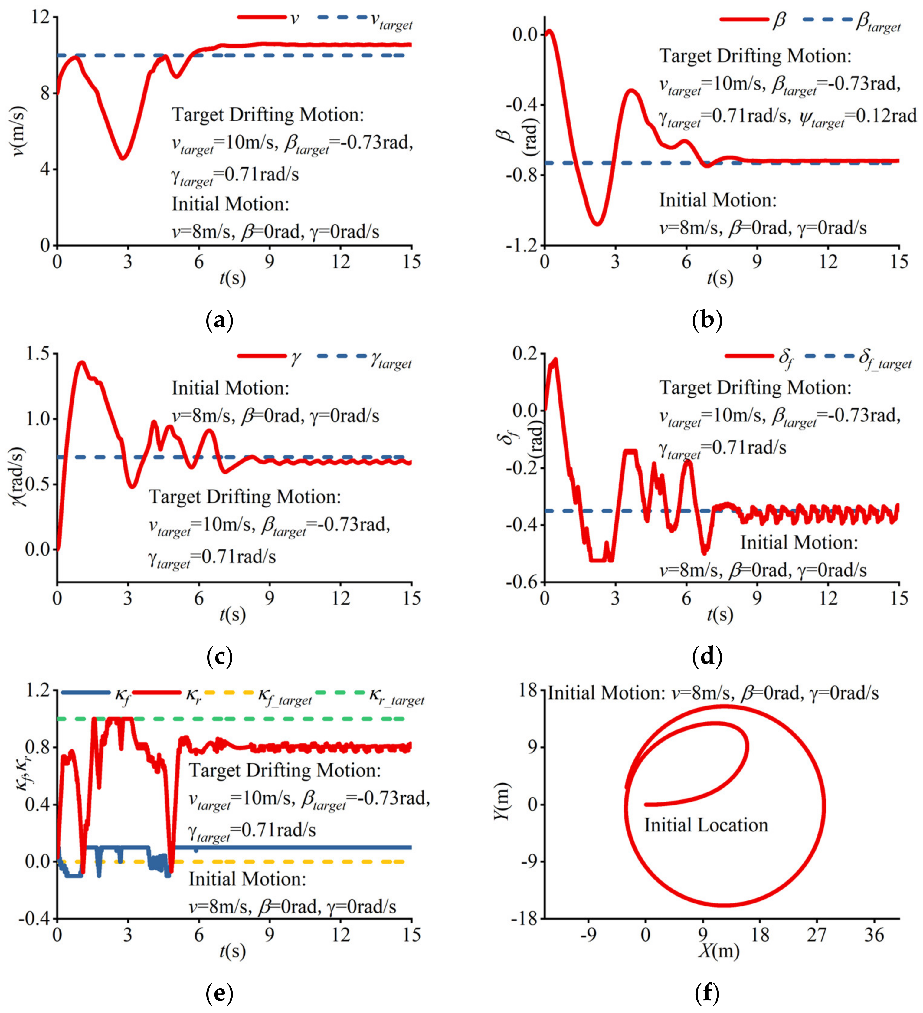
(2)	8 m/s	0 rad	0 rad/s	0 rad	0	0	0.75
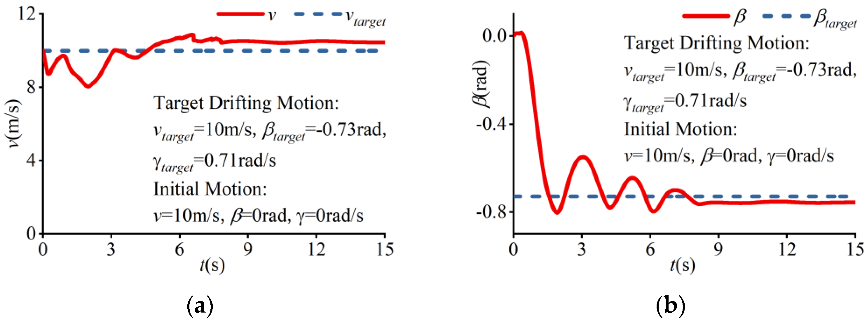
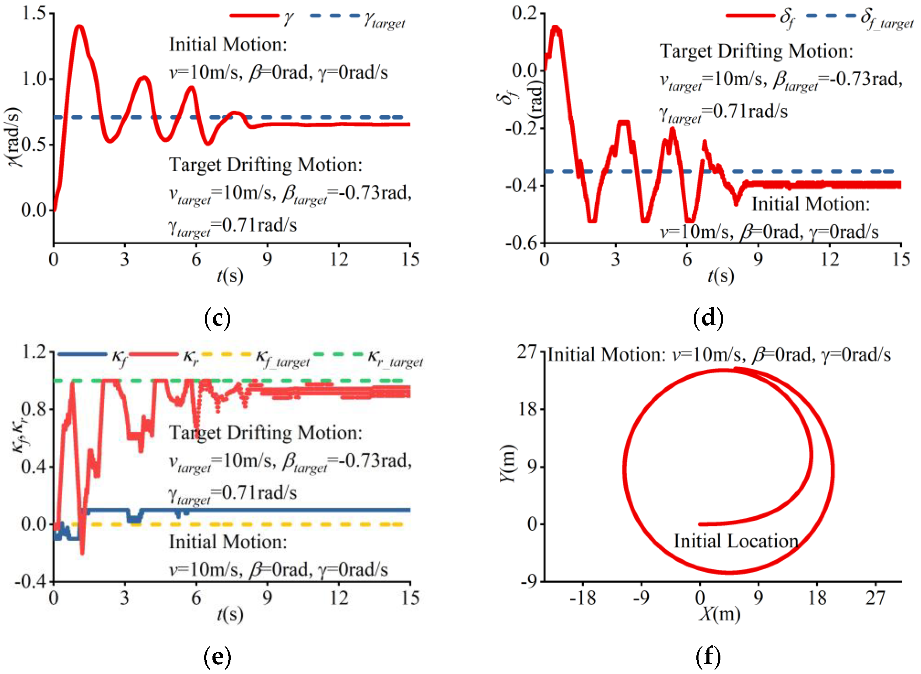
(3)	10 m/s	0 rad	0 rad/s	0 rad	0	0	0.75
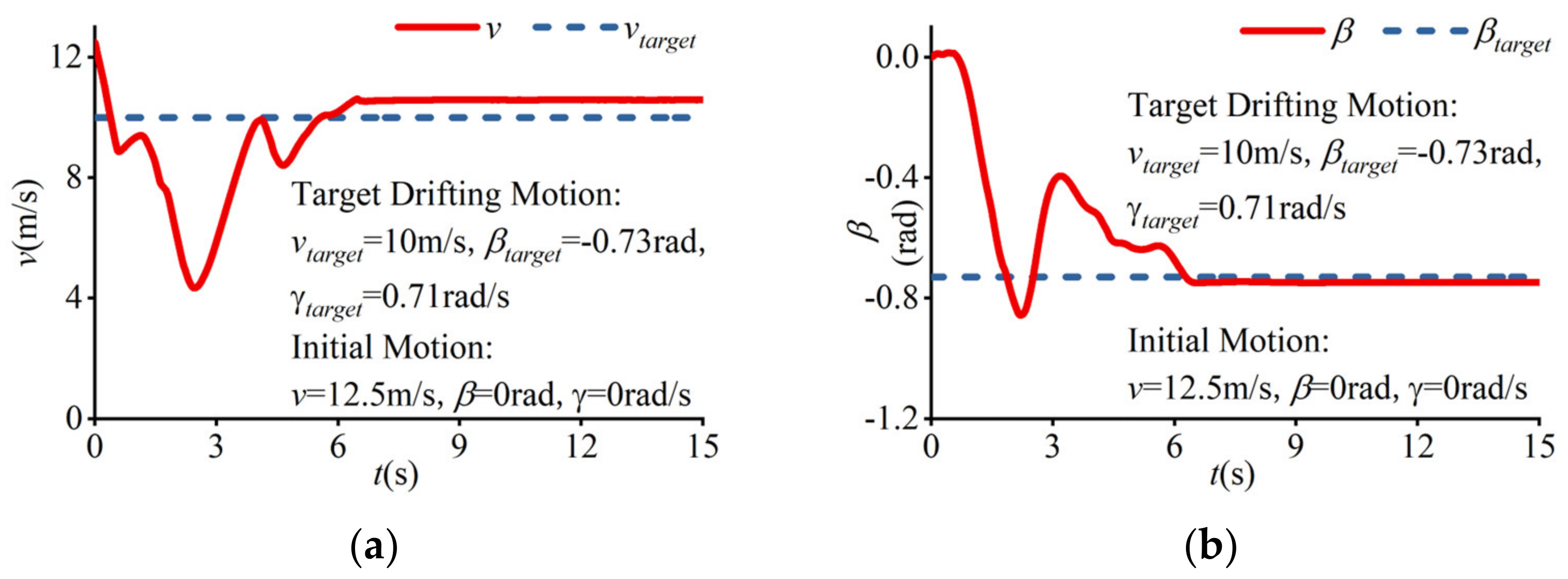
(4)	12.5 m/s	0 rad	0 rad/s	0 rad	0	0	0.75
(5) *	6 m/s	−0.72 rad	1.16 rad/s	−0.34 rad	0	1	0.75

* A drifting motion.

to verify that the designed controller has good performance in different conditions.

Considering the steering angle and longitudinal slip ratio ranges in practice, their amplitudes and gains are limited in simulation. The designed controller is used to realize target drifting motions in different initial motion conditions. The simulation results are shown in Figure 7, Figure 8, Figure 9, Figure 10 and Figure 11, including velocities, sideslip angles, yaw rates, steering angles, longitudinal slip ratios, and position modifications, which suggests the designed controller has a good performance. In Figure 7, the target drifting motion is a typical drifting working condition with a large yaw rate, and the initial motion is a uniform linear motion, and the simulation result suggests the designed controller can realize the drifting motion with a small turning radius at a low velocity and a large yaw rate. Figure 7f suggests that there are smaller vertical load transforms of the active rolling than the normal, which means the narrow tilting vehicle is safer than the normal narrow vehicle in the drifting motion. In Figure 8, Figure 9 and Figure 10, the target drifting motion is another typical drifting working condition with the maximum longitudinal slip ratio of the rear axle wheels, and the initial motions are uniform linear motions with different velocities, and the simulation results suggest that the designed controller can realize the same target drifting motion with different initial velocities. In Figure 11, the initial motion is a steady-state drifting motion different from others, and the simulation result suggests the designed controller can switch implementations for different drifting motions. Because the controller dynamics model is simplified based on the simulation model, there are some distances from the final state values and the target state values in Figure 7, Figure 8, Figure 9, Figure 10 and Figure 11, but most relative errors inspected are less than 5%, and the maximum relative error is less than 10%. In addition, because of the significant differences between the target and initial motions and the amplitude and gain limitations of the control inputs, the designed controller needs some implementation time and some slight adjustments for the final state values to accomplish the target motions.

The narrow tilting vehicle with the designed robust drifting controller can realize different target drifting motions in different initial states. The designed controller can realize the narrow tilting vehicle drifting motions with uncertain external disturbances and with the consideration of not only the target drifting state parameters, but also the target drifting control parameters. The controller realizes a typical drifting motion with a large yaw rate, and the final trajectory is a circle with a small turning radius at a low velocity. Additionally, the controller also can realize another typical drifting motion with a large longitudinal slip ratio of the rear axle wheels, and the initial states include different uniform linear motions and a drifting motion. The simulation results suggest that the designed controller makes it easy for the narrow tilting vehicle to realize different drifting motions with uncertain external disturbances.

5. Conclusions

This paper researches the drifting motion independent control of the narrow tilting vehicle based on a robust theory with uncertain external disturbances. The drifting control of the narrow titling vehicle is significant to improve traffic safety based on a narrow tilting vehicle and drifting motion characteristics. According to the active rolling chrematistics, the narrow tilting dynamic model is established to describe the characteristics, and simplified expressions are used in the drifting controller design. With uncertain external disturbances, the drifting controller of the narrow tilting vehicle is designed based on robust theory and calculated by the LMIs to realize narrow tilting vehicle drifting motions and tire limit operations. The controller is tested to realize different drifting motions with different initial motions, which suggests that the controller has a good performance of drifting motion realizations with a wide application. The narrow tilting vehicle drifting control can make the utmost of the vehicle’s dynamic performance and improve driving safety, especially when tires reach the maximum, which is worth further research.

References

- China Association of Automobile Manufacturers. Available online: http://en.caam.org.cn/Index/show/catid/57/id/1864.html (accessed on 15 November 2022).
- World Health Organization. Available online: https://www.who.int/news-room/fact-sheets/detail/the-top-10-causes-of-death (accessed on 9 December 2020).
- World Health Organization. Available online: https://www.who.int/publications/i/item/9789241565684 (accessed on 17 June 2018).
- World Health Organization. Available online: https://www.who.int/zh/news/item/30-06-2022-new-political-declaration-to-halve-road-traffic-deaths-and-injuries-by-2030-is-a-milestone-achievement (accessed on 30 June 2022).
- Wu, J.; Tian, Y.; Walker, P.; Li, Y. Attenuation Reference Model Based Adaptive Speed Control Tactic for Automatic Steering System. Mech. Syst. Signal Process. 2021, 156, 107631. [Google Scholar] [CrossRef]
- Zhang, Z.; Li, Y.; Yu, Y.; Zhang, Z.; Zheng, L. Study on Local Path Planning and Tracking Algorithm of Intelligent Vehicle in Complex Dynamics Environment. China J. Highw. Transp. 2022, 35, 372–386. [Google Scholar] [CrossRef]
- Wu, J.; Zhang, J.; Tian, Y.; Li, L. A Novel Adaptive Steering Torque Control Approach for Human-Machine-Cooperation Autonomous Vehicles. IEEE Trans. Transp. Electrif. 2021, 7, 2516–2525. [Google Scholar] [CrossRef]
- Claveau, F.; Chevrel, P.; Mourad, L. Non-Linear Control of a Narrow Tilting Vehicle. In Proceedings of the 2014 IEEE International Conference on Systems, Man, and Cybernetics, San Diego, CA, USA, 5–8 October 2014. [Google Scholar] [CrossRef] [Green Version]
- Mourad, F.; Claveau, F.; Chevrel, P. Design of a Two DOF Gain Scheduled Frequency Shaped LQ Controller for Narrow Tilting Vehicles. In Proceedings of the 2012 American Control Conference, Montreal, Canada, 27–29 June 2012. [Google Scholar] [CrossRef]
- Barker, M.; Drew, B.; Darling, J.; Edge, K.A.; Owen, G.W. Steady-State Steering of a Tilting Three-Wheeled Vehicle. Veh. Syst. Dyn. 2010, 48, 815–830. [Google Scholar] [CrossRef]
- Rajamani, R.; Gohl, L.; Alexander, L.; Starr, P. Dynamics of Narrow Tilting Vehicles. Math. Comput. Model. Dyn. Syst. 2003, 9, 209–231. [Google Scholar] [CrossRef]
- Zhang, J. Research on Active Tilt Control Technology for Vehicle Steering. Master’s Thesis, China Agricultural University, Beijing, China, 2022. [Google Scholar]
- Liu, P.; Ke, C.; Gao, R.; Li, H.; Wei, W.; Wang, Y. Design and Test of Active Roll Vehicle. Automot. Eng. 2020, 42, 1552–1557, 1584. [Google Scholar] [CrossRef]
- Zhang, J.; Li, H.; Gao, R.; Wang, Y.; Wei, W.; Wang, B. Research and Test on the Stability of Active Rollover Three-wheeled Vehicle. In Proceedings of the 2021 China SAE Congress and Exhibition (SAECCE), Shanghai, China, 19–21 October 2021. [Google Scholar]
- Gao, R.; Li, H.; Zhang, J.; Wang, Y.; Wei, W.; Wang, B. Research on Steering Comfort of Active Tilting Vehicles. In Proceedings of the 2021 China SAE Congress and Exhibition (SAECCE), Shanghai, China, 19–21 October 2021. [Google Scholar]
- Bianco, A.D.; Roberto, L.; Marco, M. Minimum Time Optimal Control Simulation of a GP2 Race Car. Inst. Mech. Eng. J. Automob. Eng. 2018, 232, 1180–2232. [Google Scholar] [CrossRef] [Green Version]
- Velenis, E.; Frazzoli, E.; Tsiotras, P. On Steady-State Cornering Equilibria for Wheeled Vehicles with Drift. In Proceedings of the Joint 48th IEEE Conference on Decision and Control and 28th Chinese Control Conference, Shanghai, China, 16–18 December 2009. [Google Scholar]
- Zhang, F. Trajectory Planning and Motion Control for Extreme Maneuvers of Autonomous Vehicles. Ph.D. Thesis, Tsinghua University, Beijing, China, 2018. [Google Scholar]
- Li, B. Study on Rear Distributed Drive Vehicles Control under Extreme Drifting Maneuvers. Master’s Thesis, Jilin University, Changchun, China, 2022. [Google Scholar]
- Jelavic, E.; Gonzales, J.; Borrelli, F. Autonomous Drift Parking using a Switched Control Strategy with Onboard Sensors. Sci. Direct 2017, 50, 2714–3719. [Google Scholar] [CrossRef]
- Qiao, W. Research on the Control Method of Vehicle Drifting Motion under Extreme Conditions. Master’s Thesis, Haerbin Institute of Technology, Haerbin, China, 2022. [Google Scholar]
- Wang, H.; Zuo, J.; Liu, S.; Zheng, W.; Wang, L. Model-free adaptive control of steady-state drift of unmanned vehicles. Control. Theory Appl. 2021, 38, 23–32. [Google Scholar] [CrossRef]
- Spielberg, N.A.; Brown, M.; Kapania, N.R.; Kegelman, J.C.; Gerdes, J.C. Neural network vehicle models for high-performance automated driving. Sci. Robot. 2019, 4, eaaw1975. [Google Scholar] [CrossRef] [PubMed]
- Pacejka, H.B. Tyre and Vehicle Model, 2nd ed.; Elsevier: Oxford, UK, 2006; pp. 16–60. [Google Scholar]
- Zuoqiweilai. Available online: http://www.allinride.com/ (accessed on 5 December 2022).
- Guo, K.; Lu, D.; Chen, S.; Lin, W.C.; Lu, X. The UniTire model: A nonlinear and non-steady-state tyre model for vehicle dynamics simulation. Veh. Syst. Dyn. 2005, 43, 341–358. [Google Scholar] [CrossRef]
- Guo, K. UniTire: Unified Tire Model. J. Mech. Eng. 2016, 52, 90–98. [Google Scholar] [CrossRef]
- Xu, N. Study on the Steady State Tire Model under Combined Conditions. Ph.D. Thesis, Jilin University, Changchun, China, 2012. [Google Scholar]
- Wu, J.; Kong, Q.; Yang, K.; Liu, Y.; Cao, D.; Li, Z. Research on the Steering Torque Control for Intelligent Vehicles Co-Driving with the Penalty Factor of Human–Machine Intervention. IEEE Trans. Syst. Man Cybern. Syst. 2023, 53, 59–70. [Google Scholar] [CrossRef]