Effects of the Magnetic Model of Interior Permanent Magnet Machine on MTPA, Flux Weakening and MTPV Evaluation

Abstract

Interior permanent-magnet synchronous machines are widely spreading in automotive and vehicle traction applications, because of their high efficiency over a wide speed range. This capability can be achieved by appropriated control strategies: Maximum Torque per Ampere (MTPA), Flux Weakening (FW) and Maximum Torque per Volt (MTPV). However, these control trajectories are often based on an simplified magnetic model of the electrical machine. In order to improve the evaluation of machine output capabilities, nonlinear magnetic behavior must be modeled. This is not only related to the final application with a given drive and control structure, but also during the design process of the electric machine. In the design process, the output torque Vs. speed characteristic must be calculated following MTPA, MTPV and FW in the most accurate way to avoid significant error. This paper proposes a set of algorithms to compute MTPA, FW and MTPV curves for interior permanent-magnet synchronous machines taking into account the machines’ nonlinearities caused by iron saturation and compares differed approaches to highlight the torque–speed capabilities for the same machine following different methods. The algorithms are based on the maps of the equivalent inductances of a reference interior permanent-magnet synchronous machine and inductances maps were obtained via 2-D Finite Element Analysis over the machine’s operating points in $i_d-i_q$ reference plane. The effects of different 2-D finite element methods are also computed by both standard nonlinear magnetostatic simulations and Frozen Permeability simulations. Results show that the nonlinear model computed via frozen permeability is more accurate than the conventional linear and nonlinear models computed via standard magnetostatic simulations; for this reason, during the electrical machine design, it is important to check the expected performance employing a complete inductance map and frozen permeability.

1. Introduction

Recently, interior permanent-magnet (IPM) synchronous machines have become more and more popular in different transportation applications, such as automotive [1,2,3,4], aerospace [5] and marine [6]. The key to their success is the combination of high torque density and wide speed range. The former can be achieved thanks to permanent-magnets and the latter thanks to high inductances and saliency ratio greater than the unity.

Specifically, the high-speed range can be achieved by accurate control strategies: Maximum Torque per Ampere (MTPA), Flux Weakening (FW) and Maximum Torque per Volt (MTPV) [7,8,9]. These control strategies are trajectories on a d-q reference plane where the operating regions are bounded by a Current Limit Circle (CLC) and Voltage Limit Ellipses (VLE), as shown in Figure 1. The d-q plane is obtained by Clarke’s and Park’s transformations of the electrical quantities.

The accuracy of these control strategies is strongly dependent on the knowledge of the machine’s magnetic model and drive’s parameters, such as DC BUS voltage and current rating. Moreover, such strategies are based on linear assumptions generally, i.e., considering $L_d$ and $L_q$ as constant parameters [10].

As known, the classic d-q reference frame IPM machine model might be unreliable in predicting the performance in case of iron saturation [11,12,13].

Several papers investigated solutions to overcome the aforementioned shortcomings. In [14] the maps of flux linkages ${\lambda }_d$ and ${\lambda }_q$ are computed by Finite Element Analysis (FEA) and used to compute MTPA and iso-torque curves. In [15], a nonlinear model including saturation, cross-coupling, spatial harmonics and temperature effects is proposed. In [16,17], an accurate machine model is proposed that relies on look-up tables populated by FEA and including temperature variations. In [18,19], an interesting, though simplified analytical approach is shown to compute the MTPA curve by mapping $L_d$, $L_q$ and ${\lambda }_{pm}$ by FEA. In [20,21], the MTPA curve is analytically computed with respect to q-axis current. In [22,23,24], FEA is used to computed flux linkages on d- and q-axis as a function of current. In [25] a lumped-parameter model was developed, while in [26] a model-based correction method using stator flux adjustment is proposed.

Authors in [27,28] propose an analytical model which consider saturation saliences for the estimation of inductances value in permanent-magnet synchronous machine (PMSM). The model was validated numerically and experimentally and good results were obtained for PMSM machines. The proposed model can be used for different machines and, in particular, it can be very useful in IPM synchronous machines, where saliency’s influence is higher.Another solution to include magnetic saturation in the control algorithm is to use the Extended Kalman Filter (EKF) [29], which perform a good estimation of the currents and inductances. EKF is an optimal estimation method for nonlinear systems, in which the state’s estimation is obtained starting from its value and covariance matrix at the previous moment, that are updated basing on measured values. A good estimation of machine parameters is useful for sensorless control applications [30], where a good analytical model of the machine is needed to obtain a good estimation of rotor’s position.

This paper proposes a new approach based on a set of algorithms to obtain an accurate prediction of the electric machine behaviour considering nonlinear magnetic model. The possible variation of the permanent-magnet flux will not taken into account in this model because in the design process of the electric machine, the permanent magnet operating point can be set according to the working temperature and thus considering the worst operating condition.

A reference IPM synchronous machine was chosen to assess the proposed method. Its parameters are listed in

Table 1. Main parameters of the reference IPM synchronous machine.

Parameter	Symbol	Value	Unit
n° of Pole Pairs	$p_p$	2	-
n° of Stator Slots	Q	24	-
n° of Conductors per Slot	$n_c$	2	-
Stack Length	$L_{stk}$	100	mm
Phase Resistance	R	0.0032	$\Omega$
Flux Linkage of PM	${\lambda }_{pm}$	0.0128	Wb
Rated Current	$I_{lim}$	400	A
Overload Current	$I_{OL}$	720	A
DC BUS Voltage	$V_{lim}$	48	V
Maximum Speed	${\omega }_{max}$	30	krpm

. The machine’s equivalent inductances have been computed by means of 2-D Finite Element Analysis (FEA) and simulations were performed with different values of the stator currents in order to obtain complete maps of the $L_d$ and $L_q$ inductances in the d-q reference frame. Two different 2-D FEA methods were adopted to model magnetic nonlinearities and obtain equivalent inductances’ maps: a standard magnetostatic method and Frozen Permeability (FP) method. Then, the two methods were compared in in terms of control trajectories.

FP method allows to obtain motor’s parameter operating under saturated conditions, taking into account the effect of the permanent magnets even when they are turned off (this is necessary to avoid the permanent magnets contribution to the flux linkage in the inductance computation). Authors in [31] use FP to separate permanent magnets and reluctance torque components [32] of a spoke-type IPM machine in order to optimize the control design. Basing on the proposed model, Wu et al. implemented an optimization process which allows to obtain a larger torque density; FEA and FP results were compared to prove the advantages coming from the application of the proposed optimized model. In [33], FP is used to provide an accurate inductance model of a variable-flux permanent magnet machine and the results are compared with experimental measurements showing a good correspondence. Frozen permeability can also be used to find a d-q model under saturated conditions, as shown in [34], since the classic model does not take into account saturation and cross magnetization; thanks to the FP method these factors can be included in the model, ensuring a good representation of the machine’s magnetic behaviour. In general, the FP method can be used to do a magnetic field analysis of the machine under saturated conditions [35]. Anyway all these references do not provide methods or analytical solutions to compute MTPA, MTPV and FW trajectories and corresponding isotropic curves.

Starting from the maps of the equivalent inductances, a series of algorithms were developed in order to compute the operating points of MTPA, FW and MTPV trajectories, Voltage Limit Ellipses (VLE) and Constant Torque Hyperbolas (CTH).

This paper is organized as follows: Section 2 reviews the synchronous machine model in the d-q reference frame, along with MTPA, FW and MTPV formulations in the linear case. At the same time, the limits of these strategies are pointed out when saturation effects are taken into account. Section 3 presents the two nonlinear 2-D FEA methods adopted to map the reference machine magnetic model. Section 4 provides a detailed explanation of the algorithms used to compute each curve on the d-q plane. Section 5 compares the control maps obtained with the two proposed nonlinear techniques with the curves obtained via the conventional linear model. The results are also compared to the MTPA trajectory directly computed by 2-D FEA, taken as a reference. Finally, conclusions are drawn in Section 6.

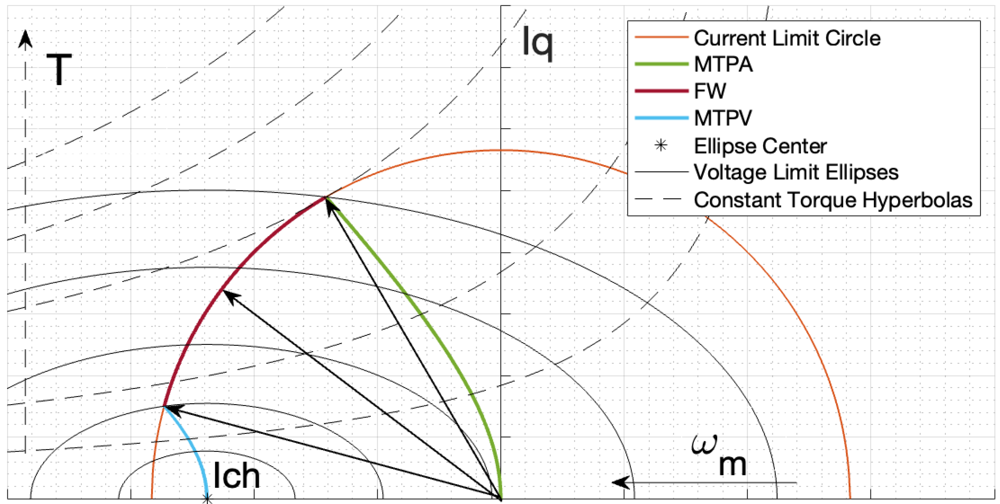
2. Operating Strategies in the Linear Model

Equation (1) reports the IPM machine voltage equations in the rotating d-q reference frame and synchronous with the rotor’s speed.

$${\overline{v}}_{dq}=R{\overline{i}}_{dq}+\frac{d}{dt}\left({\overline{\lambda }}_{dq}\right)+j{p}_p{\omega }_m{\overline{\lambda }}_{dq}$$

(1)

where:

• R: phase resistance;
• ${\overline{v}}_{dq}$: voltage vector;
• ${\overline{i}}_{dq}$: current vector;
• ${\omega }_m$: mechanical speed;
• $p_p$: pole pairs number;
• ${\overline{\lambda }}_{dq}={\overline{L}}_{dq}{\overline{i}}_{dq}+{\overline{\lambda }}_{pm,dq}$: flux linkage vector;
• ${\overline{\lambda }}_{pm,dq}=\left[\begin{array}{c}{\lambda }_{pm}\\ 0\end{array}\right]$: flux linkage due to PM;
• ${\overline{L}}_{dq}=\left[\begin{array}{cc}{L}_d& 0\\ 0& L_q\end{array}\right]$: inductance matrix.

Equation (1) can be split in two scalar equations for d and q axes as:

$$v_d=R{i}_d+L_d\frac{d}{dt}\left(i_d\right)-p_p{\omega }_m{L}_q{i}_q$$

(2)

$$v_q=R{i}_q+L_q\frac{d}{dt}\left(i_q\right)+p_p{\omega }_m\left(L_d{i}_d+{\lambda }_{pm}\right)$$

(3)

Neglecting the voltage drop across the resistance and considering steady-state operation, torque can be expressed as:

$$T=\frac{3}{2}{p}_p\left[{\lambda }_{pm}{i}_q+i_d{i}_q\left(L_d-L_q\right)\right]$$

(4)

The operating limits of the machine can be identified as curves in the d-q plane: the current limit is identified by a circle, Equation (5), and the voltage limit due to DC bus voltage can be expressed as in Equation (6).

$$i_d^2+i_q^2=I_{lim}^2$$

(5)

$$v_d^2+v_q^2=V_{lim}^2$$

(6)

In steady-state, the voltage limit can be represent with an ellipse in the d-q reference plane, Equation (7), by replacing Equations (2) and (3) in Equation (6) and neglecting the resistance drop.

$$\frac{{\left(I_d+\frac{{\lambda }_{pm}}{L_d}\right)}^2}{{\left(\frac{V_{lim}}{p_p{\omega }_m{L}_d}\right)}^2}+\frac{I_q^2}{{\left(\frac{V_{lim}}{p_p{\omega }_m{L}_q}\right)}^2}=1$$

(7)

where capital letters stand for stationary values.

The center of the ellipses is $[I_{ch};0]$, where $I_{ch}$ is referred to as the characteristic current of the machine that can be obtained with Equation (8).

$$I_{ch}=-\frac{{\lambda }_{pm}}{L_d}$$

(8)

The allowed operating region of the machine is defined by the intersection of the internal areas of the two curves of Equations (5) and (7), i.e., the Current Limit Circle (CLC) and the Voltage Limit Ellipses (VLE) of Figure 1.

It is useful to express steady-state components $I_d$ and $I_q$ as a function of the current space vector amplitude I and phase $\gamma$ as in Equation (9).

$$\left\{\begin{array}{c}{I}_d=Isin\gamma \\ I_q=Icos\gamma \end{array}\right.$$

(9)

By replacing Equation (9) in Equation (4), torque can be expressed as in (10).

$$T=\frac{3}{2}{p}_p\left[{\lambda }_{pm}Icos\gamma +I^{2}sin\gamma cos\gamma \left(L_d-L_q\right)\right]$$

(10)

In MTPA operations, the control acts to regulate the maximum torque for a fixed current amplitude. Considering Equation (10), MTPA locus can be expressed as Equation (11).

$$\begin{array}{c}\frac{d}{d\gamma }(T/I)=0\\ \\ \Rightarrow {\lambda }_{pm}sin\gamma +I(L_d-L_q)(si{n}^2\gamma -co{s}^2\gamma )=0\end{array}$$

(11)

The locus stated by Equation (11) is based on a number of assumptions:

• Pure sinusoidal currents and air gap magnetic field distribution;
• No cross-coupling between the equivalent magnetic circuit and the d-q axes. The two axes are magnetically decoupled because they are at 90 electrical degrees;
• No saturation effects, i.e., no variation of the inductances versus currents.

These assumptions are too restrictive for a complete model of an IPM machine, especially the last one. In fact, a machine’s inductances values cannot be considered constant, but they vary as a function of both current vector amplitude and phase: $L_d(I,\gamma )$ and $L_q(I,\gamma )$.

Therefore, the computation of the torque Equation (11) should include the partial derivative of the inductances:

$${\lambda }_{pm}sin\gamma +I\left[\frac{\delta L_d(I,\gamma )}{\delta \gamma }-\frac{\delta L_q(I,\gamma )}{\delta \gamma }\right](si{n}^2\gamma -co{s}^2\gamma )=0$$

(12)

By taking into account the variation of the inductances with the operating point, it is not possible to obtain a simple analytical expression for the MTPA locus as in the previous linear model case. In addition to that, the functions $L_d(I,\gamma )$ and $L_q(I,\gamma )$ should be estimated starting from a complete map of the equivalent inductances over all the possible operating points of the machine. Similar issues occur in the computation of the other two operating modes loci: FW and MTPV.

The maximum-torque operating point lies on the intersection between the CLC and the MTPA loci, but for high speeds, also the VLE must be taken into account. In fact, MTPA operation is possible only below a certain speed referred to as base speed. Above the base speed, the shrinkage of the VLE causes the maximum-torque point to lie outside voltage limit, making the operating point inaccessible for steady-state operations (Figure 1). For each operating point of MTPA $(I_d;I_q)$, the base speed value can be computed as the intersection between MTPA (Equation (11)) and the VLE Equation (7)).

$${\omega }_{base}=\frac{V_{lim}}{p_p\sqrt{{(L_d{I}_d+{\lambda }_{pm})}^2+{\left(L_q{I}_q\right)}^2}}$$

(13)

As a consequence, when higher speeds are required, the machine must be operated in FW mode, where the maximum output torque decreases with speed. The terminal voltage and the amplitude of the current vector are kept constant at their limits $V_{lim}$ and $I_{lim}$, while the phase angle is increased with the speed, thanks to the demagnetizing d-axis reaction. This trajectory can be expressed as the intersection between the CLC (Equation (5)) and the VLE (Equation (7)) as shown in (14).

$$\begin{array}{c}\left\{\begin{array}{c}{I}_d^2+I_q^2=I_{lim}^2\\ \frac{{\left(I_d+\frac{{\lambda }_{pm}}{L_d}\right)}^2}{{\left(\frac{V_{lim}}{p_p{\omega }_m{L}_d}\right)}^2}+\frac{I_q^2}{{\left(\frac{V_{lim}}{p_p{\omega }_m{L}_q}\right)}^2}=1\end{array}\right.\\ \\ \Rightarrow I_d=\frac{L_d{\lambda }_{pm}}{L_d^2-L_q^2}\left\{-1+\sqrt{1-\frac{L_d^2-L_q^2}{L_d{\lambda }_{pm}^2}\left[{\lambda }_{pm}^2+L_q^2{I}_{lim}^2-{\frac{V_{lim}}{p_p{\omega }_m}}^2\right]}\right\}\end{array}$$

(14)

In order to take into account nonlinearities in the computation of FW strategy, the constant inductances of Equation (14) should be replaced with $L_d(I,\gamma )$ and $L_q(I,\gamma )$. However, this is far too complex for a real-time implementation.

It is not possible to operate up to an arbitrarily high velocity in FW operation, but there is an FW speed limit. The maximum achievable speed corresponds to the smallest VLE touching the CLC, that can be computed from Equation (7) with $I_q=0$ and $I_d=-I_{lim}$.

$${\omega }_{FW,end}=\frac{V_{lim}}{p_p(L_d{I}_{lim}+{\lambda }_{pm})}$$

(15)

However, if the characteristic current of the machine falls inside the CLC, it is possible to reach a high speed with MTPV operation. In this case, the optimal current vector follows the MTPV trajectory up the point $[I_{ch};0]$, corresponding to infinite speed and zero torque operation. In MTPV, the voltage is not sufficient to hold current to $I_{lim}$ and the flux linkage $\lambda$ must be decreased with the increase of speed, as $\lambda \approx V_{lim}/p_p{w}_m$. Actually, MTPV operation comes into action at the intersection point between its trajectory and the CLC (Figure 1). In fact, from that point, it is possible to obtain the same torque output for a lower current amplitude.

The computation of MTPV trajectory is easier in a new D-Q reference frame, whose origin is in the centre of the VLE. So doing, the current components become as in Equation (16).

$$\left\{\begin{array}{c}{I}_D=\frac{{\lambda }_{pm}+L_d{I}_d}{L_q}\\ I_Q=I_q\end{array}\right.$$

(16)

By replacing Equation (16) in Equation (7), the VLE becomes a voltage limit circle as shown in Equation (17).

$$\frac{I_D^2}{{\left(\frac{V_{lim}}{p_p{\omega }_m{L}_q}\right)}^2}+\frac{I_Q^2}{{\left(\frac{V_{lim}}{p_p{\omega }_m{L}_q}\right)}^2}=1$$

(17)

The new current vector in D-Q reference frame can be defined in terms of amplitude and phase as in Equation (18).

$$\left\{\begin{array}{c}{I}^{\prime }=\sqrt{I_D^2+I_Q^2}=\frac{V_{lim}}{p_p{\omega }_m{L}_q}\\ {\gamma }^{\prime }={tan}^{-1}\left(\frac{I_D}{I_Q}\right)\end{array}\right.$$

(18)

By replacing Equation (18) into Equation (4):

$$T=\frac{3}{2}\frac{V_{lim}}{{\omega }_m{L}_q}\left[\frac{V_{lim}}{p_p{\omega }_m}\left(1-\frac{Lq}{Ld}\right)sin{\gamma }^{\prime }cos{\gamma }^{\prime }+{\lambda }_{pm}\frac{Lq}{Ld}cos{\gamma }^{\prime }\right]$$

(19)

The MTPV locus can be obtained from torque Equation (19) with respect to the current angle in the D-Q frame:

$$\begin{array}{c}\frac{d}{d{\gamma }^{\prime }}(T/V_{lim})=0\\ \\ \Rightarrow (L_d-L_q)\left[{\left(\frac{L_d{I}_d+{\lambda }_{pm}}{L_q}\right)}^2-I_q^2\right]+{\lambda }_{pm}\left(\frac{L_d{I}_d+{\lambda }_{pm}}{L_q}\right)=0\end{array}$$

(20)

As for MTPA, Equation (20) is based on restrictive assumptions, thus more accurate results can be achieved only including partial derivative of inductances.

In conclusion, a closed analytical formulation is possible if and only if the behavior of inductances is known as a function of the current amplitude and phase angle. Moreover, this would result in a very complex solution, not suited to real-time implementation.

This paper proposes a viable solution taking into account the variation of $L_d$ and $L_q$ with the working point of the reference machine. Complete maps of the two equivalent inductances along the d-q axes are defined thanks to 2-D FEA. Then, the computation of MTPA, FW and MTPV curves follows an algorithmic approach, based on the above mentioned maps.

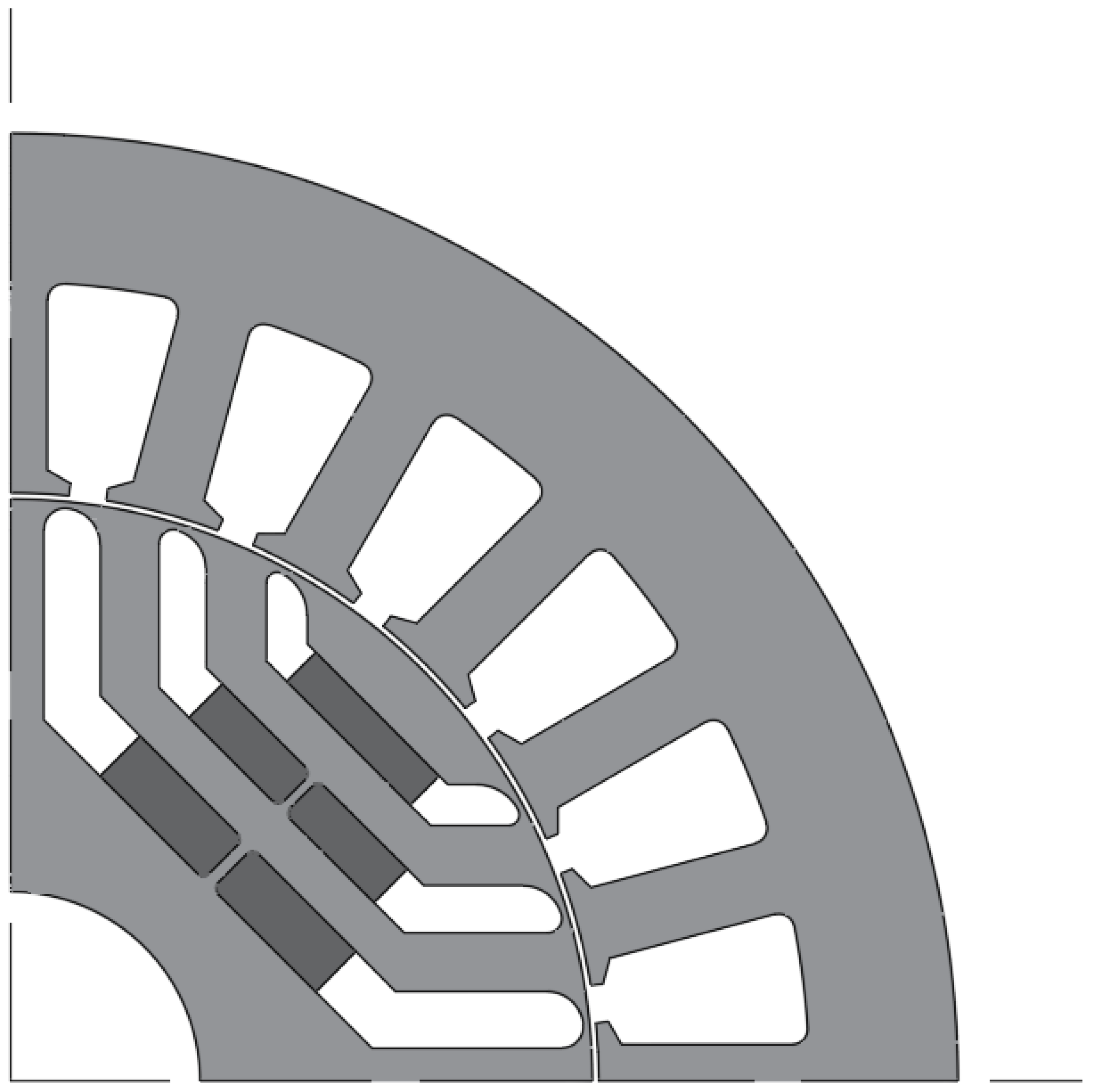
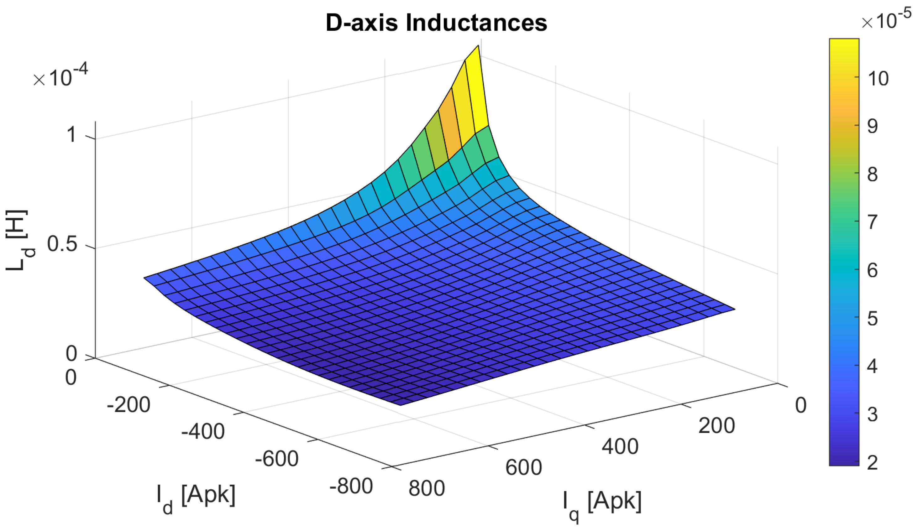
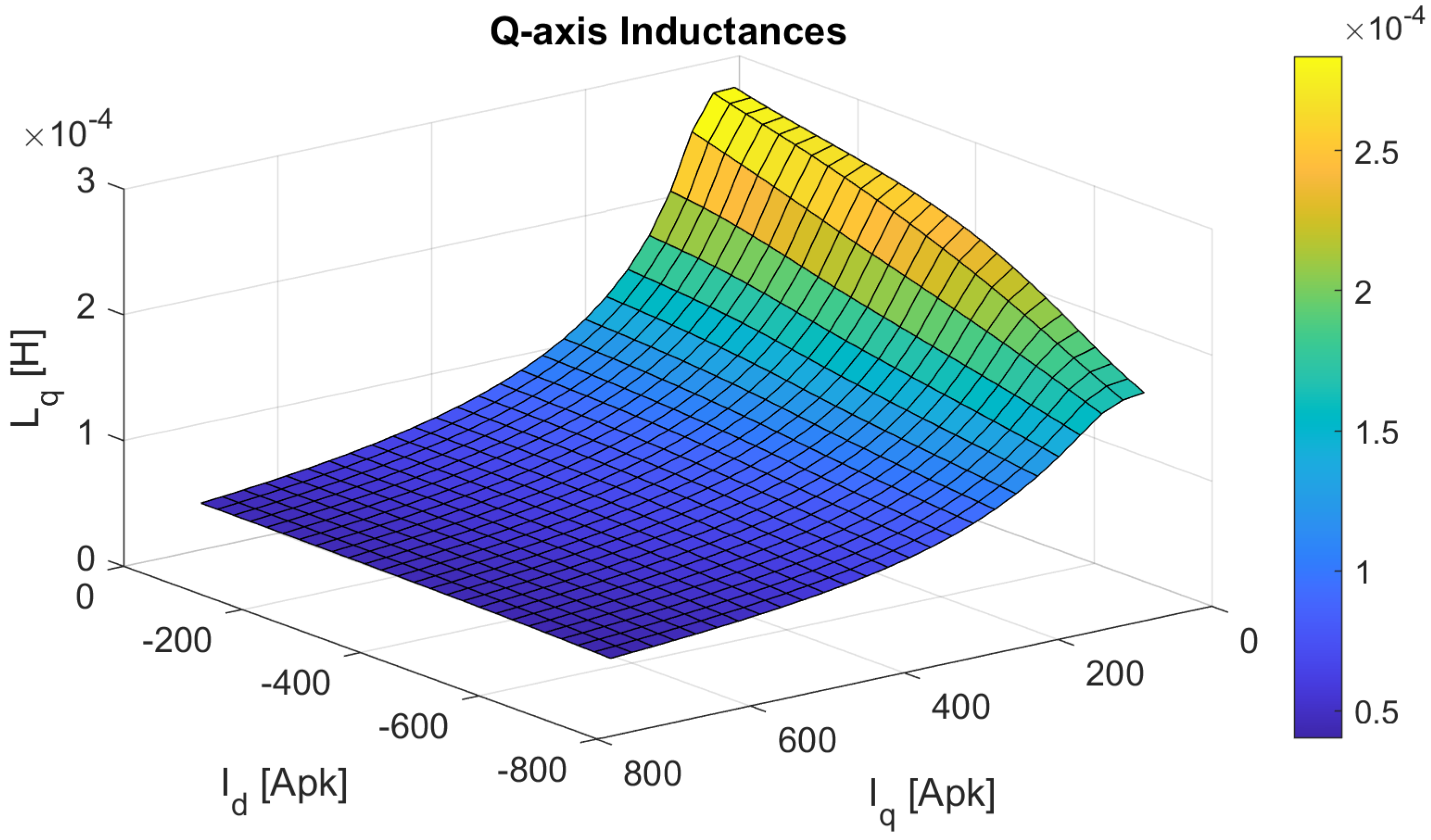
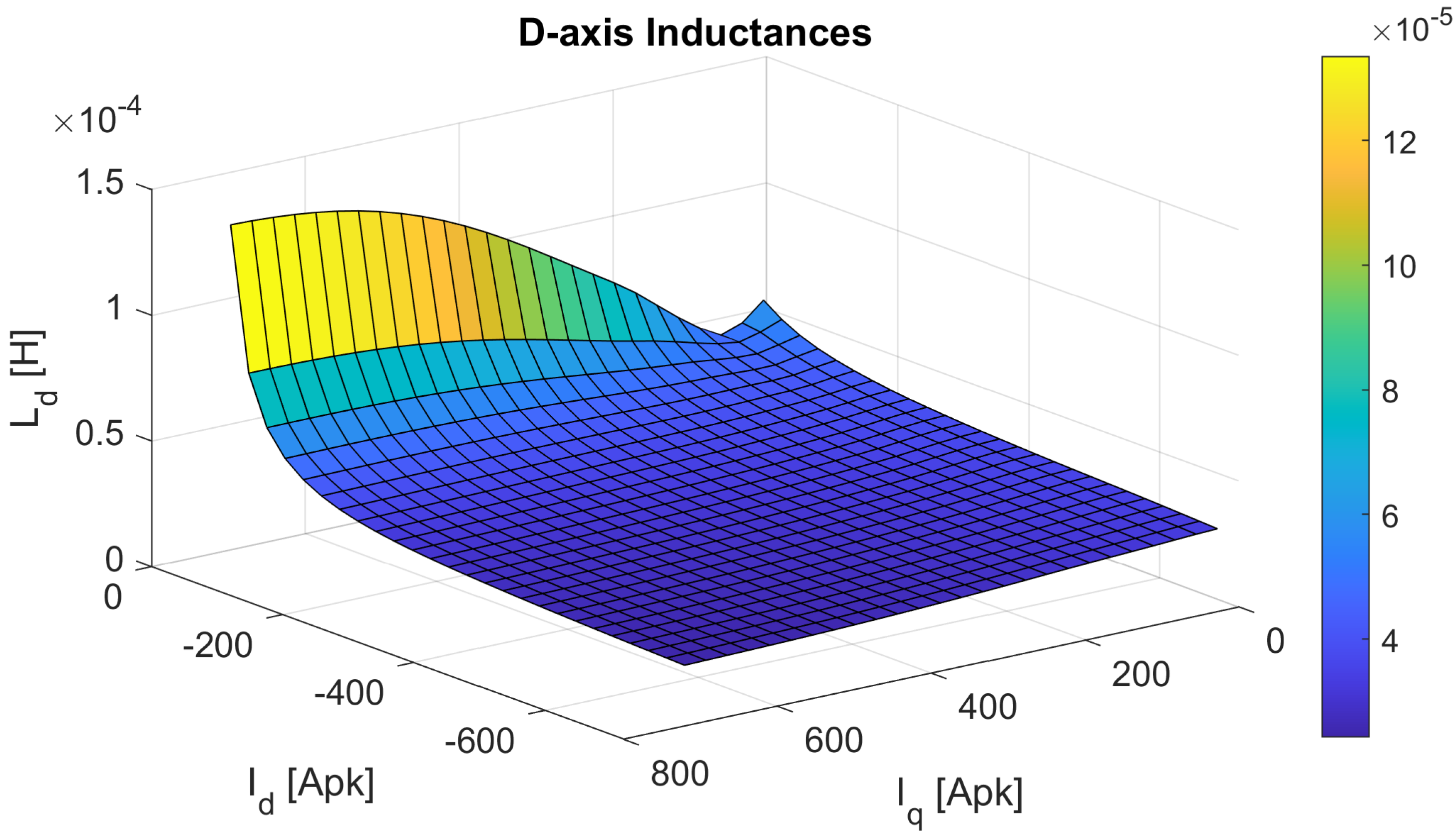
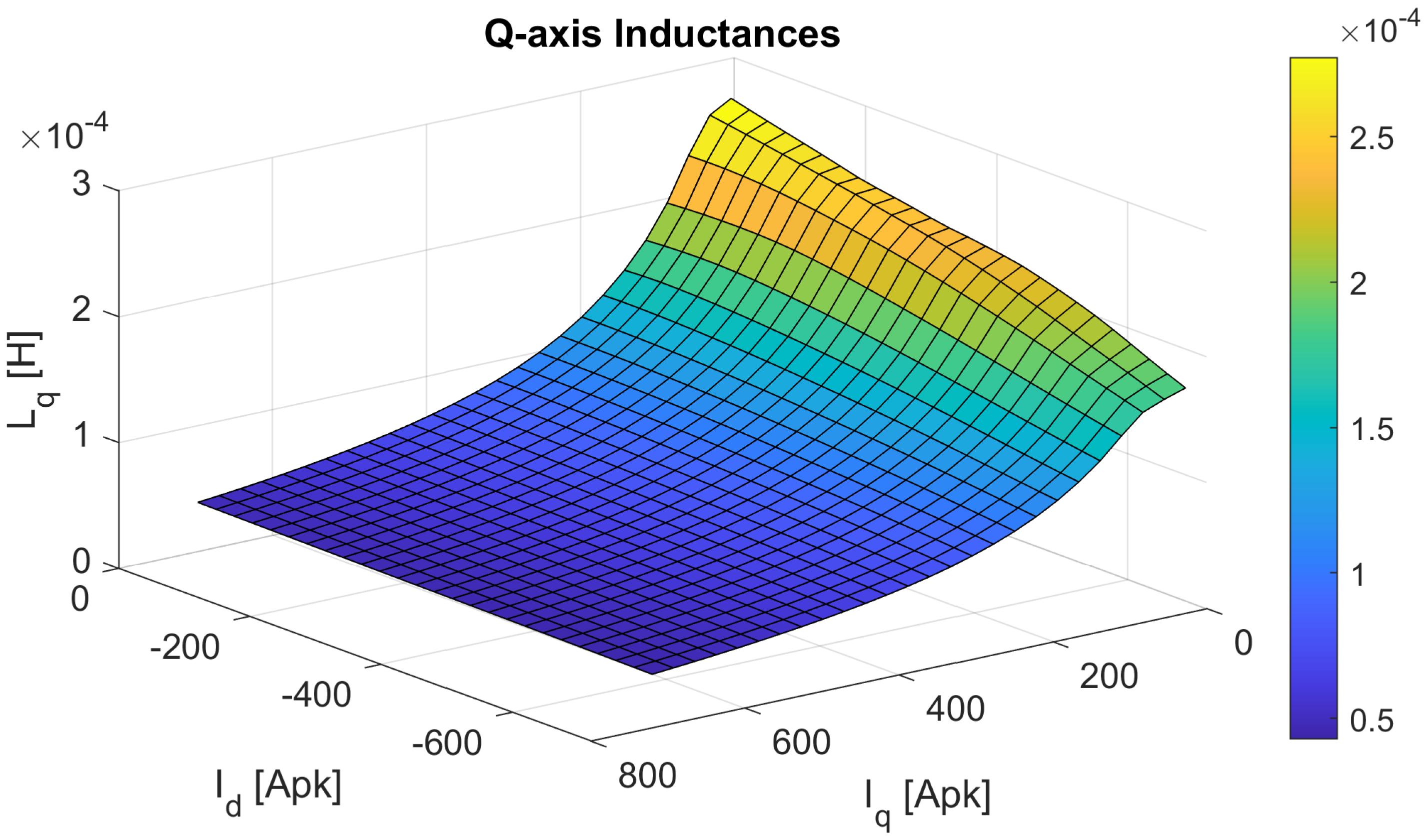
3. Finite Element Analysis for Magnetic Model Mapping

This section briefly describes the two different 2-D FEA methods employed to model the nonlinear magnetic behaviour of the reference IPM machine. The geometry of the chosen reference machine is shown in Figure 2 and its parameters are listed in Table 1.

3.1. Standard Method

The first adopted method (Standard Method) is based on standard nonlinear magnetostatic simulations. Specifically, it uses only one nonlinear magnetic 2-D FEA, that includes both armature current and permanent-magnets as MMF sources. FEA simulations were performed with different values of the stator currents in order to obtain a complete map of the $L_d$ and $L_q$ inductances in the d-q plane.

The inductances maps for the reference machine are shown in Figure 3 and Figure 4.

3.2. Frozen Permeability Method

The Frozen Permeability method (FP) relies on two different sets of simulations. The first simulation is run in a specific operating point, generally rated operation, and the nonlinear magnetic model is obtained via 2-D FEA considering MMF contributions from armature currents and permanent-magnets. Then, the iron permeability is computed and stored for each mesh element by this nonlinear magnetic field analysis. Finally, permeability values are set for a second linear 2-D FEA simulation where permanent-magnets’ MMF is set to zero.

Thanks to FP the stator inductances are evaluated with the actual working point of the ferromagnetic material. Hence, the estimation of inductances is accurate even when the permanent-magnets’ MMF is set to zero, since FP includes the effects of permanent-magnets in the working point of stator and rotor laminations on the $B-H$ curve Further details on FP method can be retrieved in [35,36]. This method provides inductance values significantly different from the Standard Method.

Like the Standard Method, the complete maps of $L_d$ and $L_q$ inductances are obtained by a set of simulations with different couples of $i_d-i_q$ currents. The maps of the magnetic model of reference machine are shown in Figure 5 and Figure 6.

4. Nonlinear d-q Model Computation

In the following, the algorithms developed for each control trajectory will be presented. The code is based on the $L_d$ and $L_q$ maps obtained from the nonlinear magnetic models computed by the two presented 2-D FEA methods. Before introducing control strategies algorithms, two control loops must be presented: iterative numeric process and stationary loop.

The iterative numeric process is necessary to overcome an existing circular dependency: in order to compute the operating point $(I_d;I_q)$, the values of $L_d$ and $L_q$ must be known; however, these values are functions of the still unknown $(I_d;I_q)$ values. The iterative numeric process is adopted for all the curves and operates as follows:

• Define a starting value of $L_d$, $L_q$ considering a known point belonging to the desired control curve;
• Compute $I_d$, $I_q$ according to Equation (11), Equation (14) or Equation (20) for MTPA, FW and MTPV respectively;
• Re-compute $L_d$, $L_q$ with the current values of $I_d$, $I_q$ and the inductances map;
• Use the new value of $L_d$, $L_q$ computed in the previous bullet for the next iteration.

This iterative process can be further improved by a stabilizing loop that reiterates the previous procedure until the difference between the current value and the previous one is below a fixed threshold. As an example, this method was used for the estimation of the characteristic current $I_{ch}$, that has a circular dependency on $L_d$:

• $I_{ch}$ is estimated with Equation (8) using the mean value of $L_d$ on the overall domain;
• $L_d$ and $L_q$ are computed in the point $(I_{ch};0)$ with the inductances map;
• $I_{ch}$ is re-computed with Equation (8);
• The difference $\Delta I_{ch}$ between the current $I_{ch}$ value and the previous one is computed and compared with a desired threshold.

This loop continues iterating until $\Delta I_{ch}$ decreases below the fixed threshold. In this way, undesired numerical oscillations are limited and $L_d$ and $L_q$ converge to the most precise values in the point of interest.

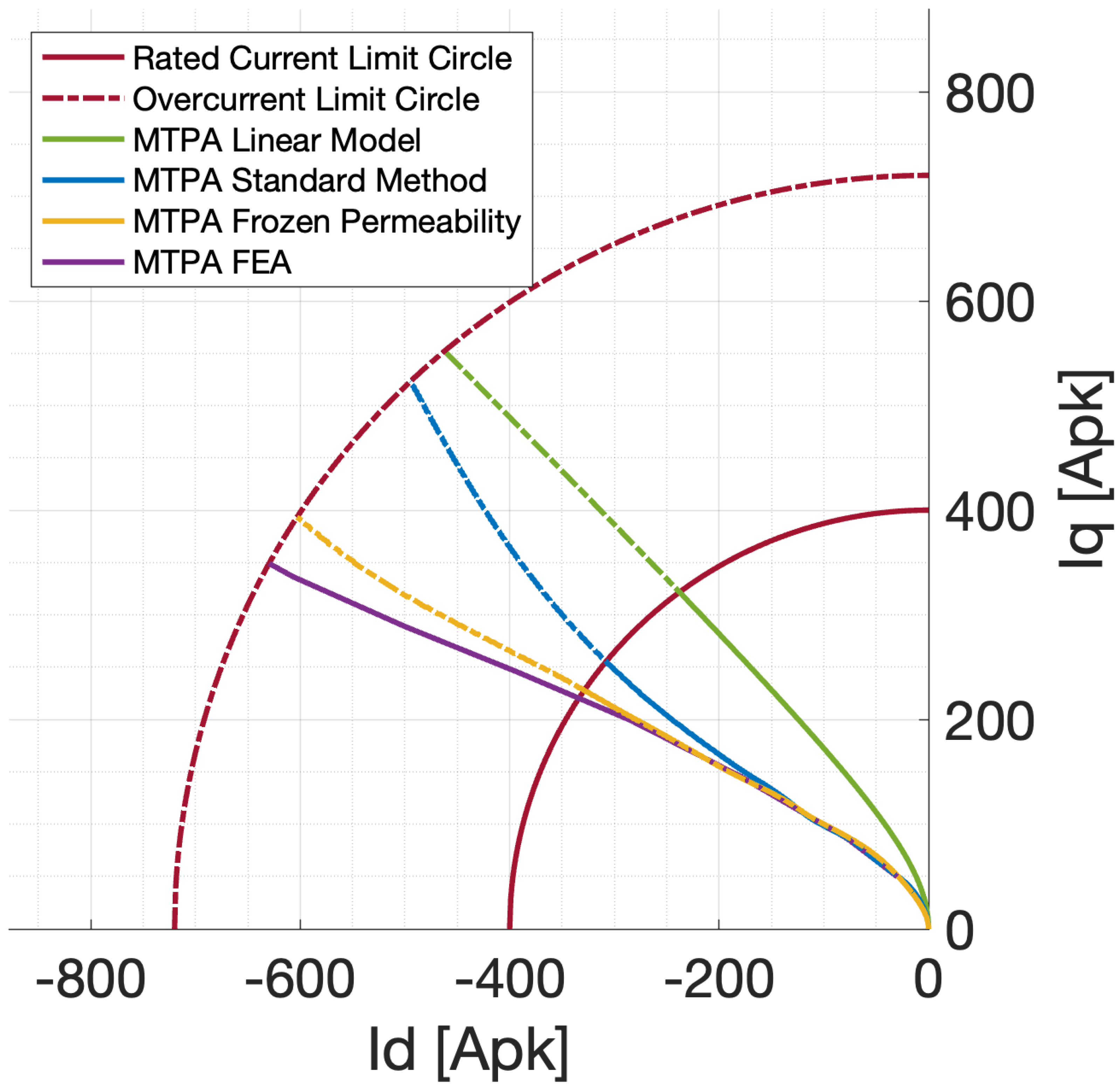
4.1. Maximum Torque Per Ampere (MTPA)

As shown in Section 2, MTPA curve cannot be expressed in a closed-form, when numerical maps of $L_d$ and $L_q$ are used. The numeric algorithm developed for MTPA iterates as follows:

• A space vector of current amplitude $\left[I\right]$ is defined ranging from 0 to current limit $I_{lim}$ value;
• For each value of $\left[I\right]$, a vector of current phase $\left[\gamma \right]]$ is defined ranging from 90° to 180°;
• Each couple of the matrix $[I;\gamma ]$ identifies an operating point in the second quadrant of the d-q plane;
• For each couple, $L_d$ and $L_q$ are interpolated from inductances maps at disposal. Torque is computed by Equation (4) and stored in a matrix;
• For each value of $\left[I\right]$, the maximum torque is computed comparing the matrix elements corresponding to each value of $\left[\gamma \right]$. Also the corresponding values of $L_d$, $L_q$, $I_d$ and $I_q$ are computed and stored.

In this way, the MTPA trajectory is identified and the base speed vector ${\omega }_{base}$ can be computed with Equation (13) for each value of $\left[I\right]$. The ending element of ${\omega }_{base}$ vector will be used for the computation of FW trajectory.

4.2. Flux Weakening (FW)

While MTPA points are computed starting from a $[I;\gamma ]$ matrix, FW and MTPV points are based on a speed vectors. In fact, these last two strategies come into play for high speeds, and the maximum output torque is fixed by the speed. Hence, the procedure for FW computation is similar to the one for MTPA, but based on a speed vector. The FW algorithms works as follows:

• The last element of the base speed vector $\left[{\omega }_{base}\right]$ of MTPA is selected as the starting element for the FW speed (${\omega }_{FW,start}$);
• The limit speed in FW (${\omega }_{FW,end}$) is computed according to Equation (15);
• The FW speed vector ranges from ${\omega }_{start}$ to ${\omega }_{lim}$;
• Starting values of $L_d$ and $L_q$ are computed in the end point of MTPA trajectory: $L_d=L_d(I_{d_{end,MTPA}},I_{q_{end,MTPA}})$ and $L_q=L_q(I_{d_{end,MTPA}},I_{q_{end,MTPA}})$;
• For each element of the speed vector, the following parameters are computed and stored:

  -

  $I_d$ by Equation (14);

  -

  $I_q$ by the Current Limit Circle of Equation (5);

  -

  Torque by Equation (4);

  -

  The new values of $L_d$ and $L_q$ to be used for the next speed value are interpolated from the map with the current $I_d$ and $I_q$ values.

A graphical representation of the procedure is depicted in Figure 7.

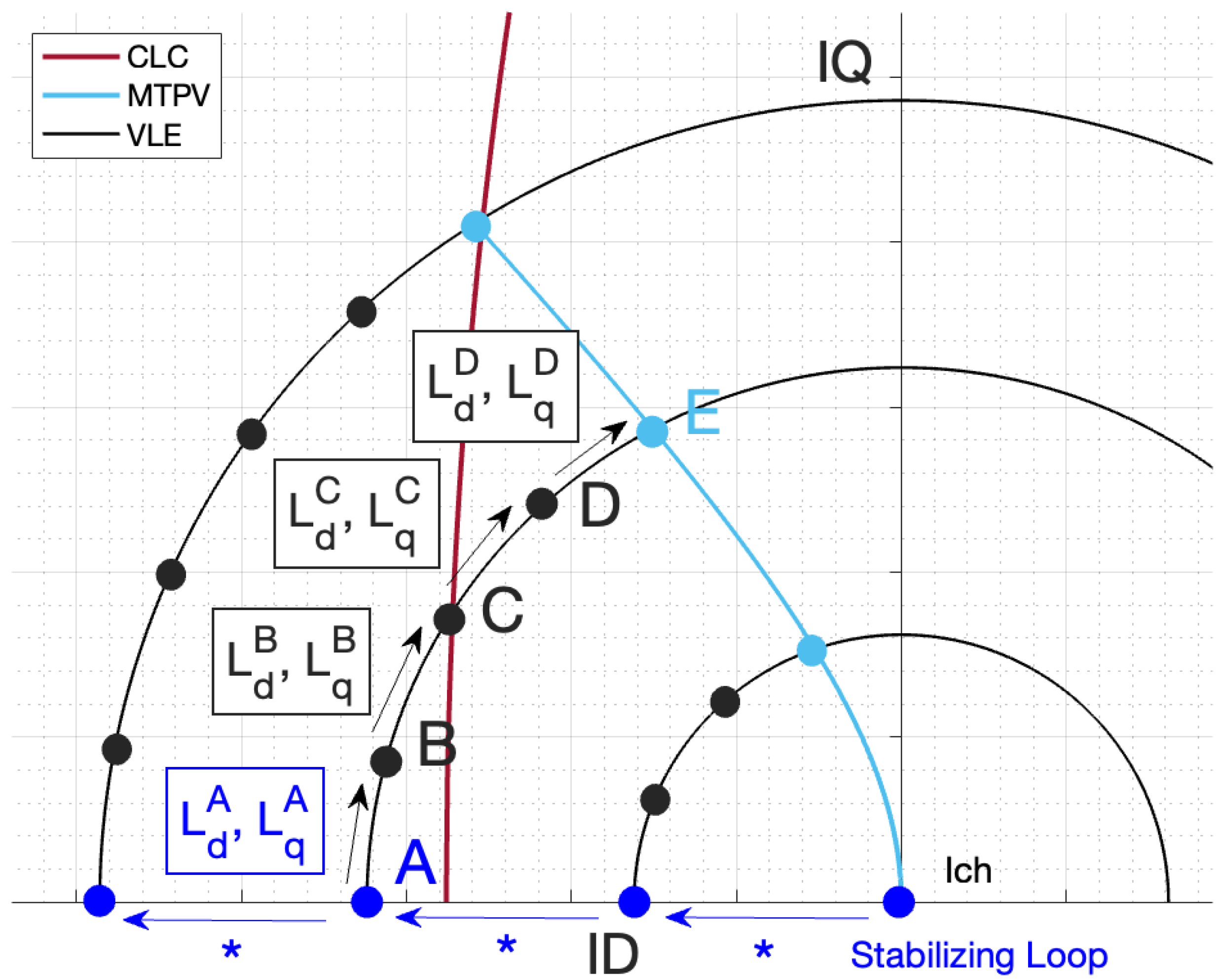
4.3. Maximum Torque Per Volt (MTPV)

The algorithm for MTPV starts from a speed vector, considering $I_q=0$ and then iterating for the overall range of $\gamma$. This procedure is more complex than the previous ones: in MTPA the computation was based on a $[I;\gamma ]$ matrix and in FW a starting point was available, being the ending point of MTPA. Here, the starting values of $L_d$, $L_q$ and $\gamma$ are required at the beginning of each iteration. Hence, the point $(I_{ch};0)$ is chosen as the starting point for the trajectory computation, that corresponds to the infinite velocity point. In order to practically define a speed vector, the infinite velocity has been approximated with a very high velocity. Thus, the starting point of MTPV is located at $\gamma$ = 180° and an high speed value. Specifically, the algorithm for MTPV is based on the following loop:

• Starting values of $L_d$ and $L_q$ are computed in the starting point $(I_{ch};0)$ with the stabilizing loop described in Section 4;
• For each element of the speed vector with ${\gamma }^{\prime }=180°$, the $L_d$ and $L_q$ values computed at the previous iteration are taken as starting values and the stabilizing loop is performed. After their values are fixed with high accuracy, the following parameters are computed:

  -

  $I^{\prime }$ and the $I_D$ are computed by Equation (18) where $I_Q=0$;

  -

  $I_d$ and $I_q$ are computed by Equation (16);

  -

  Torque is computed by Equation (4) and stored in a matrix;

  -

  The new values of $L_d$ and $L_q$ to be used for the next speed value are interpolated from the map with the current $I_d$ and $I_q$ values.

So doing, the inductances and the torque on the d-axis have been fixed. Starting from these values, it is possible to iterate the procedure on the overall range of ${\gamma }^{\prime }$. For each speed value:

• $I^{\prime }$ is computed by Equation (18);
• $I_D$ and $I_Q$ are computed from $I^{\prime }$ and ${\gamma }^{\prime }$ by Equation (18);
• $I_d$ and $I_q$ are computed by Equation (16);
• Torque is computed by Equation (4) and stored in a matrix;
• The new values of $L_d$ and $L_q$ to be used for the next ${\gamma }^{\prime }$ value are interpolated from the map with the current $I_d$ and $I_q$ values.

Once the complete torque matrix is computed for each operating point of $[{\omega }_{MTVP},\gamma ]$ the maximum torque is computed comparing the matrix elements corresponding to each value of $\left[\gamma \right]$. Also the corresponding values of $L_d$, $L_q$, $I_d$ and $I_q$ are computed and stored. In this way, the operating points of MTPV trajectory are obtained.

A graphical representation of the procedure is depicted in Figure 8.

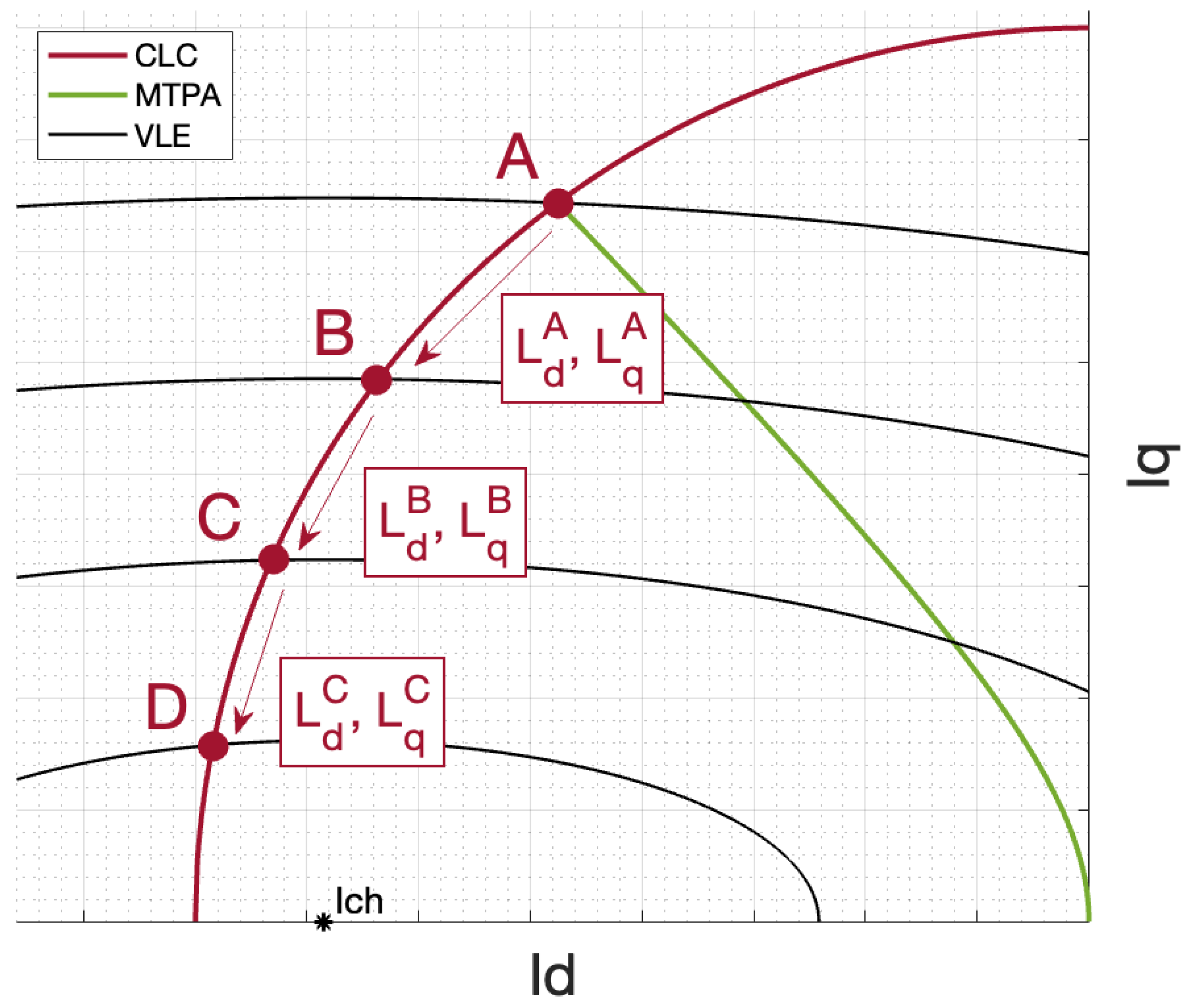
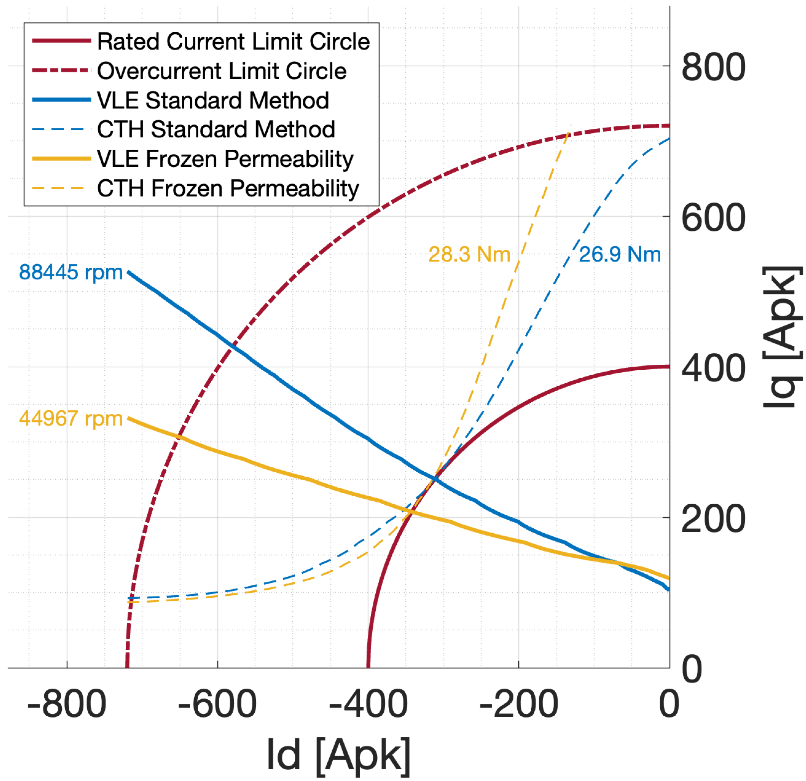
4.4. Voltage Limit Ellipses

As for the previous curves, also for the Voltage Limit Ellipses, the initial values for $L_d$ and $L_q$ must be set. For each ellipse, a initial point was chosen on the MTPA trajectory, computed in the previous subsection. Then, the points of the ellipse were computed iterating for lower $I_d$ values (moving to the left) and higher $I_d$ values (moving to the right)—i.e., d-axis current is negative. Hence, the ellipse is divided in a left and right side with respect to the MTPA curve. In the following, only the algorithm approach for left part of VLE is described.

A set of values $\left[I_q\right]$ for which the corresponding ellipses will be evaluated is defined and for each element of this vector, then the following steps are carried out:

• The corresponding $I_d$ on the MTPA trajectory is identified;
• The starting values of $L_d$ and $L_q$ are interpolated from the inductance map;
• The corresponding speed value is computed by Equation (7);
• A vector ranging from the identified $I_d$ to the current limit $-I_{lim}$ is defined. For each value of this vector:

  -

  $I_q$ is evaluated with the $L_d$ and $L_q$ of the previous step by Equation (7);

  -

  The new $L_d$ and $L_q$ with the current values of $I_d$ and $I_q$ are interpolated from the maps for the next iteration.

As an example, if the ending point of MTPA is used for the computation, the voltage limit ellipse corresponding to the rated speed will be obtained. The code for the right part of the ellipse is similar to the left part one, but the vector of $I_d$ values ranges up to $I_{lim}$ instead of $-I_{lim}$.

4.5. Constant Torque Hyperbolas

The Constant Torque Hyperbolas are computed with the same method of the Voltage Limit Ellipses and, in the following, only the code of left part is described. A set of values $\left[I_q\right]$ for which the corresponding hyperbole will be evaluated is defined and for each element of this vector, the following steps are carried out:

• The corresponding $I_d$ on the MTPA trajectory is identified;
• The starting values of $L_d$ and $L_q$ are interpolated from the inductance map;
• The corresponding torque value is computed by Equation (4);
• A vector ranging from the identified $I_d$ to the current limit $-I_{lim}$ is defined. For each value of this vector:

  -

  $I_q$ is evaluated with the $L_d$ and $L_q$ of the previous step by Equation (4);

  -

  The new $L_d$ and $L_q$ with the current values of $I_d$ and $I_q$ are interpolated from the map for the next iteration.

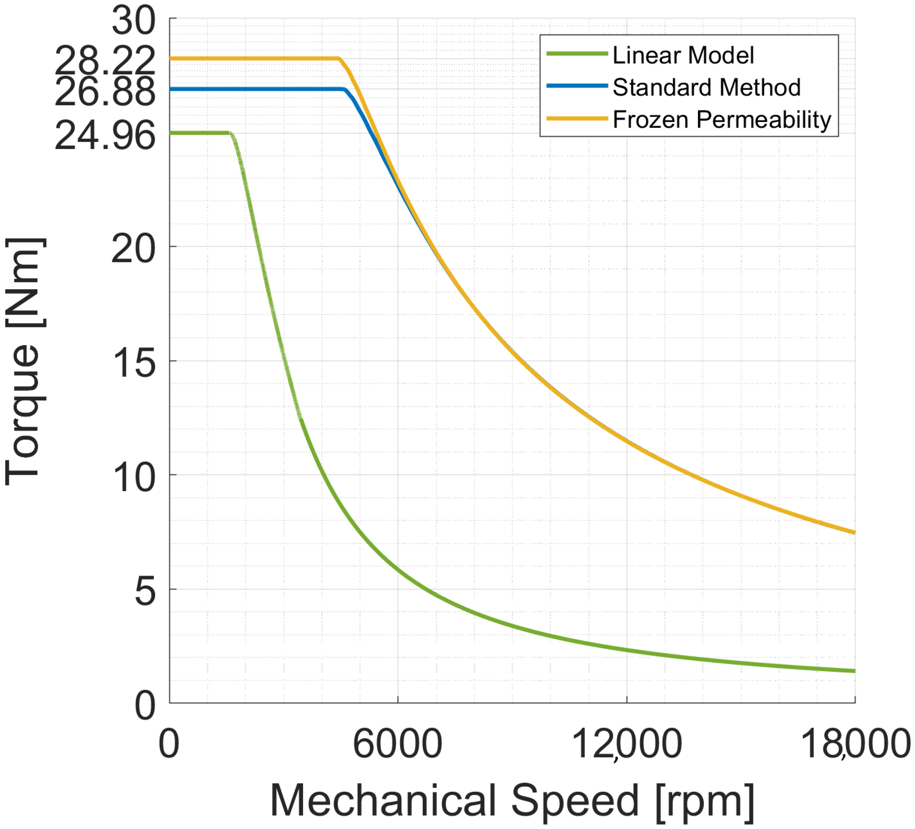
5. Results and Comparisons

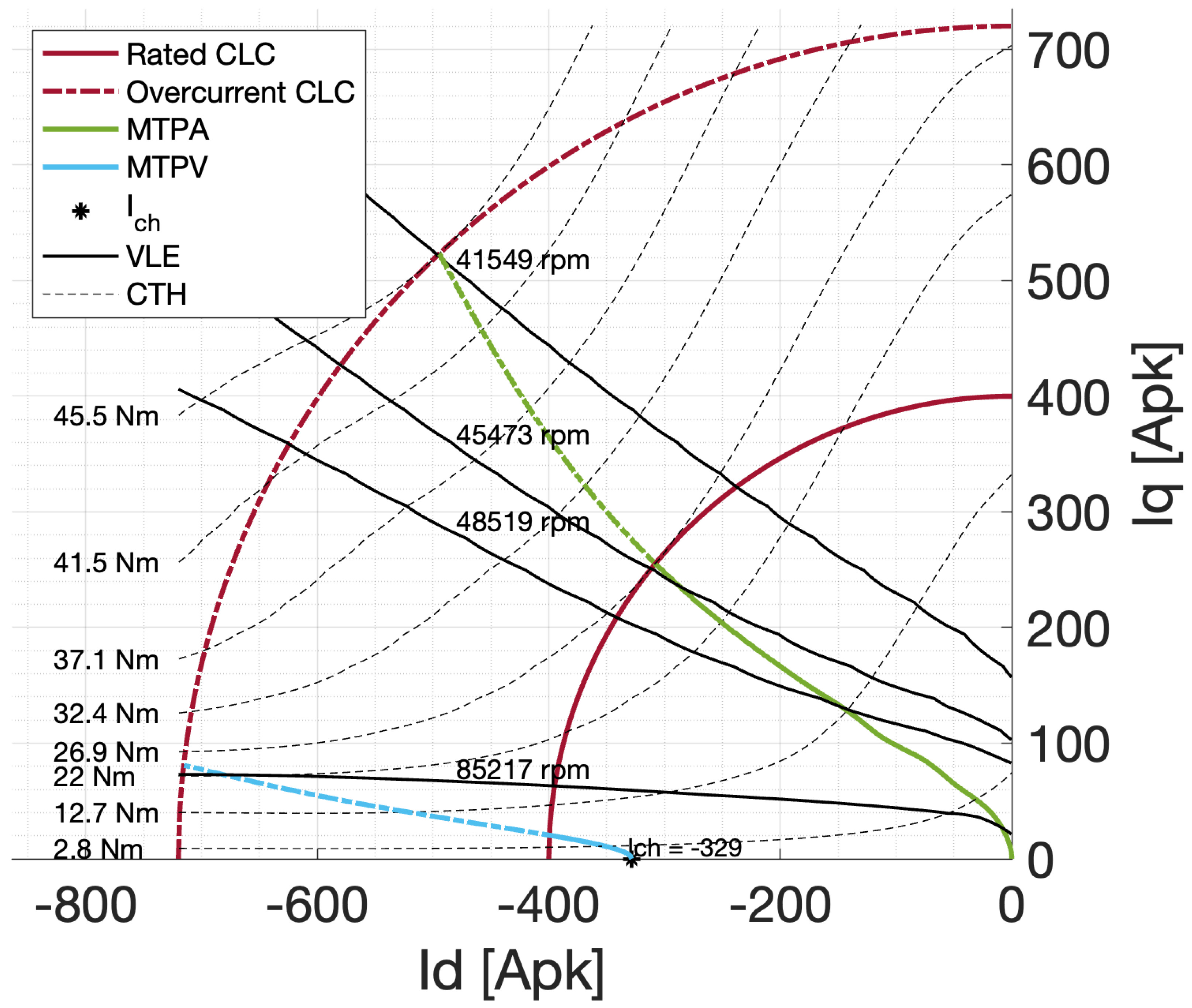
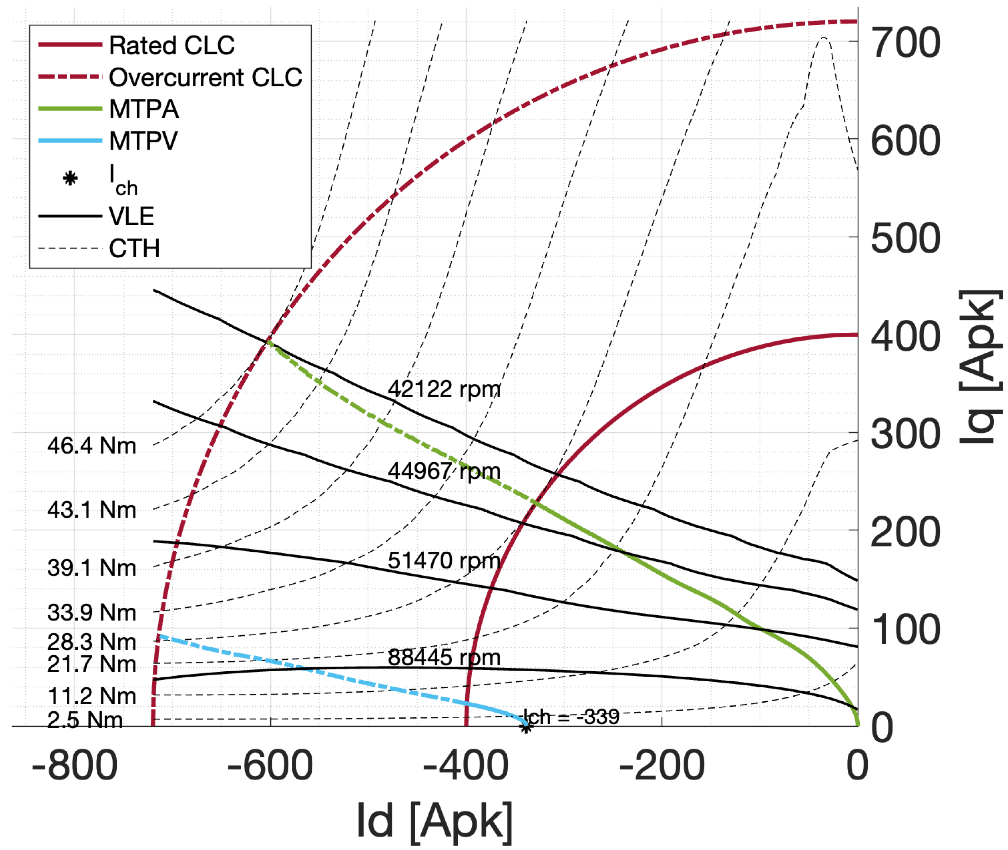
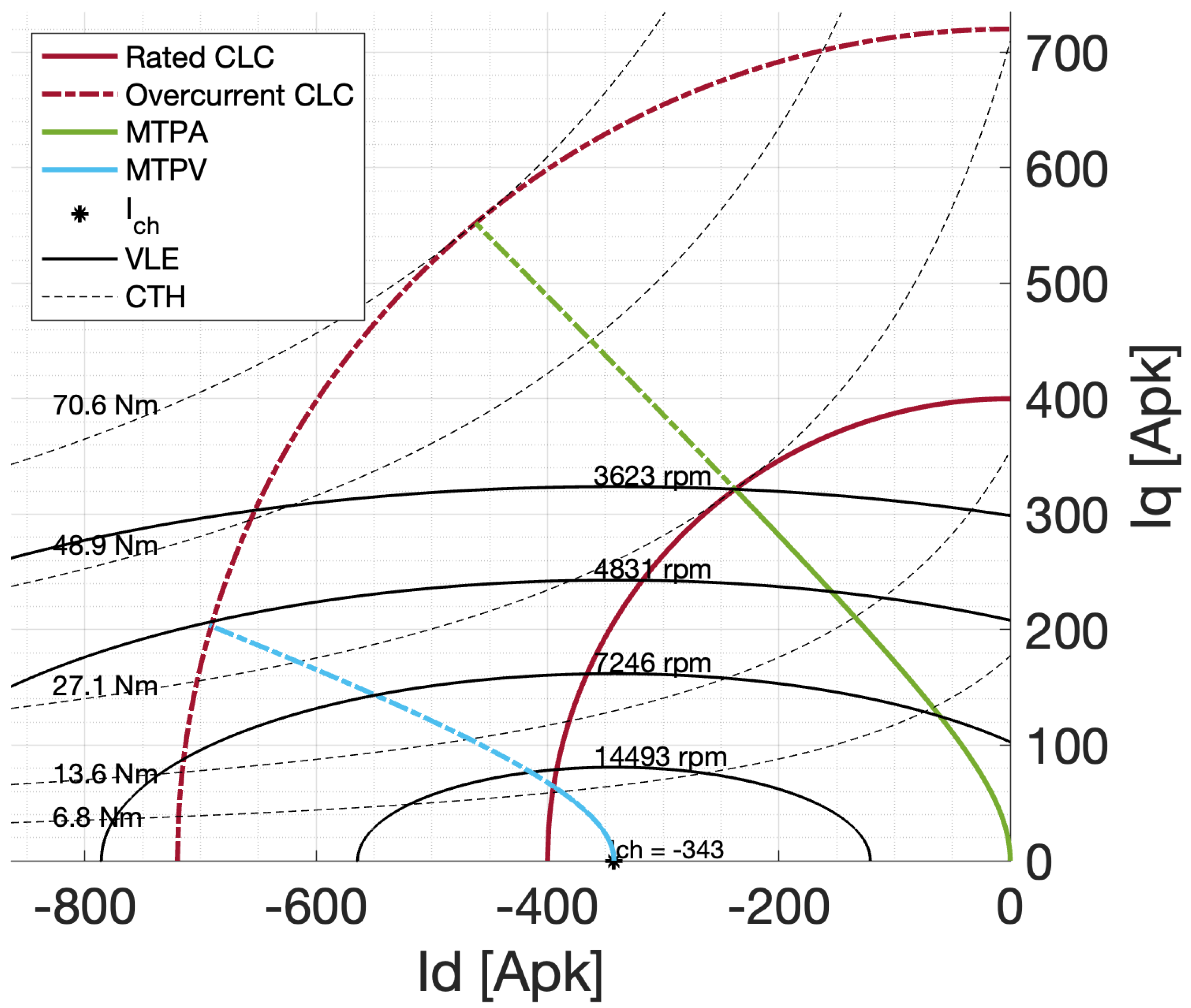
5.1. Generated Control Trajectories

The control trajectories on the d-q plane were computed with both Standard Method and FP. The results are reported in Figure 9 and Figure 10 along with the curves obtained with the conventional linear magnetic model (Figure 11) in order to provide a clear comparison about their performance.

In the pictures, MTPA curves are drawn both in rated current case (solid line) and in overcurrent case (dashed line). MTPA trajectory is remarkably different with the three methods, especially at high currents (dashed line). In fact due to high saturation, inductances computed with FP differ significantly from the ones computed with the Standard and the linear method.

The Voltage Limit Ellipses (black solid lines) are very different from the ideal ellipses of the conventional linear model (where the $L_d$ and $L_q$ are assumed to be constant). Specifically, on the left side of the d-q plane the ellipses moves away from the d-axis. Similarly to the case of MTPA, the linear model is less accurate when the amplitude of the current vector increases. These phenomena cause differences in the MTPA base speed and FW limit speed. On the other hand, the characteristic current point $[I_{ch};0]$ is similar for both the approaches, falling inside the rated current limit circle.

MTPA and MTPV curves are reported in the same figure for FP and Standard Method (Figure 12): MTPA trajectory computed with FP is more tilted towards the negative d-axis, underlining a better capability of such method to detect the correct behaviour of the machine when saturation starts to be non-negligible.

Figure 13 highlights the differences between the two methods for the Voltage Limit Ellipse (computed at base speed) and the Constant Torque Hyperbola (computed at rated torque).

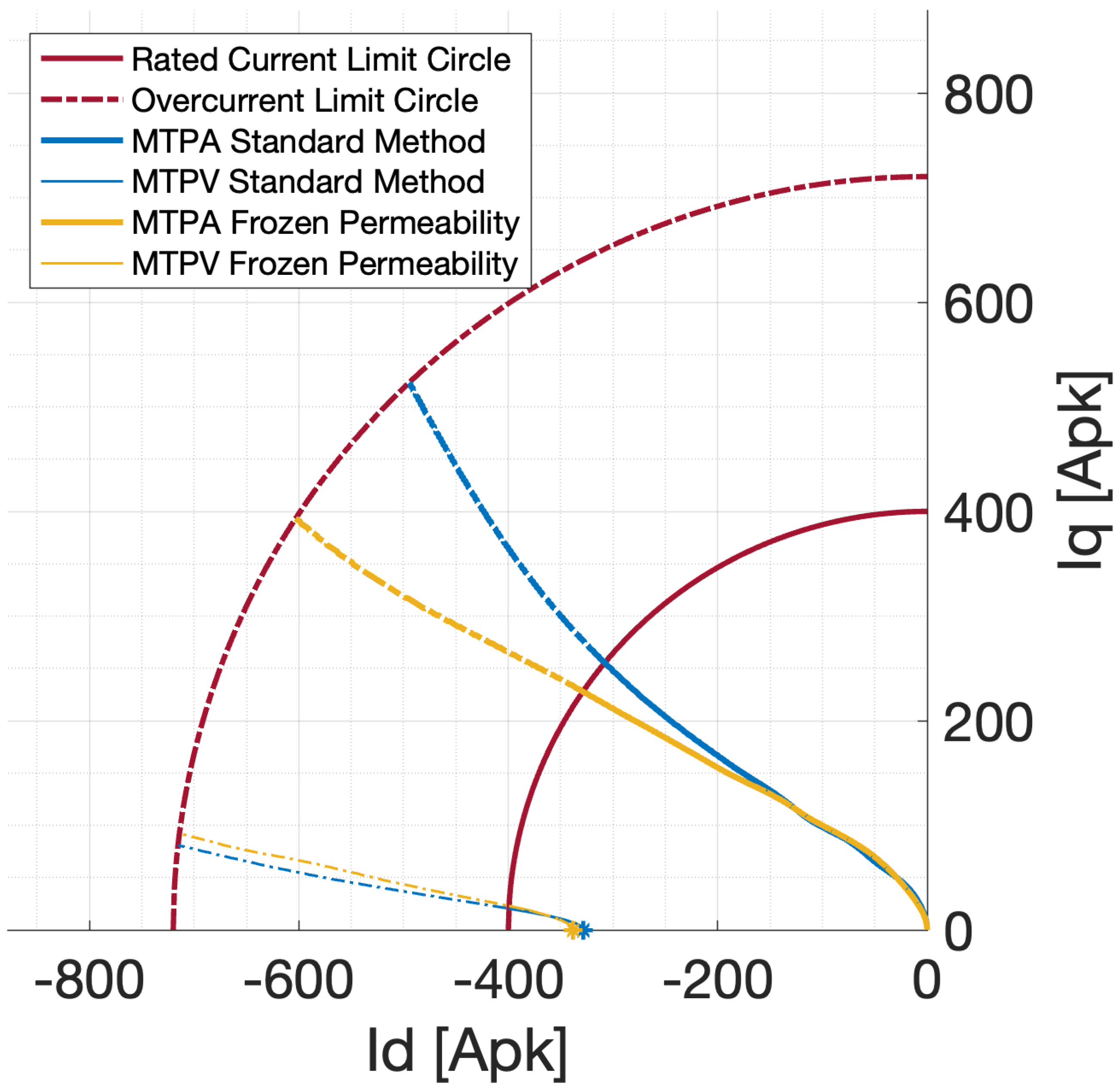
5.2. Comparison of the Two Different Nonlinear Methods

The comparison is further enhanced with a reference curve, based on trajectories computed with a 2-D FEA. Specifically, MTPA is computed by 2-D FEA FEMM with the following procedure:

• A range of current density $\left[J\right]$ is defined;
• A range of current phase angle $\left[\gamma \right]$ is defined;
• For each couple of $[J;\gamma ]$ matrix, five different rotor positions are defined (6 mechanical degrees apart one from the other in order to cover 360 electrical degrees);
• The solution of the magnetic model is found for all the different rotor positions and torque is evaluated by the Maxwell’s stress tensor;
• The mean value of the torque on all position is computed;

This process is repeated for each element $(J;\gamma )$. Then, MTPA trajectory is obtained computing the maximum torque value on all the values of $\gamma$.

Figure 14 shows a comparison between the MTPA curve obtained with: (i) the conventional linear model (green line); (ii) the nonlinear model based on standard magnetostatic simulations (blue line); (iii) the nonlinear model based on FP simulations (yellow line); (iv) the reference trajectory computed via 2-D FEA (purple line).

Results show that the MTPA trajectory is remarkably different for two nonlinear methods, especially at high currents (dashed lines). As shown, the reference 2-D FEA MTPA trajectory is much better matched with the MTPA obtained with FP method rather than with the one obtained with the Standard Method. The error for the linear model curve and for the Standard Method curve is significant especially outside the rated CLC, where the saturation effects are higher.

Regarding the output torque vs. speed characteristic, the comparison between linear model, standard nonlinear method and nonlinear FP is reported in Figure 15; in the constant torque region the three methods lead to a significant differences in the torque value, while in the constant power region the frozen permeability and the standard nonlinear methods lead to similar results. This is due to the effect of de-saturation linked with flux weakening.

In conclusion, FP method proves to be more accurate in the mapping and modeling of IPM synchronous machines.

6. Conclusions and Future Development

This paper presents a new algorithmic approach to compute the machine performance in MTPA, FW and MTPV for IPM synchronous machines. The proposed approach is applied to compute the current components in the $i_d-i_q$ reference frame for the MTPA, FW and MTPV, evaluating also the voltage limit ellipses, iso-torque curves, and torque vs. speed characteristic. Moreover, the proposed algorithms are efficient and suited to a real-time implementation, being still quite reliable in case of magnetic saturation

More traditional methods are based on a linear model, that does not account for $L_d$ and $L_q$ variations with the working point of the machine. Hence, traditional method fails at high speed, and/or with magnetic saturation, on the other hand a direct analytical solutions would require the computation of partial derivatives of $L_d(I,\gamma )$ and $L_q(I,\gamma )$ with respect to the current phase angle, leading to complex and unfeasible real-time implementations.

This paper proposes a method for MTPA, FW and MTPV that is efficient and suited to a real-time implementation, being still quite reliable in case of magnetic saturation.

The proposed method is based on the inductance maps of the machine obtained by 2-D Finite Element Analysis. Two different methods were adopted for the FEA simulations: a standard nonlinear magnetostatic method (Standard Method) and Frozen Permeability method (FP Method). The two solutions were assessed by a reference curve, obtained with a direct computation 2-D FEA via the Maxwell’s stress tensor. MTPA curve obtained with the conventional linear model differs significantly from the reference curve, especially for high currents values. On the other hand, the trajectory obtained with the proposed algorithmic approachis more similar to the reference. In addition to that, a comparison of the accuracy of the Frozen Permeability method with respect to the Standard Method was made.

Results prove the higher accuracy of the nonlinear model based on Frozen Permeability, especially in case of relevant currents and high saturation.

References

1. Yang, Z.; Shang, F.; Brown, I.P.; Krishnamurthy, M. Comparative Study of Interior Permanent Magnet, Induction, and Switched Reluctance Motor Drives for EV and HEV Applications. IEEE Trans. Transp. Electrif. 2015, 1, 245–254. [Google Scholar] [CrossRef]
2. Pellegrino, G.; Vagati, A.; Guglielmi, P.; Boazzo, B. Performance Comparison Between Surface-Mounted and Interior PM Motor Drives for Electric Vehicle Application. IEEE Trans. Ind. Electron. 2012, 59, 803–811. [Google Scholar] [CrossRef] [Green Version]
3. Grunditz, E.A.; Thiringer, T. Performance Analysis of Current BEVs Based on a Comprehensive Review of Specifications. IEEE Trans. Transp. Electrif. 2016, 2, 270–289. [Google Scholar] [CrossRef]
4. Bilgin, B.; Magne, P.; Malysz, P.; Yang, Y.; Pantelic, V.; Preindl, M.; Korobkine, A.; Jiang, W.; Lawford, M.; Emadi, A. Making the Case for Electrified Transportation. IEEE Trans. Transp. Electrif. 2015, 1, 4–17. [Google Scholar] [CrossRef]
5. Sarlioglu, B.; Morris, C.T. More Electric Aircraft: Review, Challenges, and Opportunities for Commercial Transport Aircraft. IEEE Trans. Transp. Electrif. 2015, 1, 54–64. [Google Scholar] [CrossRef]
6. Sulligoi, G.; Vicenzutti, A.; Menis, R. All-Electric Ship Design: From Electrical Propulsion to Integrated Electrical and Electronic Power Systems. IEEE Trans. Transp. Electrif. 2016, 2, 507–521. [Google Scholar] [CrossRef]
7. Jahns, T.M.; Kliman, G.B.; Neumann, T.W. Interior Permanent-Magnet Synchronous Motors for Adjustable-Speed Drives. IEEE Trans. Ind. Appl. 1986, IA-22, 738–747. [Google Scholar] [CrossRef]
8. Morimoto, S.; Takeda, Y.; Hirasa, T.; Taniguchi, K. Expansion of operating limits for permanent magnet motor by current vector control considering inverter capacity. IEEE Trans. Ind. Appl. 1990, 26, 866–871. [Google Scholar] [CrossRef]
9. Bianchi, N.; Jahns, T.M. Design, Analysis, and Control of Interior PM Synchronous Machines. In Proceedings of the IEEE Industry Applications Society, Seattle, WA, USA, 3–7 October 2004; Chapter 8. p. 1. [Google Scholar]
10. Bianchi, N. Electrical Machine Analysis Using Finite Elements, 1st ed.; CRC Press: Boca Raton, FL, USA, 2017. [Google Scholar] [CrossRef]
11. Stumberger, B.; Stumberger, G.; Dolinar, D.; Hamler, A.; Trlep, M. Evaluation of saturation and cross-magnetization effects in interior permanent-magnet synchronous motor. IEEE Trans. Ind. Appl. 2003, 39, 1264–1271. [Google Scholar] [CrossRef]
12. Guglielmi, P.; Pastorelli, M.; Vagati, A. Cross-Saturation Effects in IPM Motors and Related Impact on Sensorless Control. IEEE Trans. Ind. Appl. 2006, 42, 1516–1522. [Google Scholar] [CrossRef] [Green Version]
13. Miller, T.; Popescu, M.; Cossar, C.; McGilp, M. Performance estimation of interior permanent-magnet brushless motors using the voltage-driven flux-MMF diagram. IEEE Trans. Magn. 2006, 42, 1867–1872. [Google Scholar] [CrossRef] [Green Version]
14. Bojoi, R.; Cavagnino, A.; Cossale, M.; Vaschetto, S. Methodology for the IPM motor magnetic model computation based on finite element analysis. In Proceedings of the IECON 2014—40th Annual Conference of the IEEE Industrial Electronics Society, Dallas, TX, USA, 29 October–1 November 2014; pp. 722–728. [Google Scholar] [CrossRef]
15. Li, S.; Han, D.; Sarlioglu, B. Modeling of Interior Permanent Magnet Machine Considering Saturation, Cross Coupling, Spatial Harmonics, and Temperature Effects. IEEE Trans. Transp. Electrif. 2017, 3, 682–693. [Google Scholar] [CrossRef]
16. Chen, X.; Wang, J.; Griffo, A. A High-Fidelity and Computationally Efficient Electrothermally Coupled Model for Interior Permanent-Magnet Machines in Electric Vehicle Traction Applications. IEEE Trans. Transp. Electrif. 2015, 1, 336–347. [Google Scholar] [CrossRef]
17. Chen, X.; Wang, J.; Sen, B.; Lazari, P.; Sun, T. A High-Fidelity and Computationally Efficient Model for Interior Permanent-Magnet Machines Considering the Magnetic Saturation, Spatial Harmonics, and Iron Loss Effect. IEEE Trans. Ind. Electron. 2015, 62, 4044–4055. [Google Scholar] [CrossRef]
18. Li, Z.; Li, H. MTPA control of PMSM system considering saturation and cross-coupling. In Proceedings of the 2012 15th International Conference on Electrical Machines and Systems (ICEMS), Sapporo, Japan, 21–24 October 2012; pp. 1–5. [Google Scholar]
19. Li, S.; Sarlioglu, B.; Jurkovic, S.; Patel, N.; Savagian, P. Analysis of temperature effects on performance of interior permanent magnet machines. In Proceedings of the 2016 IEEE Energy Conversion Congress and Exposition (ECCE), Milwaukee, WI, USA, 18–22 September 2016; pp. 1–8. [Google Scholar] [CrossRef]
20. Consoli, A.; Scarcella, G.; Scelba, G.; Sindoni, S.; Testa, A. Steady-State and Transient Analysis of Maximum Torque per Ampere Control for IPMSMs. In Proceedings of the 2008 IEEE Industry Applications Society Annual Meeting, Edmonton, AB, Canada, 5–9 October 2008; pp. 1–8. [Google Scholar] [CrossRef]
21. Mademlis, C.; Agelidis, V. On considering magnetic saturation with maximum torque to current control in interior permanent magnet synchronous motor drives. In Proceedings of the 2002 IEEE Power Engineering Society Winter Meeting, Conference Proceedings (Cat. No.02CH37309). New York, NY, USA, 27–31 January 2002; Volume 2, p. 1234. [Google Scholar] [CrossRef]
22. Armando, E.; Guglielmi, P.; Pellegrino, G.; Pastorelli, M.; Vagati, A. Accurate Modeling and Performance Analysis of IPM-PMASR Motors. IEEE Trans. Ind. Appl. 2009, 45, 123–130. [Google Scholar] [CrossRef]
23. Hadžiselimović, M.; Štumberger, G.; Štumberger, B.; Zagradišnik, I. Magnetically nonlinear dynamic model of synchronous motor with permanent magnets. J. Magn. Magn. Mater. 2007, 316, e257–e260. [Google Scholar] [CrossRef]
24. Bianchi, N.; Bolognani, S. Magnetic models of saturated interior permanent magnet motors based on finite element analysis. In Proceedings of the Conference Record of 1998 IEEE Industry Applications Conference, Thirty-Third IAS Annual Meeting (Cat. No.98CH36242). St. Louis, MO, USA, 12–15 October 1998; Volume 1, pp. 27–34. [Google Scholar] [CrossRef]
25. Lopez-Torres, C.; Bacco, G.; Bianchi, N.; Espinosa, A.G.; Romeral, L. A Parallel Analytical Computation of Synchronous Reluctance Machine. In Proceedings of the 2018 XIII International Conference on Electrical Machines (ICEM), Alexandroupoli, Greece, 3–6 September 2018; pp. 25–31. [Google Scholar] [CrossRef]
26. Hoang, K.D.; Aorith, H.K.A. Online Control of IPMSM Drives for Traction Applications Considering Machine Parameter and Inverter Nonlinearities. IEEE Trans. Transp. Electrif. 2015, 1, 312–325. [Google Scholar] [CrossRef] [Green Version]
27. Yan, Y.; Zhu, J.; Lu, H.; Guo, Y.; Wang, S. Study of A PMSM Model Incorporating Structural and Saturation Saliencies. In Proceedings of the 2005 International Conference on Power Electronics and Drives Systems, Kuala Lumpur, Malaysia, 28 November–1 December 2005; Volume 1, pp. 575–580. [Google Scholar] [CrossRef]
28. Yan, Y.; Zhu, J.; Guo, Y.; Lu, H. Modeling and Simulation of Direct Torque Controlled PMSM Drive System Incorporating Structural and Saturation Saliencies. In Proceedings of the Conference Record of the 2006 IEEE Industry Applications Conference Forty-First IAS Annual Meeting, Tampa, FL, USA, 8–12 October 2006; Volume 1, pp. 76–83. [Google Scholar] [CrossRef] [Green Version]
29. Liu, Z.; Feng, G.; Han, Y. Extended-Kalman-Filter-Based Magnet Flux Linkage and Inductance Estimation for PMSM Considering Magnetic Saturation. In Proceedings of the 2021 36th Youth Academic Annual Conference of Chinese Association of Automation (YAC), Nanchang, China, 28–30 May 2021; pp. 430–435. [Google Scholar] [CrossRef]
30. Park, G.; Kim, G.; Gu, B.G. Sensorless PMSM Drive Inductance Estimation Based on a Data-Driven Approach. Electronics 2021, 10, 791. [Google Scholar] [CrossRef]
31. Wu, H.; Zhao, W.; Zhu, G.; Li, M. Optimal Design and Control of a Spoke-Type IPM Motor with Asymmetric Flux Barriers to Improve Torque Density. Symmetry 2022, 14, 1788. [Google Scholar] [CrossRef]
32. Dorrell, D.G. On the Use of the Frozen Permeability Method for Torque Separation in Synchronous Machines Invited Oral Poster. In Proceedings of the 2016 International Conference of Asian Union of Magnetics Societies (ICAUMS), Tainan, Taiwan, 1–5 August 2016; pp. 1–4. [Google Scholar] [CrossRef]
33. Chen, J.; Li, J.; Qu, R.; Ge, M. Magnet-Frozen-Permeability FEA and DC-Biased Measurement for Machine Inductance: Application on a Variable-Flux PM Machine. IEEE Trans. Ind. Electron. 2018, 65, 4599–4607. [Google Scholar] [CrossRef]
34. Neumann, J.; Hénaux, C.; Fadel, M.; Prieto, D.; Fournier, E.; Yamdeu, M.T. Improved dq model and analytical parameters determination of a Permanent Magnet Assisted Synchronous Reluctance Motor (PMa-SynRM) under saturation using Frozen Permeability Method. In Proceedings of the 2020 International Conference on Electrical Machines (ICEM), Gothenburg, Sweden, 23–26 August 2020; Volume 1, pp. 481–487. [Google Scholar] [CrossRef]
35. Shuto, D.; Takahashi, Y.; Fujiwara, K. Frozen Permeability Method for Magnetic Field Analysis of Permanent Magnet Motors Considering Hysteretic Property. IEEE Trans. Magn. 2019, 55, 1–4. [Google Scholar] [CrossRef]
36. Meeker, D. Finite Element Method Magnetic. User’s Manual. 2018. Available online: https://www.femm.info/wiki/HomePage (accessed on 16 May 2020).
Figure 1. MTPA, FW and MTPV trajectories on d-q reference frame.
Machines 11 00077 g001
Figure 2. Geometry of the reference IPM synchronous machine.
Machines 11 00077 g002
Figure 3. Inductance map of d-axis ( L d ) obtained with the Standard Method.
Machines 11 00077 g003
Figure 4. Inductance map of q-axis ( L q ) obtained with the Standard Method.
Machines 11 00077 g004
Figure 5. Inductance map of d-axis ( L d ) obtained with the Frozen Permeability method.
Machines 11 00077 g005
Figure 6. Inductance map of q-axis ( L q ) obtained with the Frozen Permeability method.
Machines 11 00077 g006
Figure 7. Procedure of the FW algorithm on the d-q reference plane.
Machines 11 00077 g007
Figure 8. Procedure of MTPV algorithm on the new D-Q reference plane.
Machines 11 00077 g008
Figure 9. Control trajectories on the d-q plane computed with a Standard Method.
Machines 11 00077 g009
Figure 10. Control trajectories on the d-q plane computed with FP.
Machines 11 00077 g010
Figure 11. Control trajectories on the d-q plane computed with the conventional linear model.
Machines 11 00077 g011
Figure 12. Comparison of MTPA and MTPV curves, obtained with Standard Method (blue) and FP (yellow).
Machines 11 00077 g012
Figure 13. Comparison of Voltage Limit Ellipse (at base speed) and Constant Torque Hyperbola (at rated torque), obtained with Standard Method (blue) and FP (yellow).
Machines 11 00077 g013
Figure 14. Comparison of MTPA curve obtained by the conventional linear model, nonlinear model based on Standard Method, nonlinear model based on FP and direct computation via 2D FEA.
Machines 11 00077 g014
Figure 15. Comparison of torque–speed curves obtained by the conventional linear model, nonlinear model based on Standard Method and nonlinear model based on FP.
Machines 11 00077 g015