Article

Stress and Corrosion Defect Identification in Weak Magnetic Leakage Signals Using Multi-Graph Splitting and Fusion Graph Convolution Networks

College of Information Science and Engineering, Northeastern University, Shenyang 110819, China
*
Author to whom correspondence should be addressed.
Machines 2023, 11(1), 70; https://doi.org/10.3390/machines11010070
Submission received: 21 November 2022 / Revised: 29 December 2022 / Accepted: 3 January 2023 / Published: 6 January 2023
(This article belongs to the Section Machines Testing and Maintenance)

Abstract

:
Weak magnetic flux leak detection is one of the most important non-destructive testing and measurement methods for pipelines. Since different defects cause different damage, it is necessary to classify the different types of defects. Traditional machine learning methods of defect type identification mainly use feature analysis methods and rely on expert a priori knowledge and the ability of designers. These methods have the following weaknesses: a priori knowledge needs to be designed iteratively, and a priori knowledge design relies on expert experience. In recent years, the rapid development of deep learning methods in the field of machine vision has led to the development of defect analysis in the industry. However, most deep learning methods lack the ability to analyze both detailed information and the overall structure. In this paper, we propose graph convolution networks for splitting and fusing multiple graphs of detail graphs and a root graph. Detail information (detail graphs) provides detailed information for the detection of WMFLs. The structure information (root graph) provides structural information for the detection of WMFLs. This paper uses simulation data and experimental data to verify that the proposed method can identify stress defects and corrosion defects well. The paper explains the experimental results in detail to demonstrate the superiority of the method in industrial methods.

1. Introduction

The weak magnetic flux leakages (WMFLs) detection [1] method is a novel pipelines non-destructive detection method. Pipeline corrosion (corrosion defects) [2] can lead to pipeline ruptures and oil and gas leaks [3,4]. Pipeline stress imbalances (stress defects) [5] can lead to ruptures, excessive deformation and pipeline buckling [6,7]. The magnetic distribution of stress defects and corrosion defects is recorded as the internal detector passes through the pipelines being inspected [8]. Different types of defects require different defect assessment methods and different engineering maintenance methods. Therefore, it is necessary to identify different defects in engineering and treat each separately. Misidentification of the WMFLs signals caused by stress defects and corrosion defects may lead to serious engineering consequences.
The identification of stress and corrosion defects is an important process. If a stress defect is incorrectly identified as a corrosion defect, the pipelines may deform excessively and rupture. Conversely, if the corrosion lack of corrosion is identified as stress defects, the worst case may result in pipelines destroyed because of corrosion. Identification problems can be divided into two categories, including the use of detailed information and the use of structural information.
Figure 1 shows an example of real WMFLs signals. Figure 1a shows a chemically corroded corrosion defect and its corresponding WMFLs. The length and width of the defect are 10 mm and 20 mm, respectively, and the depth is about 50% of the wall of the pipeline. Figure 1b shows a production environment with stress defects and its corresponding WMFLs. It can be seen that the WMFL signals of stress defects and WMFL signals of corrosion defects are very similar.
In order to identify defect types from complex WMFL detection signals, many identification methods based on detailed information have been developed, such as statistical analysis [9], convolutional neural networks [10], and wavelet transforms [11]. Detail information is a different feature extracted multiple times from one WMFL detection signal. For example, the convolutional kernel of a convolutional neural network [12] can extract different detail information at different locations of the WMFL detection signals. Identification methods that use structural information are identified by analyzing non-repetitive features in the same WMFL detection signals, such as the results of physical models or features extracted based on expert experience [13]. It can be a physical model or feature-based machine learning methods [14].
Detail information includes the effect of details caused by the magnetic flux leakage mechanism and the effect of useless details caused by noise. The structure information is the profile information of WMFL signals, which can reflect the underlying structure of the magnetic leakage detection information. If only detail information is used to identify corrosion defects and stress defects, noise may affect identification. If only structural information is used to identify corrosion defects and stress defects, the difference in structural information may not be sufficient to complete the identification. Neither detail information nor structural information is sufficient to analyze defect types alone.
In this paper, our goal is to develop a method for the identification of stress defects and corrosion defects using detail information and structural information. The main difference between WMFL signals of stress defects [15] and WMFL signals of corrosion defects [16] is the difference in the weak magnetic flux leakage mechanism. The most critical differences between WMFLs signals of stress defects and WMFLs signals of corrosion defects include detail differences and structural differences. In this paper, a new detail-based and structure-based graph method is proposed, which improves the feature-based information identification. Graph convolutional networks (GCNs) are used for the analysis and identification of relational information. The method proposed in this paper can use both detail information and structure information as input.
The main contributions are summarized as follows:
  • A multi-graph splitting and fusion of detail graphs and the root graph are proposed to change the deficiency that graph convolutional networks cannot cope with both detail and structure information. The root graph can capture the structure relationship of the WMFLs detection information. The detail graphs can capture the detailed features of the WMFLs detection information. By using the fusion of multiple root graph and detail graphs, the method proposed in this paper can analyze both the structure and detailed features of the detection information.
  • Compared with the typical GCNs method, the multi-graph splitting and fusion GCNs method can transform more detection details by splitting and more overall information by fusion. Although multi-graph splitting and fusion GCNs have the limitation of increasing training costs, the method uses larger-scale spatial information for analysis and to some extent extracts information from smaller-scale information re-fusion methods.
  • We used two experiments to verify the effectiveness of our proposed method. First, this paper compares the detection results of multi-graph splitting and fusion GCNs and typical GCNs. Secondly, this paper compares traditional machine learning methods based on expert experience and feature engineering with our proposed method. The results show that the multi-graph splitting and fusion graph GCNs method is better than the typical GCNs method. Meanwhile, compared with traditional machine learning methods, multi-graph splitting and fusion GCNs can identify defects better.
The rest of this paper is organized as follows. In Section 2, the basic mechanism and structure of weak flux leakage detection are presented. In Section 3, we describe the proposed multi-graph splitting and fusion graph method for identifying stress defects and corrosion defects. In Section 4, the validation dataset including simulation data and experimental data is described. In Section 5, we validate the superiority and practicality of the multi-graph splitting and fusion graph method proposed in this paper. Finally, conclusions are given in Section 6.

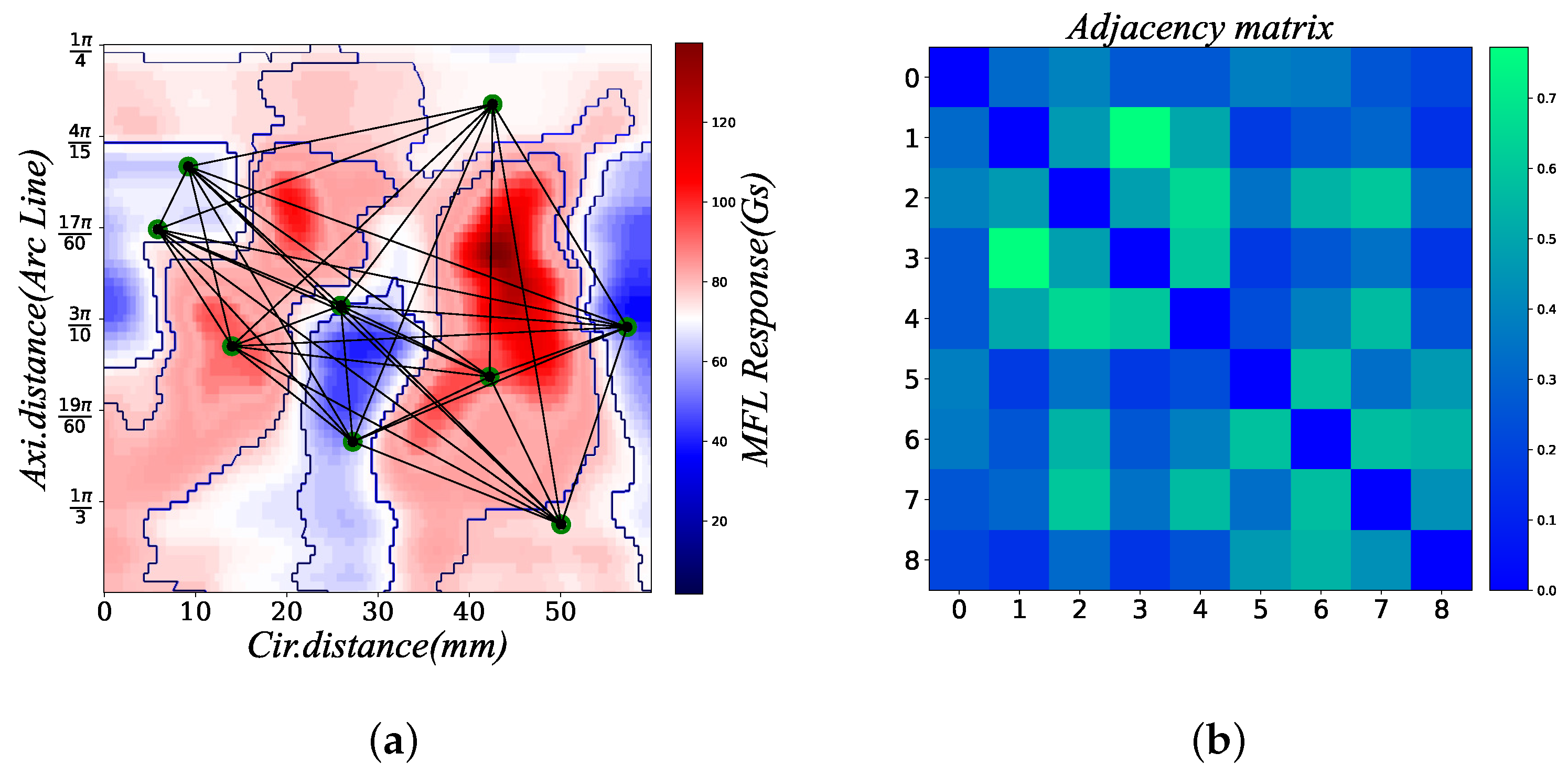
2. Principle of WMFLs Testing

As shown in Figure 2, the mechanical structure of the WMFLs detector is a plurality of individual cylinders connected to each other. The whole WMFLs detector is divided into three parts: the battery part, detection part and recording part [4,17]. In contrast to saturated excitation [18] of the internal WMFLs detectors, the weak excitation method requires the use of weak excitation [19] or geomagnetic excitation [8] to excite the WMFLs signals. Weak permanent [20] magnets magnetize the corrosion defects and stress defects in the pipeline’s wall. The magnetic field at the defect location is leaked. Hall sensors detect the magnetic field and then record the part to save the magnetic field and the corresponding location. WMFLs internal detectors detect the pipelines while being pushed by pressure inside the pipelines. After the inspection at the end of the pipelines is completed, it is removed from the end of the pipelines and taken back to the laboratory. After filtering and pre-processing, WMFLs data are obtained.
Many factors such as excitation [21], magnetic circuit [22], detection method [8,23], material characteristics [24], etc. directly affect the WMFLs signals. In actual industrial inspection, various uncontrollable field conditions (e.g., internal detector lift-off values [25] in the pipelines, excitation, magnetic circuit, material properties) affect the WMFLs signals. In detection pipelines where WMFLs detectors are pushed, small vibrational displacements can cause lift-off value variation problems at the sensor level. A discrete sampling of continuous WMFLs signals can change the representation of WMFLs information. Therefore, WMFLs signals of stress defects and WMFLs signals of corrosion defects require spatially-based analysis methods.
Traditional feature extraction methods lack intelligent methods based on data identification. The use of deep learning as a basic method cannot handle spatial information. From the above analysis, it can be seen that the existing methods cannot solve the problem of classifying WMFLs signals of stress defects and corrosion defects. A new distance-based method should be found to solve the problem and improve the accuracy of estimation.

3. Architecture of the Proposed Model

Information in the real world is mainly unstructured information, and graphs are the most intuitive way to express it. Compared to Euclidean structured data (image), graphs can provide more information [26]. Graph convolutional networks were first proposed by the literature [27]. Typical GCNs can analyze more non-neighborhood information than convolutional methods that use only convolutional kernels. This method is probably one of the most effective methods for analyzing WMFLs signals caused by stress imbalance changes and corrosion-induced WMFLs signals.
The organization of WMFLs data as structured data and not unstructured data is the reason why typical GCNs cannot be directly used for identification. In pipeline WMFLs detection, a sensor mounted on an internal detector passes through the area where the WMFLs signals change. These signals are recorded in the computer memory as structural data based on the distance traveled and the pipeline angle. Some studies directly apply deep learning methods by converting WMFLs data into gray or pseudo-color images, but such images are still structural data [3,4]. These methods also cause a loss of spatial information of the signals. For example, the trend of small amplitude variation of WMFLs signals for stress defects and corrosion defects is directly related to the spatial distance. Deep learning methods that convert WFLs signals to grayscale and pseudo-color images typically ignore these details.
To solve the above problem, a new method is proposed in this paper. We use superpixel-like information fusion to convert structured WMFLs signals into unstructured graphs. A multi-level graph convolutional network is proposed based on splitting and fused graph convolution. The structure of the new method includes splitting and multilevel graph convolution, and the overall result is shown in Figure 3.

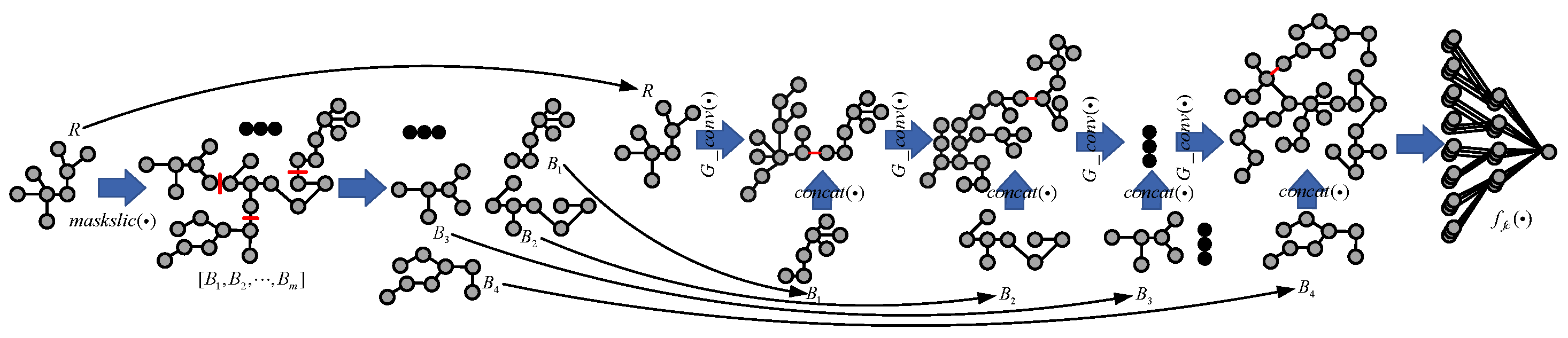
3.1. First Split, Re-Split and Graph Fusion Convolution
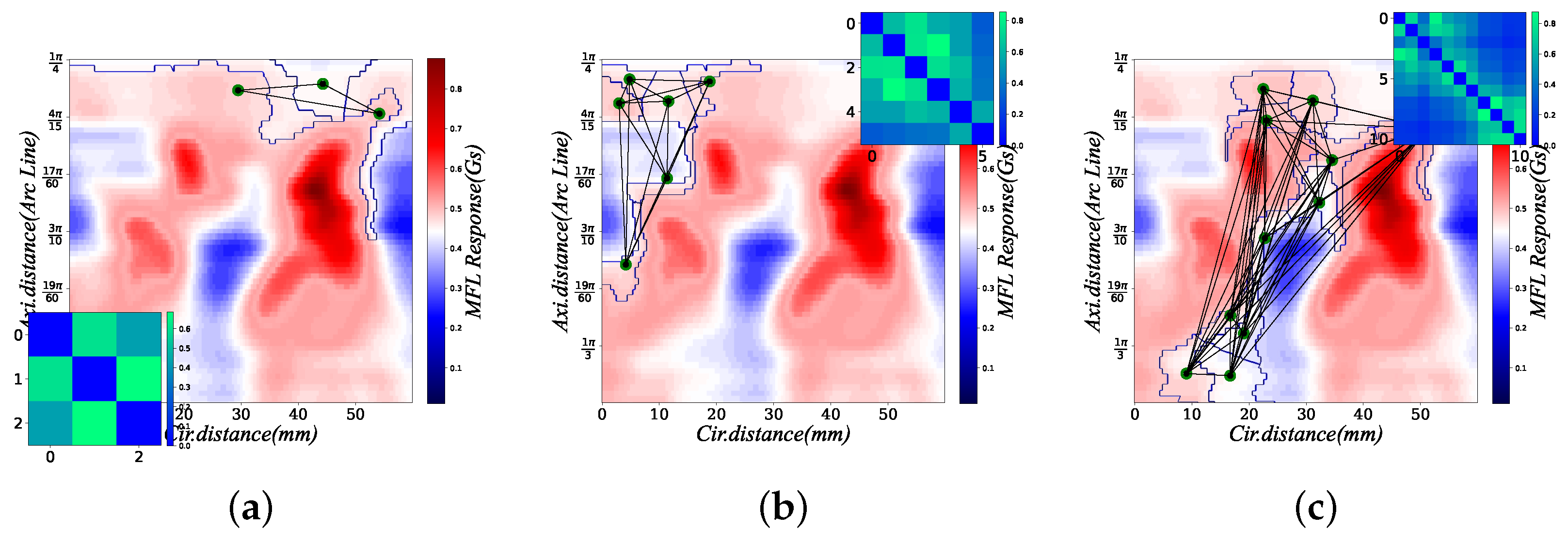
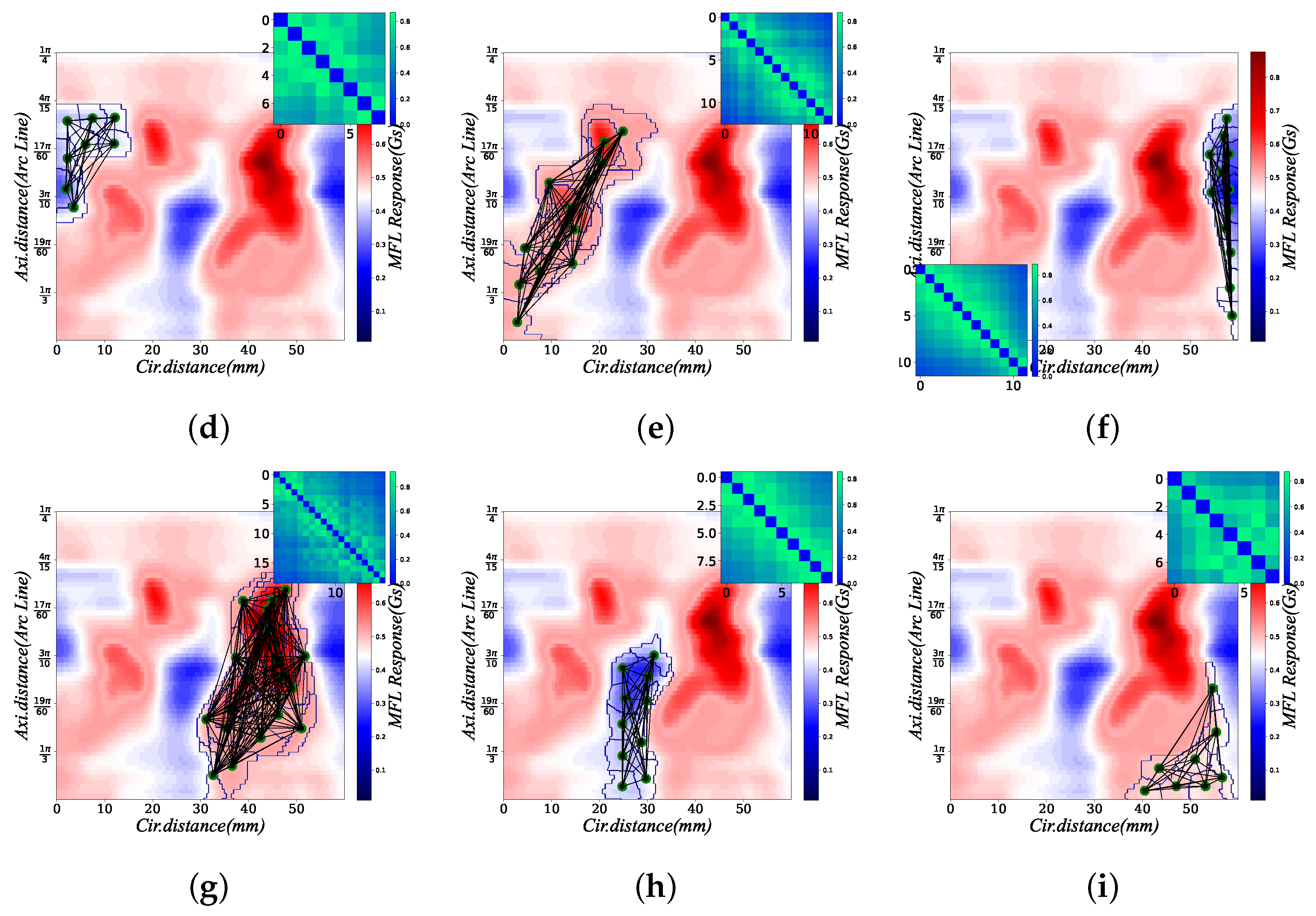
3.1.1. Twice-Split

The graph multi-graph splitting and fusion is a novel graph convolution networks structure. This method changes the scale characteristics of the information fusion graph convolution. As shown in Figure 4, the first-split is the step of abstraction of structured data into an unstructured root graph. Re-split is the step of transforming the unstructured root graph into unstructured detail graphs. It can maintain a similar number of parameters and computational cost as high-level information fusion. The graph twice-split consists of two parts, the first-split and the re-split. The result of the multi-graph splitting and fusion unstructured detail graphs is a sub-part of the unstructured root graph.
The first-split is the conversion of the WMFLs signals’ structured data into the root graph using the superpixel method [28]. Then, the sub-nodes of the root graph are converted to unstructured detail graphs by the maskSLIC method [29]. The first-split and re-split method changes the scale characteristics of the graph convolution. It allows the unstructured detail graphs to maintain a similar number of parameters and computational cost as the unstructured root graph. The first-split and re-split are very flexible and scalable. As show in Figure 5, each detail graph is a sub-node of the graph node in Figure 4. Unstructured detail graphs can better describe the detection details, and the root graph can better describe the overall detection.

3.1.2. Graph Fusion Convolution

The input of the graph fusion is divided into two parts. The first part is the analysis result of the last graph convolution operation. The second part of the graph fusion is unstructured detail graphs. The result of the graph fusion is the fusion of the two parts of information. The first part of the graph fusion graph convolution result can be seen as a valid but complex information derivation.
c o n c a t ( ) is the method of joining two graphs:
X ¯ = c o n c a t ( X , B )
where X ¯ is the root graph and input of the graph convolutional first layer of multi-graph splitting and fusion GCNs, and X is the output of the graph convolution, where B is the unstructured detail graphs.
As shown in Figure 3, these results can be considered as a new graph. c o n c a t ( ) is a simple method, but this method changes the overall structure of the multi-graph splitting and fusion GCNs networks. Both the adjacency matrix A and the degree matrix D are simultaneously inflated with c o n c a t ( ) , which is equivalent to the expansion of the graph structure.
X 0 = R X ¯ k 1 = c o n c a t ( X k 1 , B k 1 ) , i [ 1 , M ] X k = σ k 1 D 1 2 A D 1 2 X ¯ k 1 W k Y = f f c ( X m )
where R is the root graph and input of the graph convolutional first layer of multi-graph splitting and fusion GCNs, W k represents the weights that can be trained in the k t h layer, and σ k and f f c are the activation functions and fully connected layer. The method used by σ k in this paper is R E L U ( ) function, where D is the degree matrix, and A is the adjacent matrix.
It should be noted that this paper still uses the results of the transformation of two fully connected layers, which can be considered as concatenation and projection [30]. The previous assumption was that each graph corresponds to an adjacency matrix. The correspondence between this graph and the adjacency matrix is implicit in the preconditioner. It is important to know that the assumption is based on the premise that the space corresponding to the features is constant.
Each graph convolution is followed by an insertion graph fusion structure. The graph convolution after each inserted detail graph transforms the inserted detail graphs and the original graph into a new graph. These information fusion results are analyzed by graph convolution for the types of defects. In the whole structure, this paper uses nine convolutions and nine fusions. The input of the first nine convolutions and interpolations is unstructured detail graphs. At the end of the networks, this paper uses a fully connected layer to transform elements and results.

3.2. Graph Convolution

Although the deep learning method ignores the location relationship of actual spatial information, the biggest advantage of multi-graph splitting and fusion GCNs is that it can extract non-expert and non-visual experience features by convolutional operations. In graph convolution theory, the graph convolution method can extract and analyze the relationship between unstructured data. The graph convolution method is also an essential and important step. The fundamental purpose of multi-graph splitting and fusion GCNs is to extract the features of unstructured data. Another advantage of multi-graph splitting and fusion GCNs is the naturalness of relationships in modeling. Each node in the graph changes the convolution kernel by the relationship between neighbor nodes and non-neighbor nodes during the training process. The measurement of this relationship is completed by the convolution kernel.

3.3. Global Pooling and Fully Connected Layer

The large number of parameters of deep learning methods leads to computational difficulties and memory explosions. This problem is alleviated by graph pooling methods, which are an integral part of the graph convolution networks method. In image data, the pooling method is very attractive. The biggest feature of the pooling method is a large number of parameter inputs and parameter downsampling. Generally, the pooling method of graph convolutional networks is mainly through clustering methods, which are very computationally intensive. Second, the information fusion method of the root and detail graphs split method proposed in this paper completes partial information downsampling. At the same time, the existing research lacks the analysis of clustering advantages. We use a gPool method [31] at the last layer to pool the information.
The last pooling layer is mainly completed by the graph pooling operator of the graph Fourier transform. The advantages and disadvantages of the method in the algorithm are also obvious. The main method and rule structure for clustering pooling is to run the clustering algorithm on each graph individually. This approach narrows the field of acceptance and extracts more accurate information.
y i = x i p / p
After completing the convolution of the child graph, we directly connect the fully connected networks and the R E L U ( ) activation function to convert the convolution result.
Z = f f c ( y i )
The structural framework of the networks is shown in the Figure 3. Multi-graph splitting and fusion GCNs creates a multi-graph convolution and fusion structure. The overall structure can also be considered as a multi-graph convolution with continuous fusion. The input of multi-graph splitting and fusion GCNs is the root graph, and the graph fused with the graph convolution result is the detail graphs. Each graph convolution is followed by an expansion structure, and the result of graph convolution is merged by expansion and new graph convolution. After each expanded structure, a new graph will be obtained, and we will set the expansion result as the expansion of the number of nodes in the graph. The result of multiple expansions is to complete all the transformed non-structural information that expresses the transformation of all structural information through the networks. In the whole structure, we used nine times of convolution and nine times of dilation. At the end of the networks, we use a fully connected layer to transform features and results.

4. Dataset Details

4.1. Simulation Dataset

The dataset is necessary to analyze the model. The simulation dataset includes the WMFLs dataset of stress defects and WMFLs dataset of corrosion defects. The WMFLs dataset of stress defects is composed of 15,000 simulated WMFLs signals; the WMFLs dataset of corrosion defects is composed of 15,000 simulated WMFLs signals.

4.1.1. Stress Defect

The phenomenon of mechanical degradation of non-linear magnetic detection ferromagnetic elements conforms to the villari effect [32]:
H e f f = H + 3 λ s μ 0 M s 2 S e d M , S e d = dev c H : ϵ e l
where the hysteresis magnetization strength M a n is
M a n ( H , σ ) = M s coth H e f f a a H e f f
where M s is the saturation magnetization strength, H is the external magnetic field, M is the magnetization strength, c H is the stiffness matrix measured under a constant magnetic field, λ s is the saturation magnetostriction, and ϵ e l is the material strain.
As shown in Figure 6, the types of stress defects include the simulation of eight contact situations between objects and pipelines. These contact conditions include: the mutual extrusion of the pipeline and spheres, the mutual extrusion of the pipeline and the cone, the mutual extrusion of the pipeline and cubes, the mutual extrusion between the pipeline and a coarse cylinder, and the mutual extrusion between a pipe and a fine cylinder. The displacement direction is the direction perpendicular to the surface of the pipeline’s wall that the object touches. It is possible to simulate the extrusion of the contact object on the wall of the pipelines. The randomly emulated squeeze is randomly generated for less than 1 cm.

4.1.2. Corrosion Defect

The WMFLs signals of corrosion defects is usually calculated mathematically using a magnetic dipole. Feng [4] proposed a method to simulate corrosion defects at arbitrarily different depths. The magnetic field d H generated at distance r by each element of charge d p = σ d y d z is given in:
d H ( x , y , z ) = d p 4 π r 3 r
As shown in Figure 7, corrosion defects are classified as rectangular defects and elliptical defects. The first part of the simulated dataset is regular rectangular corrosion. The length and width of the defect are randomly selected between 1 and 10 cm. The depth of the defect is also randomly selected between 0.1 mm and 0.9 cm. The second part is irregular defects. Irregular defects can be divided into multiple independent defects of different depths. The sum of the magnetic response H at each different depth is calculated cumulatively at each given point H i n d .
H = i j H i n d
where n and m represent the size of the mesh. The length and width of the defect are randomly selected between 1 and 10 cm. The deepest depth of the irregular defect is chosen randomly between 0.1 and 1 cm.

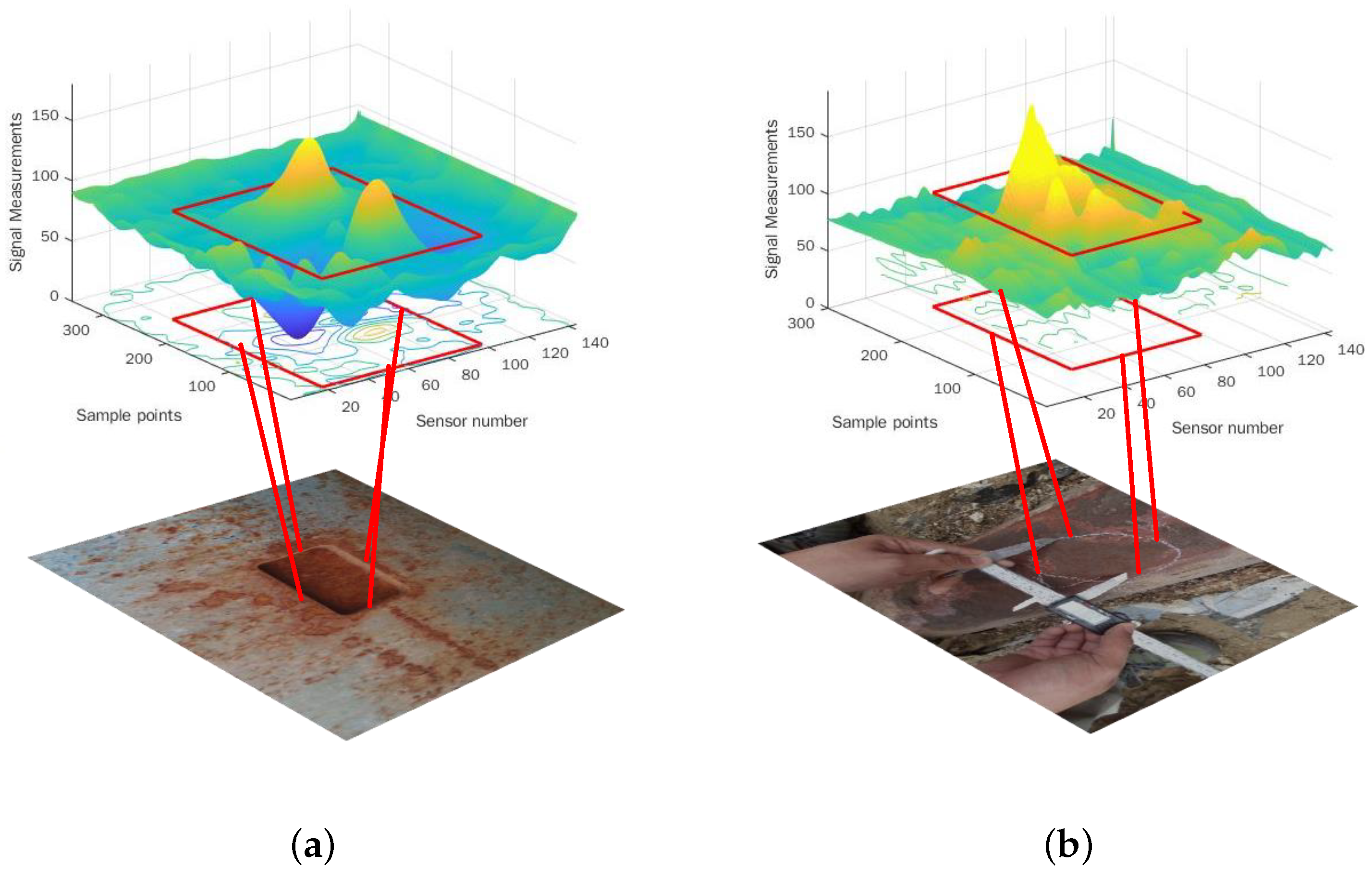
4.2. Experimental Dataset

In order to obtain the experimental dataset, the pipeline experiment platform and the production environment are used to obtain the data. The pipeline experiment platform is shown in Figure 8a. It has 67 pipelines of X65 steel with a diameter of 8 inches. There are a total of 150 stress defects in the pipeline. The experimental dataset has 300 WMFLs signals of stress defects and 700 WMFLs signals of corrosion defects. As shown in Figure 8b–d, there are a total of 300 stress defects, 30 of which come from the pipeline experiment platform and the rest come from the production environment. The stress defects generated in the production environment are mainly caused by geological movements [33]. It includes changes in the stress state of pipelines caused by earthquakes [33], landslides [34], loess collapse [35], thawing and settling of permafrost [36]. Half of the corrosion defects WMFLs signals came from the production environment (350), and the other half came from the experimental platform (350). As shown in Figure 8e, part of the signals caused by corrosion was obtained by chemical etching at the experimental platform, and its length and width ranged from 10 to 60 mm. The depth varies between 0.1 and 0.9 cm. As shown in Figure 8d, the corrosion is uniformly distributed, but in reality, it is randomly distributed. We also selected some of the corrosion signals collected during the actual inspection.

5. Experiment

We designed some comparative experiments to verify the ability of the proposed method in this paper to identify WMFLs signals of stress defects and WMFLs signals of corrosion defects. First, we analyzed the defect identification ability of multi-graph splitting and fusion GCNs and typical GCNs. Then, traditional machine learning methods based on expert experience and feature engineering are compared with our proposed approach. These experiments demonstrate the advanced performance of our proposed method.

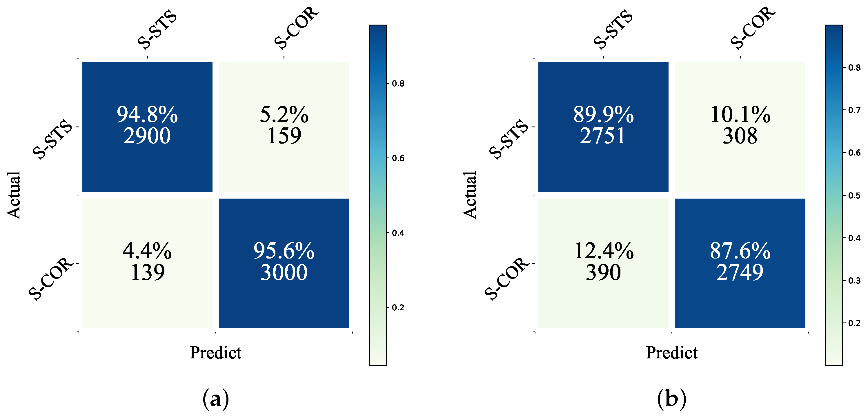
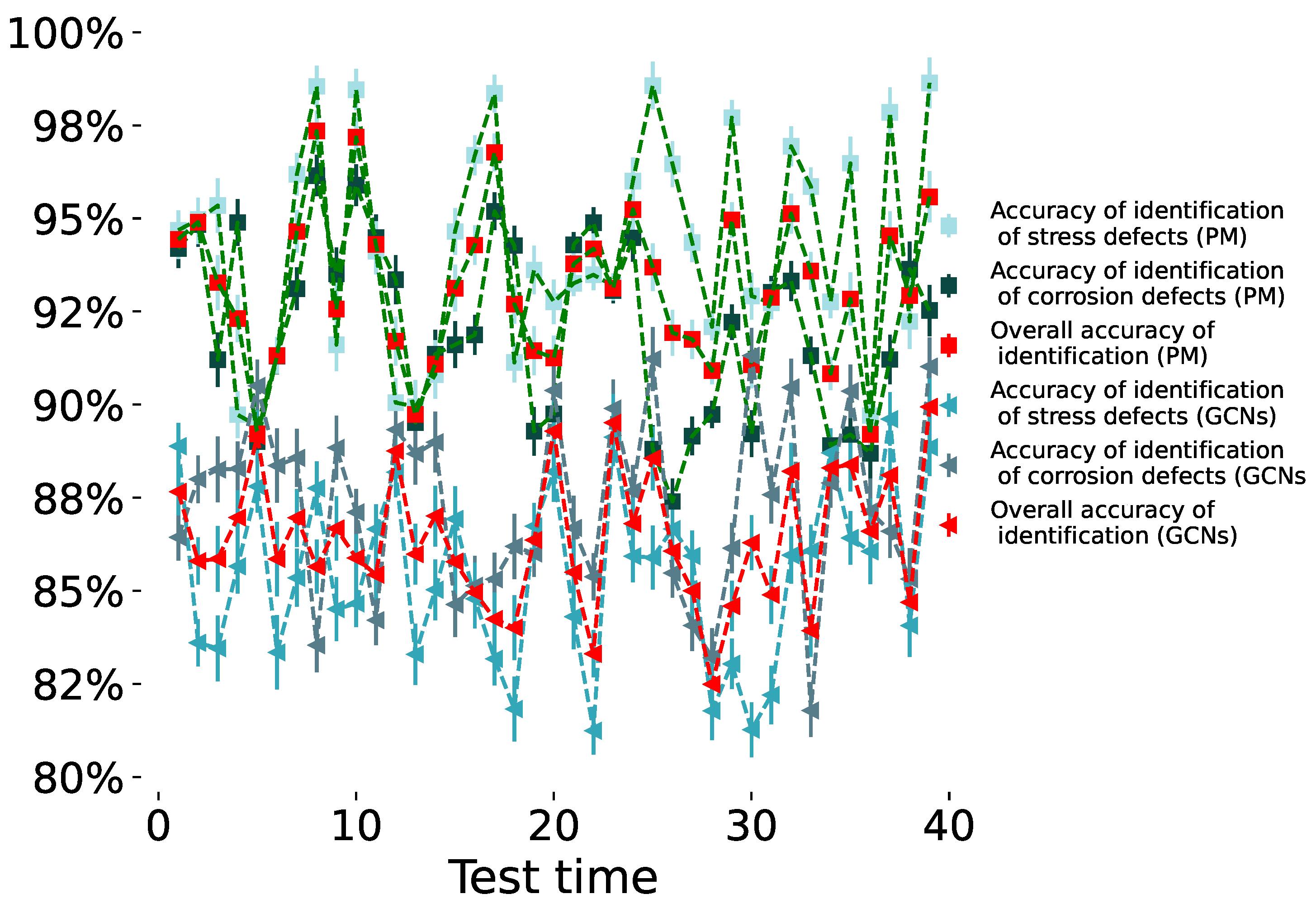
5.1. Analysis of the Validity of Our Proposed Method

In Section 3.1, this paper introduces a graph fusion convolution algorithm based on two splits. In order to illustrate the advantages of our proposed multi-graph splitting and fusion GCNs, the proposed algorithm in this paper is compared with typical GCNs for experiments. Since the detection results of WMFLs signals are structured data, the detection data are converted to unstructured data by a super-pixel method, and the defect type is used as the output. The data used for training and testing are the simulation datasets suggested in Section 4.1. We randomly allocate 80% of the dataset to training and randomly assign 20% of the dataset to testing. The average result of all five experiments is shown in Figure 9.
In order to verify that our proposed method can be better applied in a practical detection environment, the experimental data in Section 4.2 and the simulation data in Section 4.1 are used for the comparison experiments. The training dataset consists of the simulation data and the experimental data, and the test dataset consists of the experimental dataset. The specific training datasets and test datasets are described by Table 1.
In Figure 9a,b, the identification accuracy of our proposed method is better than the accuracy of typical GCNs. In industrial applications, the identification accuracy is the most important aspect. It can be seen that the identification accuracy of the proposed method in this paper is 95.12% on average in real industrial applications. Compared with the identification accuracy of the proposed method in the simulation data, the identification accuracy in the actual industrial application is only reduced by 1%. Therefore, the method proposed in this paper can solve real industrial problems.
In Section 3, multi-graph splitting and fusion GCNs are proposed. Information splitting and information multiple fusion are used to illustrate the advantages of the structure of our proposed networks. We compare our proposed method with a typical GCNs method. For typical GCNs, the structural magnetic flux leakage signals are converted to unstructured data by an information fusion method with the defect type as the output. The dataset used for training and testing is the simulated dataset described by Section 5. Five five-fold crossover experiments have been completed. The average accuracy of each test is shown in Figure 10.

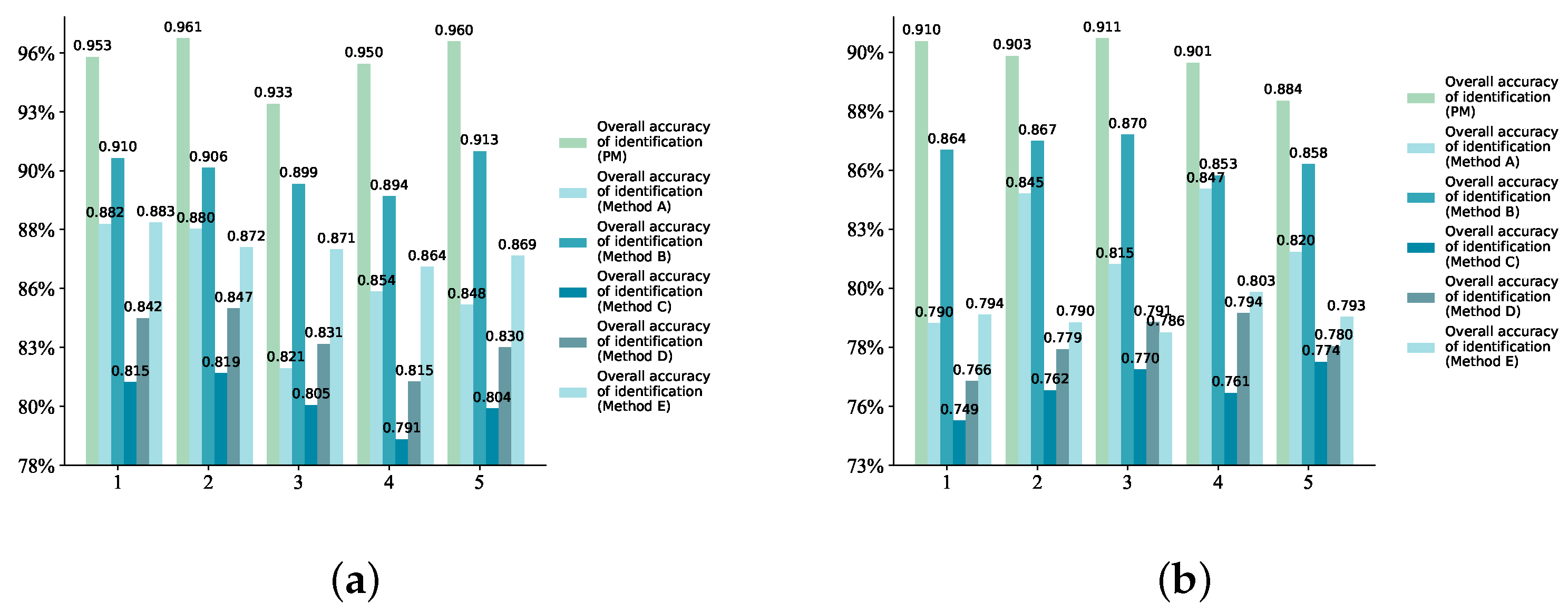
5.2. Comparison of Different Method

In order to prove that our proposed method is more effective than the traditional machine learning method, some experiments on different methods are conducted in this paper. A CNN method [3] is used for identifying injurious and non-injurious defects, which can be used to identify stress defects and corrosion defects. Method A is the original CNNs method [3]. The proposed method in this paper is mismatched compared to CNNs of this scale. Method B is an extension of the networks proposed [3]. The structure of two-layer CNNs was changed to five-layer CNNs. In order to demonstrate the superiority of the method, a comparison between the method and the traditional method is completed in this paper. Conventional methods are usually based on the feature [14,37] of the measured WMFLs signals to identify stress defects and corrosion defects. These conventional methods usually require expert experience to determine the selection of features and calculate hyperparameters. The proposed method in this paper has been compared with method C (support vector machine) [38], method D (back-propagation neural networks) [39], and method E (randomized decision trees) [40]. Method C is a support vector machine method that uses radial basis functions as kernel functions. Method D is back-propagation neural networks that uses a grid search to determine the parameters. Method E is a randomized decision trees method. This is an identification method by pruning the branches of a decision tree. Its parameters are also determined by a grid search method.
We first select the simulation data to test. 80% of the simulation data was made as the training dataset. 20% of the simulation data was used as the test dataset. All experiments were performed five times, and the results are shown in Figure 11a.
Then, we randomly select half of the experimental dataset as the test dataset. The full simulation dataset and the other experimental datasets were used as the training dataset. The results of all experiments were carried out five times, and the results are shown in Figure 11b.

6. Conclusions

In order to solve the problem of identifying corrosion defects and stress defects, a novel method of GCNs is proposed. The typical GCNs method can only identify using detail information or structural information. In this paper, a multi-graph splitting and fusion GCNs method is designed, and the proposed method utilizes both structural and detail information to identify defect types. The experimental results show that the method proposed in this paper is prospective for identifying WMFLs signals of stress defects and corrosion defects. Compared with the typical GCNs method, the identification accuracy of the proposed method in this paper is greatly improved. Compared with the traditional defect identification methods, the identification accuracy of the multi-graph splitting and fusion GCNs method proposed in this paper has been greatly improved.

Author Contributions

Conceptualization, S.Z.; methodology, S.Z.; software, S.Z.; validation, S.Z. and S.L.; formal analysis, S.Z.; investigation, S.Z.; resources, S.Z.; data curation, S.Z.; writing—original draft preparation, S.Z.; writing—review and editing, S.Z. and S.L.; visualization, S.Z.; supervision, S.Z. and X.D.; project administration, S.Z.; funding acquisition, S.Z. All authors have read and agreed to the published version of the manuscript.

Funding

This work was supported in part by the National Natural Science Foundation of China under Grant U22A2055 and Grant 62173081 and in part by the LiaoNing Revitalization Talents Program under Grant XLYC2002032.

Data Availability Statement

Not applicable.

Conflicts of Interest

The authors declare no conflict of interest.

References

  1. Xu, Z.; Zha, X.; Chen, H.; Sun, Y.; Long, M. A simulation study for locating defects in tubes using the weak MFL signal based on the multi-channel correlation technique. Insight-Non-Destr. Test. Cond. Monit. 2015, 57, 518–527. [Google Scholar] [CrossRef]
  2. Dutta, S.M.; Ghorbel, F.H.; Stanley, R.K. Simulation and analysis of 3-D magnetic flux leakage. IEEE Trans. Magn. 2009, 45, 1966–1972. [Google Scholar] [CrossRef]
  3. Feng, J.; Li, F.; Lu, S.; Liu, J.; Ma, D. Injurious or noninjurious defect identification from MFL images in pipeline inspection using convolutional neural network. IEEE Trans. Instrum. Meas. 2017, 66, 1883–1892. [Google Scholar] [CrossRef]
  4. Lu, S.; Feng, J.; Zhang, H.; Liu, J.; Wu, Z. An estimation method of defect size from MFL image using visual transformation convolutional neural network. IEEE Trans. Ind. Inform. 2018, 15, 213–224. [Google Scholar] [CrossRef]
  5. Wang, Y.; Liu, X.; Wu, B.; Xiao, J.; Wu, D.; He, C. Dipole modeling of stress-dependent magnetic flux leakage. NDT E Int. 2018, 95, 1–8. [Google Scholar] [CrossRef]
  6. Wang, Z.; Yao, K.; Deng, B.; Ding, K. Quantitative study of metal magnetic memory signal versus local stress concentration. Ndt E Int. 2010, 43, 513–518. [Google Scholar] [CrossRef]
  7. Yao, K.; Wang, Z.; Deng, B.; Shen, K. Experimental research on metal magnetic memory method. Exp. Mech. 2012, 52, 305–314. [Google Scholar] [CrossRef]
  8. Shi, P.; Bai, P.; Chen, H.e.; Su, S.; Chen, Z. The magneto-elastoplastic coupling effect on the magnetic flux leakage signal. J. Magn. Magn. Mater. 2020, 504, 166669. [Google Scholar] [CrossRef]
  9. Janakiraman, S.; Daniel, J.; Abudhahir, A. Certain studies on thresholding based defect detection algorithms for Magnetic Flux Leakage images. In Proceedings of the 2013 IEEE International Conference ON Emerging Trends in Computing, Communication and Nanotechnology (ICECCN), Tirunelveli, India, 25–26 March 2013; IEEE: Piscataway, NJ, USA, 2013; pp. 507–512. [Google Scholar]
  10. Li, F.; Feng, J.; Lu, S.; Liu, J.; Yao, Y. Convolution neural network for classification of magnetic flux leakage response segments. In Proceedings of the 2017 6th Data Driven Control and Learning Systems (DDCLS), Chongqing, China, 26–27 May 2017; IEEE: Piscataway, NJ, USA, 2017; pp. 152–155. [Google Scholar]
  11. Zhang, J.; Zheng, P.; Tan, X. Recognition of broken wire rope based on remanence using EEMD and wavelet methods. Sensors 2018, 18, 1110. [Google Scholar] [CrossRef] [PubMed] [Green Version]
  12. Yang, L.; Wang, Z.; Gao, S.; Shi, M.; Liu, B. Magnetic flux leakage image classification method for pipeline weld based on optimized convolution kernel. Neurocomputing 2019, 365, 229–238. [Google Scholar] [CrossRef]
  13. Liu, J.; Fu, M.; Liu, F.; Feng, J.; Cui, K. Window feature-based two-stage defect identification using magnetic flux leakage measurements. IEEE Trans. Instrum. Meas. 2017, 67, 12–23. [Google Scholar] [CrossRef]
  14. Khodayari-Rostamabad, A.; Reilly, J.P.; Nikolova, N.K.; Hare, J.R.; Pasha, S. Machine learning techniques for the analysis of magnetic flux leakage images in pipeline inspection. IEEE Trans. Magn. 2009, 45, 3073–3084. [Google Scholar] [CrossRef] [Green Version]
  15. Bieńkowski, A. Magnetoelastic Villari effect in Mn–Zn ferrites. J. Magn. Magn. Mater. 2000, 215, 231–233. [Google Scholar] [CrossRef]
  16. Saha, S.; Mukhopadhyay, S.; Mahapatra, U.; Bhattacharya, S.; Srivastava, G. Empirical structure for characterizing metal loss defects from radial magnetic flux leakage signal. Ndt E Int. 2010, 43, 507–512. [Google Scholar] [CrossRef]
  17. Jian, F.; Jun-Feng, Z.; Sen-Xiang, L.; Hong-Yang, W.; Rui-Ze, M. Three-axis magnetic flux leakage in-line inspection simulation based on finite-element analysis. Chin. Phys. B 2013, 22, 018103. [Google Scholar]
  18. Al-Naemi, F.; Hall, J.P.; Moses, A.J. FEM modelling techniques of magnetic flux leakage-type NDT for ferromagnetic plate inspections. J. Magn. Magn. Mater. 2006, 304, e790–e793. [Google Scholar] [CrossRef]
  19. Yilai, M.; Li, L. Research on internal and external defect identification of drill pipe based on weak magnetic inspection. Insight-Non-Destr. Test. Cond. Monit. 2014, 56, 31–34. [Google Scholar] [CrossRef]
  20. Zuoying, H.; Peiwen, Q.; Liang, C. 3D FEM analysis in magnetic flux leakage method. Ndt E Int. 2006, 39, 61–66. [Google Scholar] [CrossRef]
  21. Chang, Y.; Jiao, J.; Li, G.; Liu, X.; He, C.; Wu, B. Effects of excitation system on the performance of magnetic-flux-leakage-type non-destructive testing. Sens. Actuators A Phys. 2017, 268, 201–212. [Google Scholar] [CrossRef]
  22. Parra-Raad, J.A.; Roa-Prada, S. Multi-Objective Optimization of a Magnetic Circuit for Magnetic Flux Leakage-Type Non-destructive Testing. J. Nondestruct. Eval. 2016, 35, 14. [Google Scholar] [CrossRef]
  23. Liu, B.; Liu, Z.; Luo, N.; He, L.; Ren, J.; Zhang, H. Research on Features of Pipeline Crack Signal Based on Weak Magnetic Method. Sensors 2020, 20, 810. [Google Scholar] [CrossRef] [PubMed]
  24. Mao, B.; Lu, Y.; Wu, P.; Mao, B.; Li, P. Signal processing and defect analysis of pipeline inspection applying magnetic flux leakage methods. Intell. Serv. Robot. 2014, 7, 203–209. [Google Scholar] [CrossRef]
  25. Feng, J.; Lu, S.; Liu, J.; Li, F. A sensor liftoff modification method of magnetic flux leakage signal for defect profile estimation. IEEE Trans. Magn. 2017, 53, 1–13. [Google Scholar] [CrossRef]
  26. Zhu, X.; Ghahramani, Z.; Lafferty, J.D. Semi-supervised learning using gaussian fields and harmonic functions. In Proceedings of the 20th International Conference on Machine Learning (ICML-03), Washington, DC, USA, 21–24 August 2003; pp. 912–919. [Google Scholar]
  27. Kipf, T.N.; Welling, M. Semi-supervised classification with graph convolutional networks. arXiv 2016, arXiv:1609.02907. [Google Scholar]
  28. Achanta, R.; Shaji, A.; Smith, K.; Lucchi, A.; Fua, P.; Süsstrunk, S. SLIC superpixels compared to state-of-the-art superpixel methods. IEEE Trans. Pattern Anal. Mach. Intell. 2012, 34, 2274–2282. [Google Scholar] [CrossRef] [Green Version]
  29. Irving, B. maskSLIC: Regional superpixel generation with application to local pathology characterisation in medical images. arXiv 2016, arXiv:1606.09518. [Google Scholar]
  30. Knyazev, B.; Lin, X.; Amer, M.R.; Taylor, G.W. Image Classification with Hierarchical Multigraph Networks. arXiv 2019, arXiv:1907.09000. [Google Scholar]
  31. Gao, H.; Ji, S. Graph U-Nets. In Proceedings of the 36th International Conference on Machine Learning, Long Beach, CA, USA, 9–15 June 2019; Volume 97, pp. 2083–2092. [Google Scholar]
  32. Zhao, X.; Lord, D. Application of the Villari effect to electric power harvesting. J. Appl. Phys. 2006, 99, 08M703. [Google Scholar] [CrossRef]
  33. O Rourke, T.; Jung, J.; Argyrou, C. Underground pipeline response to earthquake-induced ground deformation. Soil Dyn. Earthq. Eng. 2016, 91, 272–283. [Google Scholar] [CrossRef] [Green Version]
  34. Zhu, H.; Randolph, M.F. Large deformation finite-element analysis of submarine landslide interaction with embedded pipelines. Int. J. Geomech. 2010, 10, 145–152. [Google Scholar] [CrossRef]
  35. Zhang, P.; Long, H.; Li, Z.; Qin, G.; Sun, L. Finite element simulation on mechanical behavior of buried oil/gas pipeline in loess collapse process. J. Saf. Sci. Technol. 2017, 13, 48–55. [Google Scholar]
  36. Bikmukhametov, D.F.; Korobkov, G.E.; Yanchushka, A.P. Features of Aboveground Pipeline Compensation Part Stress-Deformed Study at Permafrost. Mod. Appl. Sci. 2015, 9, 204. [Google Scholar]
  37. Susto, G.A.; Schirru, A.; Pampuri, S.; McLoone, S. Supervised aggregative feature extraction for big data time series regression. IEEE Trans. Ind. Inform. 2015, 12, 1243–1252. [Google Scholar] [CrossRef] [Green Version]
  38. Bernieri, A.; Ferrigno, L.; Laracca, M.; Molinara, M. Crack shape reconstruction in eddy current testing using machine learning systems for regression. IEEE Trans. Instrum. Meas. 2008, 57, 1958–1968. [Google Scholar] [CrossRef]
  39. Xu, C.; Wang, C.; Ji, F.; Yuan, X. Finite-element neural network-based solving 3-D differential equations in MFL. IEEE Trans. Magn. 2012, 48, 4747–4756. [Google Scholar] [CrossRef]
  40. Parikh, D.; Kim, M.T.; Oagaro, J.; Mandayam, S.; Polikar, R. Ensemble of classifiers approach for NDT data fusion. In Proceedings of the IEEE Ultrasonics Symposium, Montreal, QC, Canada, 23–27 August 2004; IEEE: Piscataway, NJ, USA, 2004; Volume 2, pp. 1062–1065. [Google Scholar]
Figure 1. WFML measurements for stress defects and corrosion defects: (a) stress defect, (b) corrosion defect.
Machines 11 00070 g001
Figure 2. Typical structure of the WMFLs inspection tool.
Machines 11 00070 g002
Figure 3. Architecture of the proposed multi-graph splitting and fusion graph convolution networks.
Machines 11 00070 g003
Figure 4. Example of the root graph of WMFLs signals: (a) The root graph of WMFLs signals, with the graph superimposed on top (b) Graph adjacency matrix.
Machines 11 00070 g004
Figure 5. (ai) Example of the detail graphs of WMFLs signals with the graph superimposed on top; the graph adjacency matrix is in the lower left and upper right corners.
Machines 11 00070 g005aMachines 11 00070 g005b
Figure 6. The FE simulated stress defect: (a) The source of the stress defect is a spherical structure, (b) The source of the stress defect is a conical structure, (c) The source of the stress defect is cubic structure1, (d) The source of the stress defect is cubic structure 2, (e) The source of the stress defect is cylindrical structure 1, (f) The source of the stress defect is cylindrical structure 2, (g) The source of the stress defect is cylindrical structure 3, (h) The source of the stress defect is cylindrical structure 4.
Machines 11 00070 g006
Figure 7. Examples of corrosion defects simulated by FE: (a) Depth 0.1 cm, length 10 cm, width 3 cm; (b) Depth 0.2 cm, length 10 cm, width 2 cm; (c) Depth 0.3 cm, length 10 cm, width 2 cm; (d) Depth 0.5 cm, length 10 cm, width 2 cm; (e) Depth 0.7 cm, length 10 cm, width 3 cm; (f) Depth 0.8 cm, length 10 cm, width 4 cm; (g) Depth 0.8 cm, length 10 cm, width 7 cm; (h) Depth 0.9 cm, length 10 cm, width 9 cm.
Machines 11 00070 g007
Figure 8. Corrosion defects and stress defects in production environment and pipeline experimental platform: (a) pipeline experiment platform, (b) stress defects in pipelines in the production environment, (c) stress defects in pipelines in the pipeline experiment platform, (d) stress defects in pipelines of the production environment, (e) corrosion defects of pipelines in the pipeline experiment platform.
Machines 11 00070 g008
Figure 9. Confusion matrix showing identification results: (a) Our proposed method (b) Typical GCNs.
Machines 11 00070 g009
Figure 10. Accuracy of each defect identification for 40 test experiments.
Machines 11 00070 g010
Figure 11. The bar chart of the overall accuracy of different models in five simulation and experiment tests. (a) simulation data training as well as simulation data testing; (b) simulation data training as well as experimental data training, experimental data testing.
Machines 11 00070 g011
Table 1. Statistics of the detailed dataset in the practical experiment.
Train DatasetTest Dataset
Experimental
data
Simulation
data
Experimental
data
Production
environment
Experimental
platform
Production
environment
Experimental
platform
Corrosion
defect
17517515,000175175
Stress
defect
1513515,00015135
Disclaimer/Publisher’s Note: The statements, opinions and data contained in all publications are solely those of the individual author(s) and contributor(s) and not of MDPI and/or the editor(s). MDPI and/or the editor(s) disclaim responsibility for any injury to people or property resulting from any ideas, methods, instructions or products referred to in the content.

