1. Introduction
Since the end of the 20th century, it is considered that demand trends are shifting from mass production towards mass customisation [
1] and mass personalisation [
2]. To address this situation, manufacturing companies need to produce an increasing number of different products, in smaller quantities each, without compromising on quality or price [
3]. For consumer goods manufacturers, this means shifting from large batches of very similar products towards high-mix low-volume production. To gain an advantage or simply remain competitive, production flexibility, reconfigurability and resilience are key [
4].
In a typical discrete production process—e.g., automobiles, white goods, home electronics, furniture, toys—the assembly stage taking place after manufacturing is also of capital importance [
5]. Traditional assembly operations are performed in manual or semi-automated lines or cells, which are usually dedicated to one product or a small family of products closely related [
6]. These products are assembled in batches to minimise the losses incurred due to product changeovers [
7,
8]. Looking at existing assembly operations approaches to build upon, Lean Manufacturing [
9] proposes a methodology inherently oriented towards reduced batch sizes, frequent product changeovers, multi-product assembly cells and cross-functional operator teams [
10,
11]. In this context, it seems clear that traditional assembly lines face serious threats when confronted with the high-mix low-volume demand brought by the mass customisation paradigm. The main challenges include dealing with complexity, uncertainty and disturbances, successfully deploying disruptive digital technologies [
12]—i.e., Industry4.0 [
13] or smart manufacturing [
14]—and further integrating the sub-systems related to assembly: supporting functions such as internal logistics [
15], maintenance [
16] or quality control [
17].
Internal logistics is the supply chain function most closely related to the assembly operations since it is tasked with feeding components to the assembly line or cell without introducing production constraints [
18,
19]. Flexible assembly lines driven by mass customisation and featuring mixed- or multi-model production pose additional challenges to internal logistics [
20], which impact directly on the classic Lean supply performance indicators [
21]. In-plant milkruns [
22] (
misuzumashi [
23],
tow-train [
18]) are one of the best available Lean tools for efficiently supplying parts to flexible multi-model assembly lines [
24].
The brief literature review that will be presented in
Section 2 shows that despite an increasing research depth on the topic of milkrun logistic systems for flexible assembly lines, there are still limited published works which include variability. Two papers are very closely related to our research topic: Korytkowski et al.’s [
25] is great but features a single-model assembly line, while Faccio et al.’s [
26] article considers mixed-model assembly lines, but the sources of variability considered there are limited to milkrun train capacity and refilling interval. This connects with the key avenues for future work identified by Gil-Vilda et al. [
19], which point to including variability and disturbances to the study of milkrun systems.
In consequence, the goal of this article is to continue exploring the use of milkrun trains for the internal logistics of flexible assembly operations featuring multiple manual assembly lines. In particular, we aim to look at scenarios where demand presents mass customisation characteristics (i.e., high-mix low-volume). The work presented here aims to evaluate the performance of milkrun trains and assembly lines in this demand context by focusing on two main aspects, following the lines for further investigation detected by Gil-Vilda et al. [
19], namely the product mix (multi-model in opposition to single-model assembly) and the impact of variability and stochastic disturbances.
To address the aforementioned objectives, the following research questions are formulated:
What is the effect on the operational and logistics Key Performance Indicators (KPIs) of producing multiple models in an assembly line compared to single-model production? Are there significant differences between mixed-model and multi-model production from the milkrun internal logistics point of view?
How is the milkrun-assembly lines system affected by variability? In particular, to what extent is it impacted by assembly process variability and supply chain disturbances?
To carry out this research, Discrete Events Simulation (DES) was the chosen tool. A real industrial study case from a global white-goods manufacturer site located in northern Spain is presented and used to provide the foundations of the different simulation scenarios analysed to address the research questions.
The structure of this article is the following:
Section 2 presents a brief literature review on the topic, highlighting the key findings made by previous research and the open lines of research derived from them.
Section 3 Methodology introduces the assumptions used to build the simulation model, details the study case data and the parameters as well as the performance indicators selected to define and assess the simulation scenarios.
Section 4 Results presents the outcome of the simulation, which is then discussed in
Section 5.
2. Literature Review
Feeding the components to assembly lines requires complex in-plant logistics to do so in an efficient, flexible and responsive manner. Although many feeding policies could be used [
27], some have clear advantages when facing a demand situation of mass customisation or mass personalisation.
In the context of Lean logistics, milkruns (also named ’tow-trains’ or shuttles) are defined as ’
pickups and deliveries at fixed times along fixed routes’ [
18]. Inbound and outbound milkrun delivery systems work analogously, sharing a key aspect: ’
milkruns are round tours on which full and empty returnable containers are exchanged in a 1:1 ratio’ [
22].
Several authors have proposed different approaches for classifying milkrun systems. For instance, Kilic et al. [
28] proposed that the main problem for milkrun design is to determine the routes and time periods aiming to minimise total cost, which are composed of transportation and Work In Process (WIP) holding costs. Their framework classifies milkrun problems depending on the need to determine the time periods, the routes or both; for one- or multiple-routed milkruns; and considering either equally or differently timed routes. On the other hand, Mácsay et al. [
29] described four milkrun-based material supply strategies, while Klenk et al. [
30] modelled milkrun systems using Methods-Time Measurement (MTM) parameters and explored six major milkrun concepts.
Alnahhal et al. conducted a literature review in 2014 [
31] that found a scarcity of studies looking at in-plant milkrun systems as a whole, and that there was a research tendency to drift away from Lean goals to look for optimality based on restrictive objectives in its stead. Later articles, however, addressed in-plant milkruns from multiple angles; in particular, for mixed-model assembly systems closely related to multi-model systems, which are the focus of this article. A plethora of study cases have also been published in recent years, helping to illustrate the benefits of milkruns and the production challenges they help to overcome. The following subsections look into some of them in further detail.
2.1. In-Plant Milkruns for Mixed-Model Assembly Lines
Alnahhal et al. [
32] looked into using milkruns for mixed-model assembly lines from decentralised supermarkets. Variables such as train routing, scheduling and loading problems were considered, aiming to minimise the number of trains, loading variability route length variability and assembly line inventory costs. Different analysis tools were employed: analytical equations, dynamic programming and Mixed-Integer Programming (MIP). On the other hand, Golz et al. [
33] used a heuristic solution in two stages to minimise the number of shuttle drivers, focusing on the automotive sector.
This sector was also the focal point of Faccio et al.’s work [
26], in which they proposed a general framework using short-term (dynamic) and long-term (static) sets of decisions allowing to size up the feeding systems for mixed-model assembly lines composed of supermarkets, kanbans and tow-trains. In another article [
34], Faccio et al. dived deeper into the subject by investigating kanban number optimisation. It was highlighted that traditional kanban calculation methods fell short under a multi-line mixed-model assembly systems.
Emde et al. also looked at optimising some aspects of mixed-model assembly lines, namely (1) the location of in-house logistics zones [
35] and (2) the loading of tow-trains to minimise the inventory at the assembly and to avoid material shortages, using an exact polynomial procedure [
36]. Discrete Events Simulation was used by Vieira et al. [
37] in an automated way (using a tailored API on top of a DES commercial software) to model and analyse the costs of mixed-model supermarkets.
2.2. Other Aspects of In-Plant Milkruns
A few articles examined the performance evaluation of milkrun systems. Klenk et al. [
38] evaluated milkruns in terms of cost, lead time and service level. Their article used real data from the automotive industry with a focus on dealing with demand peaks. Bozer et al. [
39] presented a performance evaluation model used to estimate the probability of (1) exceeding the physical capacity of the milkrun train and (2) exceeding the prescribed cycle time. This model assumed a basic, single-train system and that assembly lines are never starved of components. It highlighted some of the milkrun advantages: low lead times, low variability and low line-side inventory levels. Other articles describe milkrun systems evaluation methods which employ cost efficiency [
29] or the required number of tow-trains [
40]. Many authors used discrete event simulation to evaluate the potential performance of milkrun systems as a tool for milkrun design [
41], evaluating dynamic scheduling strategies [
42] or digital twin verification and validation [
43].
The Association of German Engineers (VDI—
Verein Deutscher Ingenierure) proposed the standardisation guidelines VDI 5586 [
44] for in-plant milkrun systems design and dimensioning. Schmid et al. [
45] discussed the draft VDI norm and found several drawbacks. Their article states that algorithms can support the milkrun design process; however, this system’s design cannot be formulated as a regular optimisation problem. In a later article, Urru et al. [
46] highlighted that VDI 5586 was the only norm for milkrun logistics systems design and that it is only applicable under severe restrictions. A methodology was then proposed to complement the VDI guideline. Kluska et al. proposed a milkrun design methodology which includes the use of simulation as supporting tool [
41].
Gyulai et al. [
47] provided an overview of models and algorithms for treating milkrun systems as a Vehicle Routing Problem (VRP). This article introduced a new approach with initial solution generation heuristics and a local search method to solve the VRP.
Gil-Vilda et al. [
19] focused on studying the surface productivity and milkrun work time of U-shaped assembly lines fed by a milkrun train using a mathematical model. This article established promising avenues for future research: (1) assessing the impact of the number of parts per container and (2) analysing the impact of variability.
On the topic of variability, two articles stand out. Korytkowski [
25] posed the research question about
’how disturbances in the production environment and managerial decisions affect the milkrun efficiency’. This work analyses a single-model assembly line by employing discrete events simulation including three variability parameters—assembly process coefficient of variability, probability of a delayed milkrun cycle start and the magnitude of such delay—in addition to other three parameters: WIP buffer capacity, TAKT time synchronisation, and the milkrun cycle time. The KPIs used were throughput, WIP stock, milkrun utilisation and workstation starvation. The key conclusions were that TAKT sync does not affect the KPIs, even in conjunction with limited WIP buffer capacity. It was also found that a higher milkrun cycle time decreases the milkrun utilisation and increases the assembly line stock. Finally, this article concluded that milkrun systems mitigate the impact of production variations, which implies that they do not require large safety times built into them. Faccio et al. [
26] also introduced variability sources in their dynamic milkrun framework for mixed-model assembly lines. In particular, this article includes tow-train capacity variability (related to the number of parts per kanban container, which is linked to the stochastic demand considered) and refilling interval variability.
2.3. In-Plant Milkrun Study Cases
There is no scarcity of published articles featuring study cases of in-plant milkrun systems. However, there are not so many articles specifically focusing on milkruns feeding multi-model assembly lines, and only a few articles consider stochastic variables. It is also noteworthy that the majority of study cases on the topic belong to the automotive industry.
Table 1 summarises the study case articles found in this brief review, which includes the articles mentioned previously as well as a few additional documents [
48,
49,
50,
51,
52] which specifically present milkrun study cases.
Table 1 shows some noteworthy points. First of all, no article specifically shows study cases of multi-model assembly lines, although there are some articles on mixed-model systems. Secondly, very few articles present real industrial study cases outside of the automotive sector. Finally, variability has not been commonly considered by research articles on the topic so far. The work presented here aims to cover the three highlighted shortcomings.
3. Materials and Methods
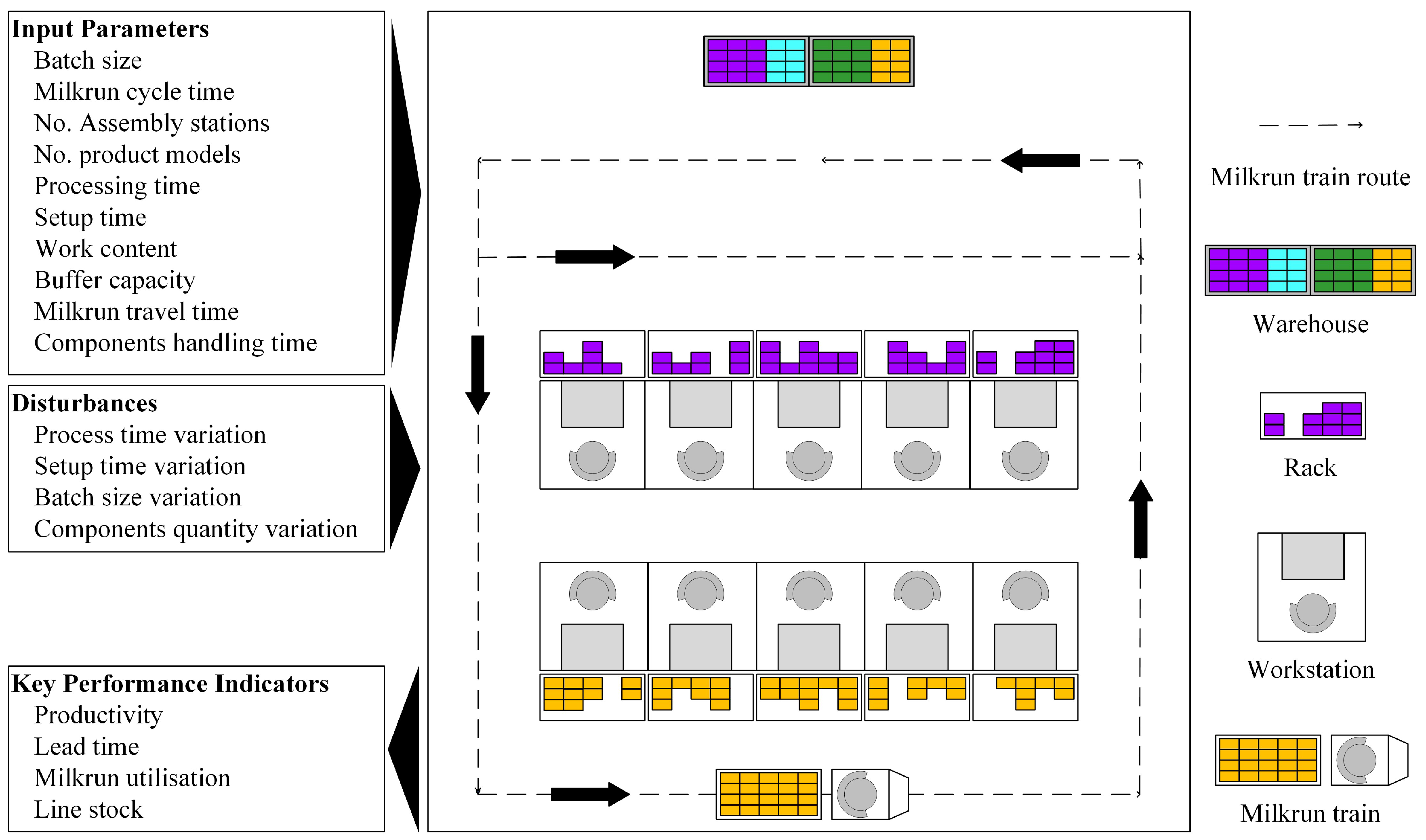
In this article, the operational performance of two assembly lines and the milkrun train that feeds them is evaluated under different conditions. The system consisting of assembly lines and internal logistics was studied by considering a set of inputs, a Discrete Events Simulation model and a set of output KPIs, as depicted in
Figure 1. The model consists of two main parts: the assembly lines and the supply chain feeding the components to the Assembly Line (AL) in containers using a milkrun train. Simulation was chosen for building this model because it allows the introduction of stochastic elements [
55], such as process or logistics variability, which is necessary to achieve this work’s goals. The simulation tool employed was FlexSim
® (2022.0, FlexSim Software Products, Inc., Orem, UT, USA). Several simulation scenarios are created by modifying different parameters and disturbances values to analyse desired aspects of the system behaviour.
Section 3.1 details the modelling assumptions.
Section 3.2 includes the notation and definitions employed, and
Section 3.3 includes the input data used in the models, which are used for validation (
Section 3.4) and the experiment design (
Section 3.5).
3.1. Assumptions
The simulation model depicted in
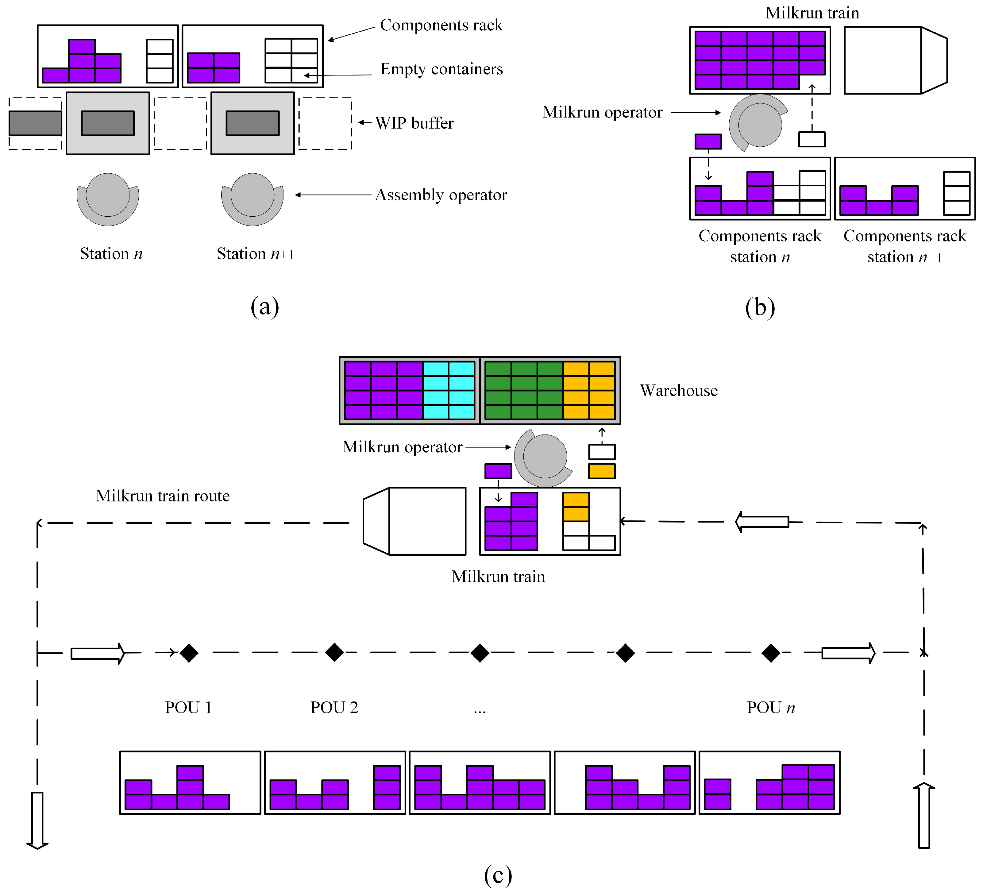
Figure 1 is made of two main subsystems: (1) two manual assembly lines, which feature operators, workstations, product buffers and components racks; and (2) internal logistics, which include a milkrun train, the components Points Of Use (POUs), a warehouse and the information flow necessary to ensure the assembly line receives the required components on time; see
Figure 2.
Assembly lines:
Figure 2a,b show the elements of the assembly lines used in this model, which feature the following assumptions following the classification of assembly systems by Boysen et al. [
6]:
The assembly systems are unpaced, buffered lines.
These are fixed-worker assembly lines: operators are assigned to stations.
There is manual assembly only (no semi- or fully automated work content).
The number of workstations is constant. Each station can process only one product unit at a time.
Operators need to gather all components specified by the Bill of Materials (BOM) to proceed to assemble at their stations; see
Figure 2a.
The demand mix is known and it continues for the whole simulation horizon.
The assembly lines can be single-model, mixed-model or multi-model. Single-model lines only produce one product variant per AL. Mixed-model lines can produce more than one model, but there is no setup time between products. Multi-model lines are similar to mixed-model lines but they do incur setup time losses when changing over from one product model to another.
Setup times, where present, are not dependent on the product sequence.
The product sequence consists of an alternating pattern of batches of products. The batch size is stochastic, based on a discrete uniform distribution to represent the probability of a batch being released to the assembly line with fewer units than standard. This represents the disturbances caused by upstream manufacturing processes. The probability distribution is governed by the batch size coefficient of variability ().
Processing and setup times are stochastic. They follow a lognormal distribution based on mean values and standard deviations, which are expressed by the coefficients of variability (, ).
Slightly different processing times on each station mean that these are unbalanced assembly lines, as shown in the ’Input’ subsection.
Internal Logistics:
Figure 2 shows the main components of the internal logistics, which consists of four subsystems:
Information flow between the assembly lines and the milkrun train, so that the milkrun picks up the right components for the product models that will be needed in the AL. This includes the calculations of the number of containers of each component
. This is worked out based on the expected consumption over the milkrun cycle time (
d), the no. of pieces of component
i per product unit (
) and the no. of pieces per container (
), with a minimum of 2, as shown in Equation (
1). This minimum of 2 containers is required to prevent assembly line starvation, which could occur otherwise since the milkrun logic implies taking empty containers and replacing them with full ones on the next cycle.
The number of pieces in each component container is stochastic, based on the standard number of pieces per container and a coefficient of variability (). A discrete uniform distribution is employed, which uses as the lower limit and the standard no. of pieces as the upper limit. This represents the probability of a certain number of pieces being non-conforming due to quality problems, inaccurate counting at the external suppliers’ production site or incorrect re-packing at the in-plant warehouse, especially for components packed in bulk, such as nuts and bolts.
Milkrun train picking at the warehouse (see
Figure 2c) is modelled as a single POU. The milkrun train is emptied upon arrival, and it is thereafter filled again with the required containers for the next supply cycle.
The milkrun transportation time from/to all POUs (
Figure 2c) is based on historical time measurements from the industrial study case. Since the data show very little variability, the model assumes a deterministic transportation time given by the input parameter
.
Supply chain operator loading and unloading of component containers to the assembly lines at each POU, as shown in
Figure 2b. There are two possible situations: (1) Regular cycle (same product model): the operator replaces the empty boxes in the ‘returns rack’ with full boxes of the same component. The handling time is different for full and empty containers; see the input subsection. (2) Product changeover cycle (before the assembly line changeover): in which the milkrun operator firstly replaces any current product empty container to ensure that the current batch can be finished and then loads the next containers of the next product components so that they are available to the assembly operators when they finish the stations’ changeover.
3.2. Notation
The following notations are introduced:
Input: Parameters
- Q
Batch size
-
Assembly cycle time
-
Milkrun cycle time
- L
No. of assembly lines, index l.
- K
No. of assembly workstations (no. POUs) per assembly line, index k.
- M
No. of product models, index m.
-
Processing time
-
Setup time
-
Work content (i.e., total process time)
-
No. of work in progress units between workstations
-
Milkrun transportation time to/from assembly line
-
Milkrun operator container handling time, empty container
-
Milkrun operator container handling time, full container
Input: Disturbances
-
Process time coefficient of variation:
-
Setup time coefficient of variation:
-
Conforming units per container coefficient of variation
-
Batch size coefficient of variation
Output: Key Performance Indicators
- P
Productivity (units/operator-h): production rate of conforming units per assembly operator.
-
Lead Time (min): average time for a batch of units to be finished from the moment the last unit of the previous batch is finished.
- U
Milkrun Utilisation (%): fraction of total available time that the supply chain operator is busy (picking components at the warehouse, driving the milkrun train and handling containers to load/unload the components at the POUs).
- S
Stock in the assembly line (units): average stock of components held in the assembly line measured in equivalent finished product units.
3.3. Input Data
The simulation model uses data provided by the industrial study case, which presents a common situation faced by plenty of manufacturing businesses globally.
Table 2 shows the model parameters base, min and max values.
The operations considered in this model include two manual assembly lines which assemble four product models, two on each line. The mean processing times for each model and station along with work content and cycle time is summarised in
Table 3. These processing times were obtained from the industrial company standard operating procedures, which in turn are calculated using MTM.
The products within a line share materials, technological features and general purposes, but they require different components, assembly fixtures and tooling. This calls for changeovers to adjust the workstations when a batch of a different product model is required. The parameter governing setup times is
, which takes each operator approximately 6 min (see
Table 2), independently of the product sequencing.
Each product unit consists of many different components, as shown in
Table 4. Most components are required only once per finished product unit, although some components, especially the smaller ones, may be required in larger numbers.
Components are transported to the POUs and then presented to the assembly operators in containers, i.e., boxes, trays or small trolleys. Each container carries a certain number of pieces of one component, typically a few dozens for middle- and large-size components, and about one hundred pieces for small components, such as bolts, screws and washers.
In this particular study case, an important number of components are packed in very large quantities per container compared to the number of pieces needed to feed the assembly line for the duration of the milkrun cycle. Note that the the milkrun cycle time is approximately similar to the time required to complete a production batch. To illustrate this fact,
Table 5 shows the number of components of each product model that are packed in
large quantities. Here,
large quantities refers to the case in which one single container includes a number of pieces allowing to assemble more than two full batches of products—i.e., it is equivalent to the assembly line consumption of two milkrun cycles.
When the milkrun operator arrives at each POU, the containers are handled between the train and the back side of the POU racks. Based on measurements at the industrial partner facility, one second was estimated for handling empty containers and two seconds for containers full of components, as shown in
Table 2. When walking from the milkrun train to the POU, the milkrun operator’s speed was considered 1 m/s. The milkrun train speed in the assembly line area was found to be around 1 m/s, and the POU positions are separated approximately 2 m from each other, resulting in a 12 m long assembly line. Regarding the milkrun train travel from the warehouse to either assembly line, the industrial partner measurements showed little variability for an average travel time of approximately 4 min each way. The milkrun preparation time at the warehouse (picking time) was simulated considering the warehouse as a single picking point and treated as any POU of the assembly line.
The DES model takes into account the inherent variability of manual assembly operations by using lognormal distributions for processing and setup times, following the recommendations of [
56]. The lognormal distribution is generated using the mean (
) values of
and
—see
Table 3—and the standard deviation (
), which is given as a percentage of the mean by the coefficients of variation
and
. The base values for the coefficients were estimated from historical data provided by the industrial partner of this study case. The data allowed estimating
and
to be in the range of 0.15–0.20 for manual assembly lines. Note that since one of the goals of this work is to analyse the influence of processing and setup times variability on the internal logistics performance,
and
will take a range of values in certain simulation scenarios. Another two sources of variability, introduced in
Section 3.1, are considered: the conforming units per container variability (
) and the batch size quantity variability (
). They are relevant along with the processing and setup variability because the logistic performance of the milkrun system is directly related to them.
3.4. Verification and Validation
The validation and verification of the simulation models were performed separately for assembly operations and internal logistics.
For the assembly operations section, historical production KPIs data were gathered and compared against the results of a simple parametric model and a discrete events simulation model. The results presented by the authors in [
57] allowed the validation of both models by comparison against real industry study case data. It was also possible to verify the parametric model against the simulation model (considering no variability) because their results difference was smaller than 3.5% for any considered performance metric. In summary, the results indicated that both parametric and simulation models slightly underestimate total output and that they overestimate the production rate, labour productivity and line productivity. Both models were found to be reliable for the context considered here since the mean relative error was 1.63% and the max relative error was 4.9%.
Regarding the internal logistics part of the simulation model, the validation was carried out using measurements at the industrial partner assembly lines from June 2022. A total of 18 milkrun cycle measurements were registered, finding an average milkrun utilisation of 78.4%. This was compared with the equivalent simulation model results (U = 71.6%) to calculate a relative error of 8.7%, slightly below 10%, which was considered satisfactory for the scope of this work.
3.5. Experiment Design
To address the research questions laid out in
Section 1, several simulation scenarios were designed and then implemented on the simulation model by modifying the model’s parameters.
Table 6 summarises the parameters and range of values used to set up the simulation scenarios.
The first research question—
‘(1) What is the effect on the operational and logistics KPIs of producing multiple models in an assembly line compared to single-model production? Are there significant differences between mixed-model and multi-model production from the milkrun internal logistics point of view?’—is examined by changing the number of product models under demand (one model per assembly line for single-model,
; two models per assembly line per mixed- and multi-model,
) and the setup time duration parameter (
set to 0 s for mixed-model, 480 s for multi-model). For this
scenario i., process and batch quantity coefficients of variability take their base values (
and
0.15,
0.10 ), and the conforming units per container coefficient of variability is set to 0, as stated in
Table 2.
The second research question—‘(2) How is the milkrun-assembly lines system affected by variability? In particular, to what extent is it impacted by assembly process variability and supply chain disturbances?’—will be decomposed into the three variability sources considered in the simulation model. Firstly, process variability is governed by parameters (assembly processing time variability) and (setup time variability). These parameters will take values ranging from 0 (no variability at all) up to 0.50 (high variability), making up scenario ii. Secondly, the batch size variability coefficient will be used to represent in-plant manufacturing issues leading to smaller-than-standard batches of products being released for assembly. Similarly to the previous scenario, in scenario iii. values will range from 0 to 0.50, covering from no disturbances up to half of the batches having fewer units than it was intended. Finally, scenario iv. looks into external supplier perturbations which are simulated using the components quantity coefficient of variability. will take values in the range of 0 to 0.20, meaning that each components container can have up to 20% fewer valid pieces in the less favourable case. The effect of the interactions between the variability parameters was not analysed because a preliminary two-level full factorial design of experiments showed that two-factor interactions were not significant for the KPIs under study in comparison to the effects of the variability parameters by themselves.
The following
Section 4 Results shows the outcome of the simulation scenarios introduced here.
4. Results
This section includes the outcome of the simulations corresponding to
scenarios i.-iv.
Section 4.1 addresses the first research question, and
Section 4.2 includes
scenarios ii.-iv., which jointly address the second research question.
The results shown here are obtained with a simulation horizon of 74 h with a warm-up time of 2 h (i.e., nine production shifts after the warm-up is finished). To account for the stochastic nature of the results, each simulation scenario is run 20 times. This number was chosen because it was found that using a larger number of runs did not affect the resulting output in a statistically significant manner. At the start of each simulation run, all assembly stations and buffers between them are empty as well as all the components racks and the milkrun train.
The results shown in this section are presented in boxplots where the upper and lower limit of the boxes corresponds to the first and third quartiles. The coloured line is the mean and the whiskers limits are set to 1.5 times the interquartile range. Outlier data points (beyond the whiskers) are marked by a circle. The charts scale has been kept constant across all simulation scenarios to facilitate comparison.
4.1. Single-Model vs. Mixed-Model, Multi-Model Assembly
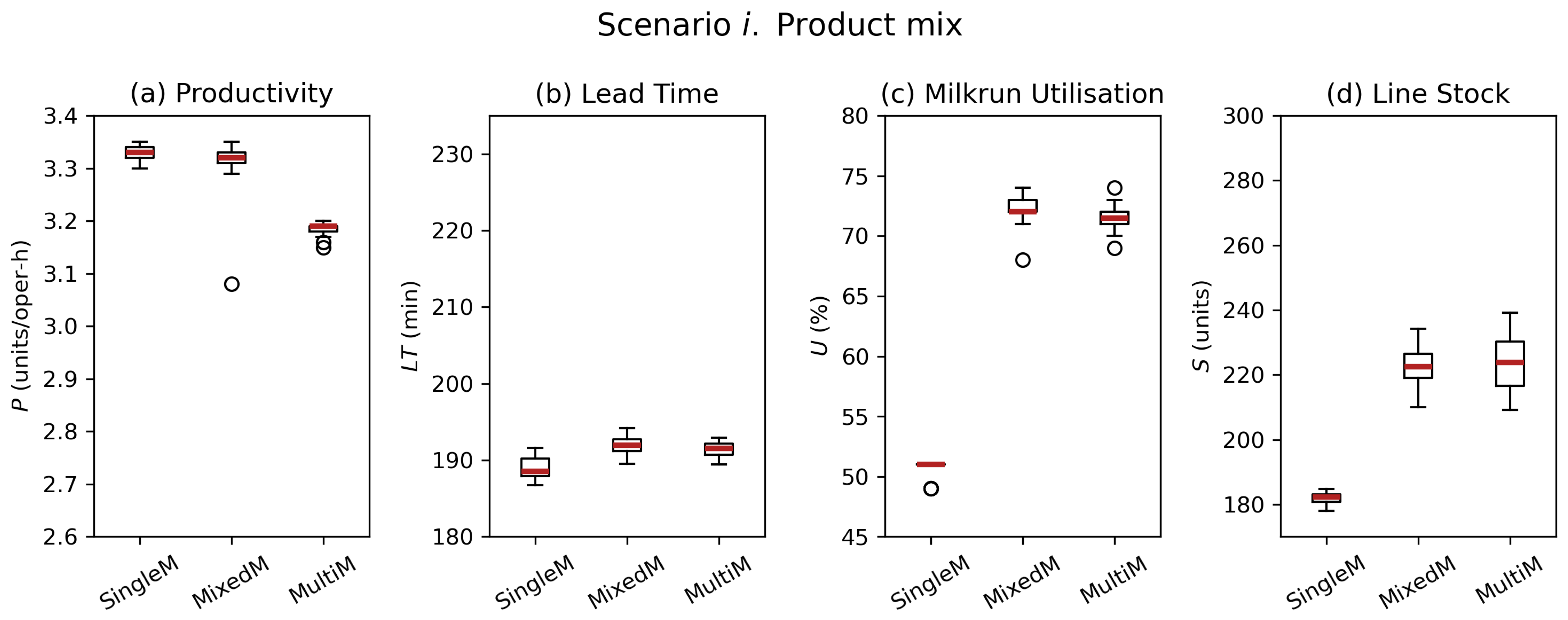
The selected operational KPIs comparing the performance of the assembly lines under
scenario i. demand conditions are shown in
Figure 3 and summarised in
Table 7.
The productivity of single- and mixed-model lines is significantly superior to multi-model lines, as is expected considering that the setup time becomes zero (from 480 s per batch of 48 units, which represents just below 5% of the time needed to complete the batch on average). The difference in productivity between single- and mixed-model lines is related to operator idle and blocked times following product model changeovers as a result of cycle time differences between the incoming and outgoing products. Said difference does not account for significant productivity results in this case. Batch lead time, as expected, is slightly larger for mixed- and multi-model lines compared to single-model lines.
On the internal logistics KPIs side, milkrun utilisation and assembly line stock show a clear differentiation between single-model assembly lines and the other two. Incorporating multiple product models increases greatly the utilisation (from 51% to 72%, a +44% increment). Note that this steep increase could be linked to the high percentage of components packed in large quantities. This will be examined in the next
Section 5 Discussion.
The component stock in the assembly line also suffers an increase for mixed- and multi-model lines driven by the same reason: single-model assembly lines see their average component stock decrease as the containers with very large quantities of pieces are consumed over time. Contrarily, mixed- and multi-model lines are constantly fed with small component boxes full of pieces. In the case shown here, the difference is significant but not dramatic, at an approx. +22% increase (from 182 to 223 units).
In summary, increasing product mix negatively affects operational KPIs (reduces productivity, increases batch lead time), which was expected. It also increases greatly supply chain operator utilisation (+44% rise), although the magnitude of this sharp increase could be attributed to the high percentage of components packed in large quantities.
4.2. Variability and Disturbances
This subsection looks at how increasing levels of variability affect the operational (
P,
) and internal logistics KPIs (
U,
S). As described in
Section 3.5, simulation experiments were set up to independently analyse the influence of assembly line process variability (
and
,
scenario ii.), batch size variability (
,
scenario iii.) and conforming components variability (
,
scenario iv.).
4.2.1. Process Variability
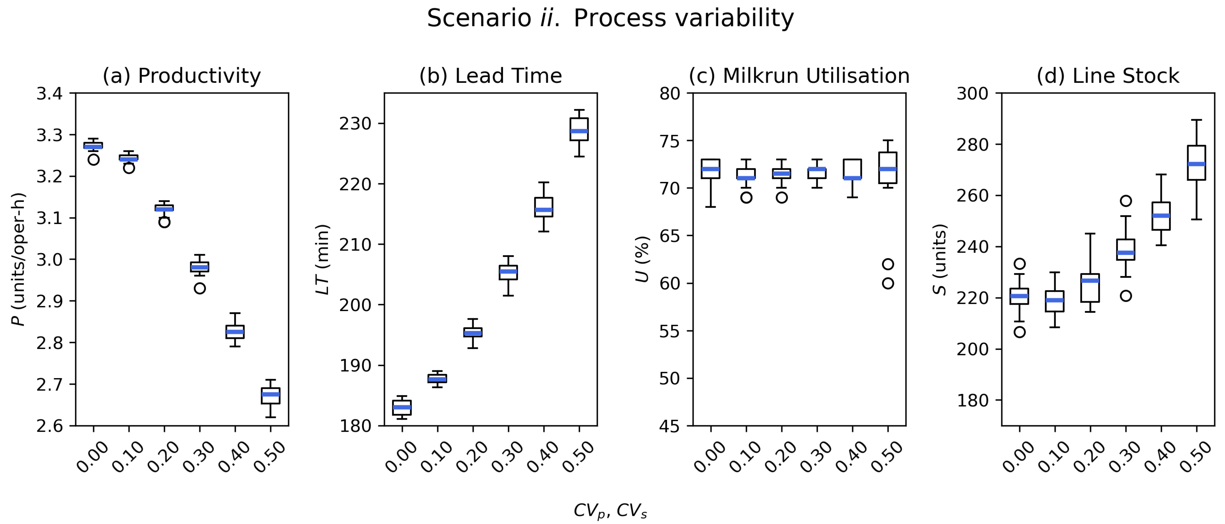
To analyse the impact of the assembly line process and setup variability, the respective coefficients were modified increasingly from 0 up to 0.50 (the base value for the industrial case study is 0.15; see
Table 2).
Figure 4 shows the results of this simulation scenario, and
Table 8 includes the results’ numeric values for average and standard deviation.
In terms of operational KPIs,
Figure 4a,b show that, as expected, an increase in process variability negatively the performance of the assembly line, especially considering that this lines’ number of work-in-process units is limited to one. In particular, it can be seen that the productivity deteriorates greatly when
and
are greater than 0.20 both in terms of mean and standard deviation. Batch lead time follows the same trend.
Figure 4c shows that
U does not suffer any changes, although its standard deviation increases slightly. On the other hand, the assembly line components’ stock levels are severely impacted, rising from approx. 220 units for none or very small variability (
and
at 0–0.10) up to an average of approx. 270 units for
0.50, which represents a noticeable +23% increase. Standard deviation also rises, but it remains small compared to the mean values of
S, as shown in
Figure 4d. In summary, only AL stock levels are affected by in-process variability, while the milkrun driver’s workload remains unaffected.
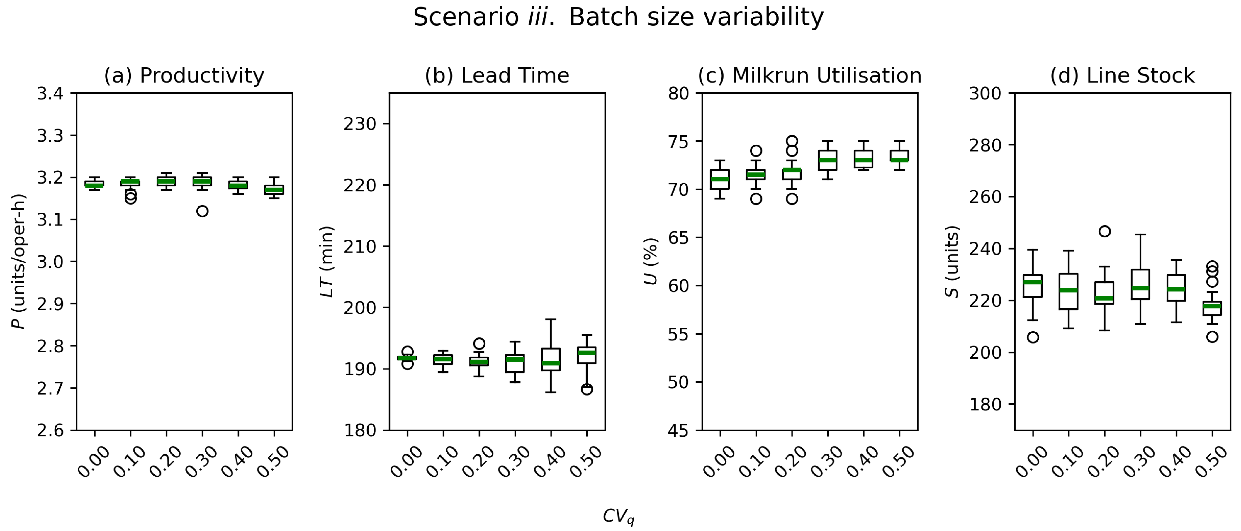
4.2.2. Batch Size Variability
To understand the impact that upstream manufacturing process issues would have on the assembly operational and internal logistics performance,
scenario iii. was set up by changing the value of
, which determines the probability of an assembly production batch smaller than standard.
takes values between 0 (no disruption) and 0.50 (meaning that on average, half the batches released to the assembly lines have between 36 and 48 units. The simulation results of
scenario iii. are summarised in
Figure 5, and average and standard deviation data are shown in
Table 9.
Figure 5a,b shows that the average of both line productivity and lead time remains constant despite changes in
. Although
P standard deviation increases slightly, it remains very low at about 0.25–0.43% of the average value. The lead time StDev, on the other hand, does increase more than five-fold while remaining very low compared to average values (StDev of 0.24–1.39%). Therefore, the data show that batch size variability has no significant impact on the operational KPIs. Although variability rises as
grows, it remains at very low levels in relative terms.
Figure 5c,d show very little impact on internal logistics KPIs as a result of an important rise in batch size variability. The milkrun utilisation average does increase slightly (from 71 to 73%, c.+4% rise), but the StDev reduction (from 1.25% to 0.82%) is not statistically significant. In a similar fashion, assembly line components stock decreases slightly in both average and standard deviation values, but none of these changes are statistically significant.
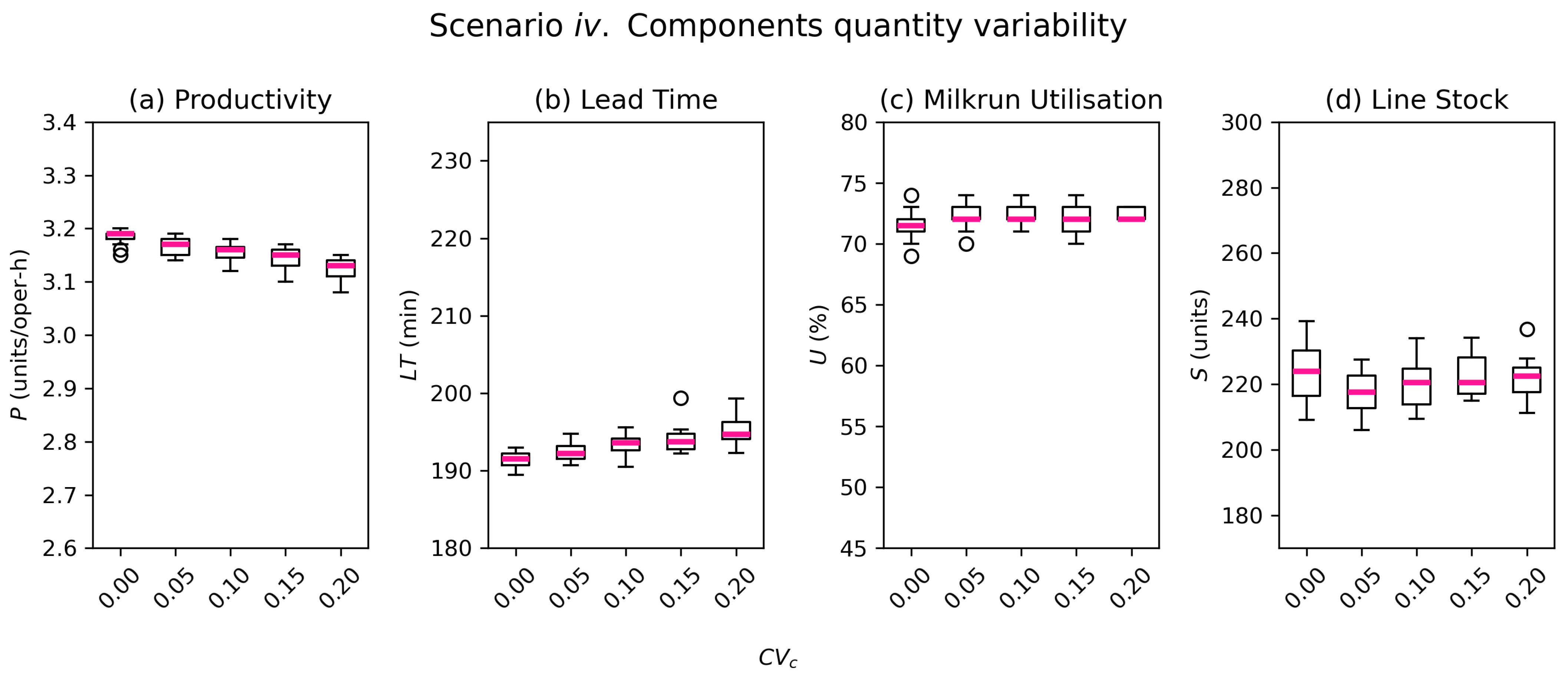
4.2.3. Components Quantity Variability
The goal of this subsection is to analyse the impact of the components quantity coefficient of variability
. This coefficient is employed to represent disturbances within in-house or external suppliers’ processes, resulting in a lower-than-standard number of conforming pieces in each component container. As explained in
Section 3, the number of conforming pieces per container is simulated using a discrete uniform distribution which has the inferior limit set to
percent of the nominal value.
Scenario iv. considers
values from 0 to 0.20, as shown in
Table 10.
Figure 6a shows that productivity is affected negatively by an increase in
, although the magnitude of the impact is very limited: only a −2.2% reduction from the base scenario when components containers have up to 20% less conforming pieces than expected. Similarly, lead time is impacted negatively by
increase, as depicted in
Figure 6b. The
average rises slightly (c.+2%) and suffers a greater dispersion of results (StDev increases by +54%). All in all, even a substantial increase in components quantity variability does not affect the assembly lines’ operational KPIs severely.
Regarding internal logistics KPIs,
Figure 6c,d show that an increase of
has no significant impact on either milkrun utilisation or assembly line component stock levels.
5. Discussion
The results shown in the previous section have been summarised in
Table 11.
Increasing the product mix from single- to mixed- and multi-model assembly lines results in a moderate impact on operational performance (P, ) but a very significant negative effect on internal logistics KPIs, which could have further implications. For instance, the rise of assembly line component stock would increase the required floor space and decrease the assembly line surface productivity.
It is important to note that according to the results shown in
Section 3.1, the greatest factor affecting
U is the product mix, with a remarkable +44% increase resulting from changing from single- to multi-model assembly.
This sharp increase in U is caused by the rising number of containers that need to be handled, which is due to two main reasons.
(1) First of all, the number of component containers to be handled is larger every time there is a product changeover, which is the case for almost every milkrun cycle under the assumption that the milkrun cycle time is approximately similar to the time required to complete a batch of products (cf.
in
Table 2 and
in
Table 3). The increased number of containers to be handled is due to the fact that the supply chain operator needs to take all the containers of the outgoing model from the POU racks regardless of how many component pieces are left and replace them with components for the incoming product model. During regular supply cycles, on the other hand, containers are only replaced if needed (empty boxes work as kanban signals).
(2) The second reason is related with the compound effects of the first reason and the fact that in this particular study case, we find a large number of components packed in large quantities (see
Table 5). This fact means that for a significant percentage of the components, each milkrun train carries enough pieces to assemble more than four times the required amount of pieces. Furthermore, the milkrun train will need to take back to the warehouse a full container and a half-empty container every time a changeover is needed.
Thus, it seems reasonable to conclude that milkrun utilisation is higher on mixed- and multi-model lines compared to single-model assembly lines. However, the magnitude of the increase shown in the Results must be considered carefully, since it it would be strongly related to the container quantities of this particular industrial study case.
As a closing remark on this subject, two aspects could be looked at in order to reduce the milkrun utilisation for multi-model assembly lines. Firstly, if enough shop-floor space is available, small components packed in large quantities could be left by the workstations, forming an assembly line supermarket, independent of the regular milkrun cycles. For larger components, relaxing the rule of minimum two containers (see Equation (
1)) could be considered. Secondly, packing components in smaller quantities (so that two containers cover approximately the consumption of a milkrun cycle) could also reduce the milkrun workload so that it is only slightly higher than for single-model assembly lines.
Production variability () is the most important disturbance factor affecting productivity, lead time and assembly line components stock. However, it does not affect supply chain operator utilisation because the productivity reduction implies a reduction of output rate (which slows down components consumption). The reason behind this is that the milkrun work logic establishes a fixed replenishment frequency (milkrun cycle time), resulting in a supply chain operator workload effectively unaffected by several minor variations over the course of a full replenishment cycle.
Despite the previous expectation that variability would always impact performance negatively, results from
Section 4.2.2 and
Section 4.2.3 show that the internal logistics KPIs are not sensitive to disturbances originated by batch size and components quantity variability (
and
respectively). This implies that employing milkruns for the internal logistics of flexible multi-model assembly lines under high-mix low-volume demand is a way to shield this part of the supply chain from upstream disturbances, arriving from either external or internal processes.
It was also found that variability regarding batch size (
) does not have any noticeable negative impact on operational performance, as shown in
Figure 5c.
Note that as mentioned in
Section 2, this article addresses a gap in the literature by specifically addressing in-plan logistics for multi-model assembly operations, including variability, and using a real study case—specially from an industry sector other than automotive.
The fact that the simulation model used in this work is based on a real industry study case provides valuable insight into the behaviour of similar assembly operations—internal logistics systems under increasingly hard conditions in terms of variability and product mix. However, it is important to note that this also limits the generalisation extent of the results obtained due to certain aspects listed below.
First of all, the case employed here considers only a relatively small product variation within each assembly line ( 13% and 34% for AL no.1 and AL no.2, respectively) and almost no difference in terms of average per model when comparing both lines ( c.2%). Understanding how much product variability affects the operational and internal logistics KPIs could be a potential avenue for further research to understand the extent of the potential benefits of employing milkruns for high-mix low-volume assembly.
Secondly, it could be argued that the number of conforming components coefficient of variability () only modifies the number of pieces per container available to the assembly operator, but it does not realistically capture the possibility of components actually arriving at the assembly line and then causing quality control failures or unexpected assembly process time increases, which would imply additional productivity losses due to reasons such as product rework and idle/blocked assembly operators.
Thirdly, milkrun transportation time was considered deterministic because the industry case measurements indicated this time were consistent. However, for multi-train production sites, variability caused by occasional milkrun train traffic jams could be considered.
Finally, modelling the milkrun train as a single wagon could be slightly underestimating its utilisation despite the satisfactory validation results. Specifically, in potential scenarios featuring longer milkrun cycle times—note that the parameter was unchanged through scenarios i. to iv.—this would entail a greater number of component containers and therefore potentially a greater number of required wagons leading to an increased walking time for the supply chain operator, which the current simulation model would not capture.
6. Conclusions
To address a mass customisation demand context that drives high-mix low-volume assembly operations, this article studied the implications of using milkrun trains for the internal logistics of multi-model assembly lines. Based on a real industrial study case from the white-goods sector, a discrete events simulation model was employed to set up four different scenarios which evaluate the effect of product mix and three different sources of variability. To measure such impact, a set of four Key Performance Indicators (KPIs) were used, two corresponding to assembly operations and two corresponding to supply chain efficiency.
It was found that multi-model lines increase significantly the milkrun utilisation and the assembly line components stock compared to single-model lines. However, the magnitude of this large increase could be partially attributed to particularities of the study case. Operational KPIs were also affected negatively but to a much lesser extent. Internal logistics performance is greatly affected by the variability of assembly line processing time, especially in terms of component stock. Other sources of variability, such as the ones affecting the number of units per production batch or the components quantity per container, have very limited impact on the selected KPIs. This would imply that employing milkruns for the internal logistics of flexible multi-model assembly lines under high-mix low-volume demand is a way to shield this part of the supply chain from upstream disturbances, arriving from either external or internal processes.
Two key limitations of this work are the relatively low product variability in terms of work content and the milkrun train physical features simplification.
Further research paths include exploring the implications of much greater product work content variability, incorporating more detailed physical models of the milkrun train and expanding the simulation model to include adjacent layers that could constrain the performance of the assembly system as a whole, such as quality (defects, reworks, quality controls) or breakdowns and maintenance.


 ,
, 


