Article

Optimal Design of High-Speed Electric Machines for Electric Vehicles: A Case Study of 100 kW V-Shaped Interior PMSM

1
SATIE, CNRS, ENS Paris-Saclay, Paris-Saclay University, 4 Avenue des Sciences, 91190 Gif-sur-Yvette, France
2
Stellantis, Route de Gisy, 78140 Vélizy, France
3
SATIE, CNRS, CY Cergy Paris University, 33 Bd du Port, 95000 Cergy, France
4
LMPS, CNRS, ENS Paris-Saclay, Paris-Saclay University, 4 Avenue des Sciences, 91190 Gif-sur-Yvette, France
5
Stellantis, 212 Bd Pelletier, 78955 Carrières-sous-Poissy, France
*
Author to whom correspondence should be addressed.
Machines 2023, 11(1), 57; https://doi.org/10.3390/machines11010057
Submission received: 29 November 2022 / Revised: 27 December 2022 / Accepted: 27 December 2022 / Published: 3 January 2023
(This article belongs to the Special Issue Optimal Design of a High-Speed Motor)

Abstract

:
The need of compact machines increased in recent years due to increases in raw materials’ price. Hence, many studies are currently being conducted on high-speed challenges to propose an optimal design methodology. AC losses in windings are often not included in the optimization process and are treated in post-processing by choosing a suitable conductor’s diameter to mitigate skin and proximity effects. This paper presents an optimization and design methodology for high-speed electric machines considering these losses, using models with an interesting trade-off between computation time and accuracy, which is helpful for large-scale optimization, in which more than 9,600,000 machines are evaluated. Optimizations are conducted on 100 kW high-speed one-layer V-shaped interior permanent magnet synchronous machines, widely used in vehicles thanks to their high power density, based on the specifications of the Peugeot e208, for different values of pole pairs and maximum speed. The influence of lamination thickness, fill factor, and maximum current density on the optimal design is also investigated. This paper concludes the utility of increasing speed to achieve high power density and proposes best alternatives regarding automotive constraints. Results show that the number of pole pairs is not always a key parameter in obtaining the lowest volume, especially at high speed.

1. Introduction

The need for high-speed electric machines has seen rapid growth in recent years due to their numerous advantages in terms of mass and volume reduction and hence cost reduction. However, new phenomena appear at high-speed and need to be studied and considered during the design process. Many works have been done to determine challenges related to high-speed machines [1,2,3,4]. One of the main challenges is the mechanical constraints of the rotor. The maximum rotational speed should be designed to guarantee the mechanical integrity of the rotor. Another challenge is high-frequency phenomena that lead to significant losses at high-speed, which can cause damage to the machine if not well designed. Losses occurring in the machine have been studied and can be listed as follows: iron losses, permanent magnet losses, mechanical losses, and winding losses. At high speed, the latter, known as AC losses in windings, has recently received increased attention. At low speed, they are evaluated based on the Joule effect only; however, at high-speed, new effects known as the skin effect, proximity effect, and circulating currents appear and need to be considered.
Many works were conducted on the design and optimization of high-speed machines [5,6]. Reference [7] proposes topology modification of a flat inserted permanent magnet synchronous machine (PMSM) based on magnet segmentation to ensure a maximum rotational speed of 35,000 rpm. Geometric modifications of the rotor are also proposed in [8,9] to improve performances of the V-shaped interior PMSM (IPMSM) for vehicle application. Different machine’s topologies have been compared to select the suitable one for electric vehicle application [10] and high-speed application [11]. The results showed that a single-layer V-shaped IPMSM was the best candidate that respects automotive constraints. Both single- and double-layer V-shaped IPMSM with high fill factor and high maximum current density are good candidates for high-speed application. A multiphysics design and optimization methodology of single-layer V-shaped IPMSM for automotive applications based on metamodels was proposed in [12]. Surface-mounted PMSM (SM-PMSM) have also received interest for high-speed application due to their mechanical integrity, which can be satisfied with a sleeve. A multiphysics design and an optimization methodology of high-speed SM-PMSM for EV application based on 2D analytical models were proposed in [13]. However, in these works, high-frequency losses in windings were not included in the design and optimization process. AC losses in windings are often treated during post-processing by choosing a suitable conductor’s diameter to reduce high-frequency effects. At high-speed, this method could not be efficient. Consequently, the design and optimization process should include AC losses in windings. Three main models in the literature exist to evaluate losses due to the three high-frequency effects in windings mentioned above: analytical, finite element, and hybrid models. A multi-objective design optimization of SM-PMSM for automotive application, considering skin and proximity effects using analytical models, was proposed in [14]. Analytical models [15,16] have the great advantage of rapid computation time but lack precision and cannot be applied to complex rotor geometries. Contrarily, finite element models [17] are accurate but time-consuming, preventing their use for large-scale optimization. Hybrid models [18,19] are a good compromise between these two models. They can be applicable to any geometry and allow lower computation time than analytical models. A hybrid model for AC losses in windings was proposed in [18,19], which can be integrated into the optimization process by guaranteeing an exciting trade-off between accuracy and computation time.
Iron losses represent a noticeable part of losses in the machine, especially at high-speed. New manufacturing technologies have been proposed to produce laminations with lower thickness [20], which is essential in reducing iron losses at high-speed. Other parameters are worth studying for high-speed machines. Comparisons conducted on different machines in [11] showed that maximum current density and slot fill factor were two advantageous parameters for high speed. Increasing these parameters allows increased power and torque density. New adapted cooling methods [
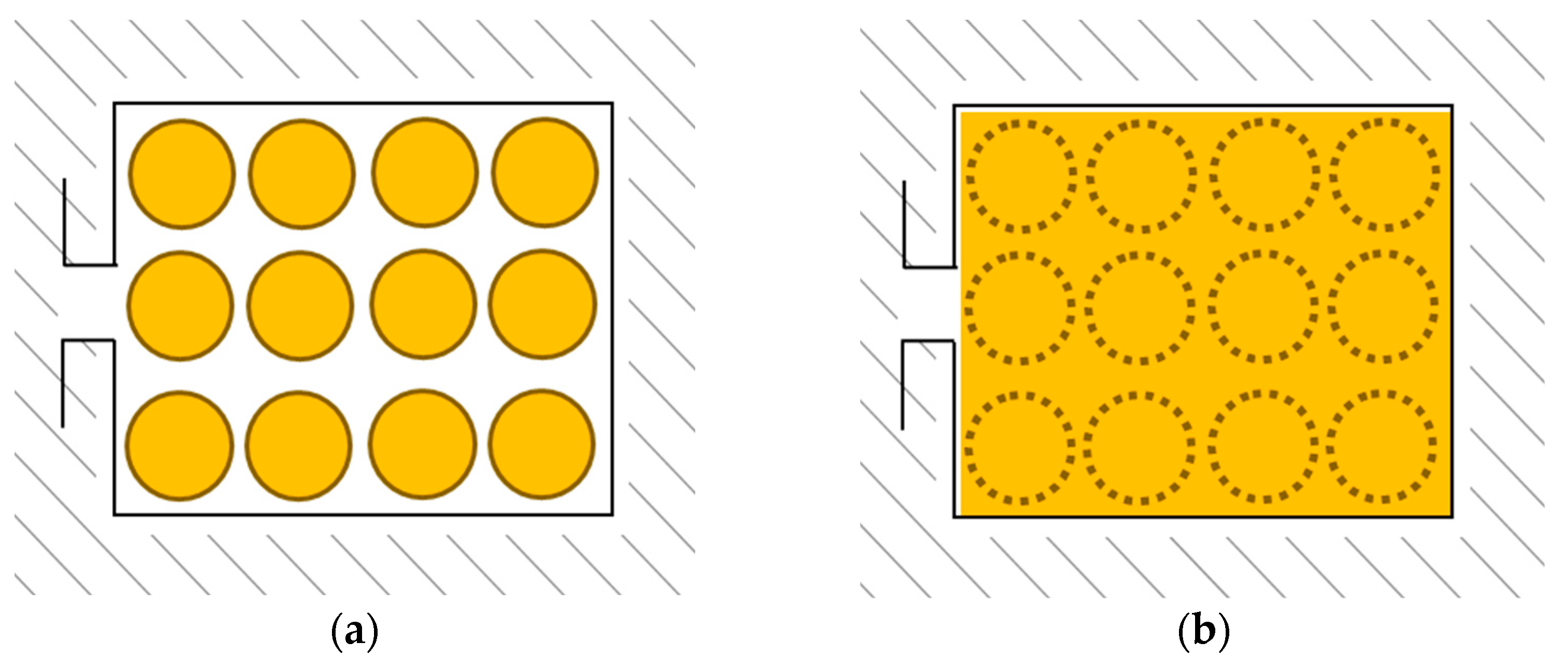
21] have been used to guarantee a high value of maximum current density. For conductors with a circular shape, a high fill factor can be achieved using die-compressed windings [22]. However, increasing maximum current density and fill factor can considerably increase the proximity effect between conductors. Hence, the influence of these parameters (lamination thickness, maximum current density, and fill factor) on the performances of the optimal design of high-speed machines is studied in this paper. By improving these three parameters, this will allow determining the best achievable performances of high-speed machines in terms of power density.
V-shaped IPMSM is the most widely used in electric vehicles among all types of synchronous machines due to its high power density. The electric vehicle Peugeot e208 is equipped with this machine, with a maximum rotational speed of 14,000 rpm. Tesla also uses this type of machine for its electric vehicle Tesla M3 with a maximum rotational speed of 20,000 rpm, which is currently the highest one used in the automotive industry. AVL [23] has designed and prototyped this machine for electric vehicle application, with the maximum rotational speed achieving 30,000 rpm. This paper aims to evaluate the utility of high-speed machines for electric vehicles and determines up to what speed it is worthwhile for automotive application. For this purpose, V-shaped IPMSM is selected for this study since it is of great interest. The machine will be optimized, based on specifications of the Peugeot e208, for four different values of maximum rotational speed: 15,000 rpm, 20,000 rpm, 30,000 rpm, and 40,000 rpm. In this work, more than 9,000,000 machines were evaluated during the optimization process. To evaluate the machine’s performances, we will use the design methodology of the V-shaped IPMSM described in [24]. However, since high-frequency losses in windings are not considered, an adapted optimization methodology, including hybrid models of AC losses in windings, is defined. The new optimization methodology is presented in this paper.
Section 2 presents the different definitions of high-speed machines in the literature. The methodology of the design and optimization of high-speed machines is described in Section 3. Section 4 presents the optimization specifications for an electric vehicle. Finally, optimization results and conclusions are presented in Section 5.

2. Definitions of High-Speed Machines

The notion of high speed is not only linked to a high rotational speed. Two electric machines with the same rotational speed but different outer rotor radii have different peripheral speeds; therefore, they may have various design constraints.
There is no unique definition of a high-speed electric machine in the literature. Multiple definitions of high-speed electric machines proposed by researchers are summarized in Table 1. Definition 1 characterizes qualitatively high-speed electric machines, whereas other definitions are based on quantified formulas. Definitions 2 and 3 are based on the rotor peripheral speed V p . Definition 4 is based on the notion of guide number [25] D Ω = Ω ( rpm ) × P ( kW ) , which is broadly used for high-speed electric machines in the literature [26,27].

3. Methodology of Design and Optimization of High-Speed Machines

The studied electric machine is an internal permanent magnet synchronous machine (PMSM). Permanent magnets (PM) are inserted in the rotor in a V shape, as shown in Figure 1. The rotor can contain multiple layers of magnets, but in the context of this work, we are only interested in the rotor with one layer of magnets. This machine is used in most electric and hybrid vehicles due to its high power density. The stator and rotor of the machine are geometrically modeled in [24]. The geometric parameters of a one-layer V-shaped IPMSM are listed in Table 2. The air gap length is a fixed parameter; hence, the number of geometric parameters of the stator and the rotor is 7 and 11, respectively, to which the active length of the machine is added. Therefore, the total number of the geometric parameters of the machine is 19. To these geometric parameters are added the excitation parameters for each operating point P i : current density and control angle. These will be discussed later in the section on optimization methodology.

3.1. Design Methodology of High-Speed Machines

In this section, the design methodology of high-speed machines is presented. First, the evaluation methodology of both electromagnetic and mechanical performances is presented. Then, models of losses occurring in the machine accounting for high-frequency phenomena are presented.

3.1.1. Electromagnetic and Mechanical Modelling

The electromagnetic performances of the machine are evaluated using a 2D finite element model. Simulations are performed using an Open Source XFEMM® integrated into Matlab®. The electromagnetic performances of the machine are performed using magneto-static evaluations at each angular position of the rotor, which reduces computation time. The latter can be reduced further by using mechanical and electrical symmetries of the machine, which makes it possible to launch the simulations on only one pole of the machine and 1⁄6 of the electrical period. Electromagnetic quantities are reconstructed based on these symmetries, as detailed in [24]. The machine has three phases and is supplied with sinusoidal current using an ABC model. Two variables are defined for each operating point: current density and control angle. The former allows defining ampere-turns based on the required fill factor and slot area. Hence, the number of winding turns is not previously known but is determined downstream of the simulations according to the evaluated induced voltage and maximum DC voltage [24].
The main objective of increasing the rotational speed is to obtain compact machines. The machine’s volume reduction must be done while guaranteeing the mechanical integrity of the rotor. Thin magnetic bridges allow the field lines to be conducted towards the air gap but negatively influence the rotor’s mechanical strength. Thus, evaluating the mechanical strength of the rotor is essential, especially for high-speed machines. The rotor is optimized by acting mainly, in the case of the studied machine, on dimensions of PM, air holes, and magnetic bridges separating the two magnets. Mechanical stresses are evaluated using a hybrid linear 2D model [24] combining the analytical method “the equivalent ring method” and finite element simulations performed using Matlab’s PDE Toolbox.

3.1.2. Losses Modeling

FEMM considers only low-speed phenomena. Hence, losses due to high-speed phenomena need to be modeled. Losses occurring in the machine are presented below, as is their model.
  • Iron losses:
Iron losses in the machine increase considerably at high frequency. The losses consist of three components: hysteresis losses, eddy current losses, and excess losses. Volumetric iron losses for a sinusoidal magnetic field are evaluated using the Berttoti model [30]:
P F e r = k h y s t f B m 2 + k e d d y 1 T 0 T ( d B d t ) 2 d t + k e x c 1 T 0 T | d B d t | 1.5 d t
where f is the frequency; B m is the magnetic field; and k h y s t , k e d d y , and k e x c are coefficients of hysteresis losses, eddy currents losses, and excess losses, respectively. This formula is applied to both the magnetic field’s radial and tangential components. This formula is applicable to a magnetic field with a sinusoidal waveform. However, for an arbitrary waveform, losses are evaluated by summing losses due to each harmonic, which can be obtained using Fourier series decomposition. This formula is applied at the level of each mesh using the magnetic field value obtained with simulations.
  • PM Losses:
Although the losses in the magnets are very low compared to the total losses in the machine, they must be evaluated to avoid damaging magnets, such as their demagnetization due to the increase in temperature. The instantaneous losses in each magnet are expressed using the following formula [31]:
P P M ( t ) = l a c t σ P M i = 1 N i J P M , i 2 ( t ) . S i
where σ P M is the conductivity of the magnets, N i is the number of meshes in the magnet, S i is the area of each mesh i in the magnet, and J P M , i is the current density value in the mesh i of the magnet expressed as follows:
J P M , i ( t ) = σ P M . [ A z , i t 1 S P M i = 1 N i A z , i t S i ]
where S P M is the area of the magnet, and A z , i is the vector potential evaluated at the mesh i and at each instant.
  • Mechanical Losses:
At high speed, mechanical losses increase and represent a significant part of total losses; hence, they must be accounted for during the design process. These losses consist of bearing and windage losses [32]:
P m e c h = P b e a r i n g s + P w i n d a g e
Bearing losses are due to friction and depend on factors such as lubricant, type of bearings, rotational speed, pressure, and the load of the bearing. They are accessible by measurements and can be estimated by the following formula:
P b e a r i n g s = 0.5 Ω μ F D b e a r i n g
where Ω is the rotational speed, μ is the friction coefficient, F is the load applied on bearings, and D b e a r i n g is the inner diameter of the bearings.
Windage losses consist of air gap losses P w i n d a g e , 1 and the losses at the end surfaces of the rotor P w i n d a g e , 2 :
P w i n d a g e = P w i n d a g e , 1 + P w i n d a g e , 2
The losses at the level of the air gap are expressed as follows:
P w i n d a g e , 1 = 1 32 k C M π ρ D o u t , r 4 l a c t Ω 3
where k is the roughness coefficient representing the smoothness of surfaces of both the stator and the rotor, C M is the torque coefficient, ρ is the density of the fluid flowing through the air gap, and D o u t , r is the outer rotor diameter. The coefficient k is equal to 1 in our study. The coefficient C M depends on the value of the Couette Reynolds number R e δ = ρ . Ω . R o u t , r . δ μ , where μ is the dynamic viscosity of the fluid flowing through the air gap. The coefficient C M is expressed as follows:
C M = 10 ( 2 δ / D o u t , r ) 0.3 R e δ       R e δ < 64 C M = 2 ( 2 δ / D o u t , r ) 0.3 R e δ 0.6       64 < R e δ < 5.10 2 C M = 1.03 ( 2 δ / D o u t , r ) 0.3 R e δ 0.5       5.10 2 < R e δ < 10 4 C M = 0.065 ( 2 δ / D o u t , r ) 0.3 R e δ 0.2       10 4 < R e δ
The losses at the end surfaces of the rotor are expressed as follows:
P w i n d a g e , 2 = 1 64 C M ρ Ω 3 ( D o u t , r 5 D i n n , r 5 )
where D i n n , r is the inner diameter of the rotor, and C M is the torque coefficient. The latter is expressed as a function of the tip Reynolds number R e r = ρ Ω D i n n , r 2 μ as follows:
C M = 3.87 R e r 0.5       R e r < 3.10 5 C M = 0.146 R e r 0.2       R e r > 3.10 5
  • Winding losses:
Winding losses have usually been assumed to be induced by the Joule effect only. However, this effect represents only DC losses in windings, which is available for low-frequency design. Therefore, high-frequency phenomena in windings must be considered when designing high-speed electric machines. These phenomena are the skin effect, proximity effect, and circulating currents effect appearing in the case of parallel strands. In our study, only skin and proximity effects were considered. Circulating currents are not integrated into the design and optimization process since this effect strongly depends on the locations of the multiple strands, which are random in the case of circular wires. Therefore, this effect is not considered during the optimization process but can be studied during post-processing.
Skin effect losses, also called strand-level skin effect losses, in a conductor with a circular shape are formulated based on an equivalent resistance called skin resistance, as follows:
P s k i n = R s k i n I R M S 2
where I R M S is the RMS value of the current, and R s k i n is the skin resistance expressed as follows [33]:
R s k i n R D C = γ 2 . b e r 0 ( γ ) b e i 0 ( γ ) b e i 0 ( γ ) b e r 0 ( γ ) b e r 0 2 ( γ ) + b e i 0 2 ( γ )
where
γ = d δ . 2 δ = 1 π f μ 0 σ R D C = l σ S b e r n ( x ) = R e ( J n ( x . e j . 3 π 4 ) ) b e i n ( x ) = I m ( J n ( x . e j . 3 π 4 ) ) b e r 0 ( x ) = b e r 1 ( x ) + b e i 1 ( x ) 2 b e i 0 ( x ) = b e r 1 ( x ) + b e i 1 ( x ) 2
where γ is a dimensionless parameter, d is the conductor’s diameter, δ is the skin depth, R D C is the DC resistance, l is the conductor’s length, σ is the conductor’s conductivity, b e r n and b e i n are Kelvin functions of order n , b e r n and b e i n are the derivative of the Kelvin functions of order n , J n is the Bessel function of order n , and j is the imaginary unit ( j 2 = 1 ).
Proximity effect losses, also called strand-level proximity effect losses, in the case of a conductor with a circular shape, are expressed as follows [34]:
P p r o x i m i t y = 1 T 0 T π l σ d 4 64 ( d B d t ) 2 d t
where T = 1 / f is the electrical period, and B is the magnetic field flowing through the conductor.
This formula is applied for each conductor based on the magnetic field flowing through it that can have an arbitrary waveform. In the case of a conductor with a circular shape, proximity effect losses can be evaluated without using radial and tangential components of the magnetic field since the conductor’s cross-section shape is the same on both axes. However, in the case of a conductor with a rectangular shape, proximity effect losses must be evaluated separately for each component [35].
Two methodologies are proposed in the literature to evaluate proximity effect losses [36,37]: detailed finite element analysis (DFEA) and simple finite element analysis (SFEA). DFEA requires drawing the conductors inside the slot and using a fine mesh to evaluate the magnetic field. In contrast, SFEA assumes a slot uniformly filled with conductor material, which allows using a coarse mesh. The latter has the great advantage of reduced computation time, making it suitable for large-scale optimization. Figure 2a shows a slot filled with conductors used for DFEA. Figure 2b shows its equivalent slot uniformly filled with conductor material and virtually placed conductors used for SFEA. DFEA and SFEA models are equivalent when the slot is uniformly and entirely filled, and ampere-turns are the same.
Losses due to both skin and proximity effects are evaluated separately. Total winding losses can be obtained using the orthogonality principle [38], which allows summing both losses under the assumption of a uniform magnetic field flowing through the conductor. Hence, winding losses are expressed as follows:
P w i n d i n g = P s k i n + P p r o x i m i t y

3.2. Optimization Methodology of High-Speed Machines

In this section, we will present a new optimization methodology based on the one presented in [24], accounting for both skin and proximity effects during the optimization process.
Evaluating high-frequency losses in conductors requires the knowledge of the number of conductors, their diameter, and their locations in the slot. However, as mentioned in the previous section, the number of conductors is not known upstream of the simulation but is determined based on voltage constraint. Hence, we will propose the following methodology to evaluate the AC losses.
First, the geometric parameters of the electric machine and supply parameters at each operating point are determined. Skin depth is then evaluated based on the frequency value for each operating point.
Next, we will create a virtual 2D grid covering the slot as shown in Figure 3, where the pitches d x and d y along the x- and y-axes, respectively, are taken as equal to the lowest skin depth evaluated previously.
For each operating point, the magnetic field’s value at each node j of the grid is stored at each instant. Once the simulations are performed, the number of turns is determined based on the voltage constraint. It corresponds to the number of turns for one phase in each slot. Each turn corresponds to a bundle, which is composed of several strands connected in parallel. The number of strands in parallel (also called n.s.h.: number of strands in hand), their diameter, and their locations are essential for evaluating AC losses. Therefore, we are going to study several configurations of n.s.h. and strand’s diameter by virtually placing them in the slot, as shown in Figure 4b for the DFEA model to have equivalence with the SFEA model shown in (Figure 4a). This equivalence is guaranteed by respecting the following three conditions:
  • The distance between the strands must be guaranteed in order to take into account the thickness of the insulation,
  • The slot must be uniformly and completely filled,
  • The required fill factor must be verified.
The studied strand’s diameter ranges from 0.6 mm to 1 mm. Only manufactured values of strand diameter in this range are investigated. The studied n.s.h. ranges from 1 to 100. All values of n.s.h. and strand diameter are checked, and only feasible winding configurations that satisfy the three conditions above are selected. These three conditions allow realistic windings similar to those used in real electrical machines [39].
For each winding configuration (n.s.h. and strand’s diameter), the location of each strand is known thanks to its virtual location. The closest grid’s node to the center of each virtual strand is determined, as shown in Figure 5.
For each winding configuration, proximity effect losses are evaluated for each strand based on the magnetic field value stored during simulations at its closest grid’s node, as mentioned above, using SFEA model and Formula (14). Skin effect losses are also evaluated based on the strand’s diameter and frequency using Formula (12). Among all feasible winding configurations, the one with the lowest total winding losses is selected. Hence, in addition to the geometry of the electric machine and its excitation parameters, the optimization also proposes a winding configuration, which is the number of strands in hand, the strand’s diameter, and the strands’ locations in the slot. Designing the machine for a given driving cycle using finite element models requires very high computation time. Therefore, the number of operating points is reduced as proposed in [11,24]. In this work, as shown in Figure 6, electric machine performances are evaluated for two operating points P 1 and P 2 . The optimization is conducted using genetic algorithm (NSGAIII) with three objectives:
  • Objective 1: Mass of the machine,
  • Objective 2: Total losses at Point P 1 ,
  • Objective 3: Total losses at Point P 2 .
The optimization methodology is summarized in the following flowchart (Figure 7):

4. Specifications

In this section, we will present the required specifications, similar to the performances of the machine used in the electric vehicle Peugeot e208. Table 3 lists all the required specifications. Optimizations are performed for two operating points (Figure 6). The electric machine is optimized for four different maximum rotational speeds and three different numbers of pole pairs. This allows determining the optimal number of pole pairs of V-shaped IPMSM at each maximum rotational speed for transport application. Required torque at both operating points depends on the maximum rotational speed. Its value at points P 1 and P 2 is expressed as follows:
T P 2   ( N . m ) = P m a x ( W ) Ω m a x ( r a d / s ) T P 1   ( N . m ) = T P 2 ( N . m ) k Ω
Many works in the literature [11,21] show the utility of using advanced technologies and high-speed to increase power density. Obtained results in [11] show that it is essential to increase both fill factor and maximum current density to achieve meaningful results in terms of power density for high-speed machines. The achieved fill factor is usually 45% for conductors with a circular shape, which is lower than hairpin windings composed of conductors with a rectangular shape that can achieve a fill factor of 65%. Increasing the fill factor for circular conductors requires advanced technologies, such as die-compressed windings [22]. Maximum current density can also be improved using advanced cooling methods [21]. Another parameter that is also worth studying is lamination thickness, which is directly affecting iron losses. These losses can be reduced by privileging thinner laminations. Manufacturers currently use these new technologies to achieve high power and torque density. For example, in order to achieve high torque density, the automotive company Tesla uses thinner laminations (0.25 mm) and a high maximum current density (33.7 Arms/mm²) in the electric machine used for its vehicle Tesla M3.
Optimizations are conducted for classic and new technologies to determine the utility of these new technologies at high speed. Table 4 presents details of each type. For each technology type, 12 optimizations are conducted. Each optimization concerns one value of maximum rotational speed and one value of pole pairs. Hence, the total number of optimizations to be conducted is 24.

5. Results

In this section, we are going to present, in the first step, the optimization results for each maximum rotational speed. Then, important conclusions and comparisons of optimal electric machines are presented. We define the following notations:
-
P v o l : Power density (kW/L);
-
P M / P : Quantity of magnets per power (g/kW);
-
C o p p / P : Quantity of copper per power (g/kW);
-
R o u t s : Outer radii of stator (mm);
-
L a c t : Active length of the machine (mm);
-
DSW: Distributed stranded winding;
-
DHW: Distributed hairpin winding;
-
I 1 ,   I 2 : RMS value of current per phase at points 1 and 2 (Arms);
-
J 1 ,   J 2 : Current density at points 1 and 2 (Arms/mm²);
-
N t u r n s : Number of turns per coil;
-
R p h : Resistance per phase ( m Ω );
-
n s h : Number of strands in hand;
-
d s h : diameter of strand (mm);
-
η 1 ,   η 2 : Efficiency at points 1 and 2 (%);
-
P J 1 ,   P J 2 : Joules losses at points 1 and 2 (W);
-
P I 1 ,   P I 2 : Iron losses at points 1 and 2 (W);
-
P A C 1 ,   P A C 2 : AC losses at points 1 and 2 (W);
-
P M 1 ,   P M 2 : Mechanical losses at points 1 and 2 (W);
-
C T : Classic technologies;
-
N T : New technologies;
-
M Ω m a x ( k . t r / m i n ) p C T : Optimized electric machines using classic technologies with p pole pairs and operating at maximum speed Ω m a x ( k . r p m ) ;
-
M Ω m a x ( k . t r / m i n ) p N T : Optimized electric machines using new technologies with p pole pairs and operating at maximum speed Ω m a x ( k . r p m ) ;
-
M Ω m a x ( k . t r / m i n ) p C T * : Electric machine with highest power density using classic technologies with p pole pairs and operating at maximum speed Ω m a x ( k . t r / m i n ) ;
-
M Ω m a x ( k . t r / m i n ) p N T * : Electric machine with highest power density using new technologies with p pole pairs and operating at maximum speed Ω m a x ( k . t r / m i n ) .
Each optimization corresponds to a given value of pole pairs, maximum rotational speed, and technology type. We have an initial population of 400 individuals and 1200 generations, considering all the restarts to reach convergence at the Pareto front, representing 400,800 evaluated machines for each optimization. By combining the 24 optimizations corresponding to all the pole pair values, all the maximum rotational speed values, and the two types of technologies, we obtain 9,619,200 (=24 × 400,800) evaluated machines. To do this, we used two powerful computers: Intel® Xeon® X5690 3.47 GHz processor with 160 cores and AMD Ryzen™ Threadripper™ 3970X processor with 32 cores. All of these optimizations lasted 6 months.

5.1. Maximum Rotation Speed Ω m a x = 15,000 rpm

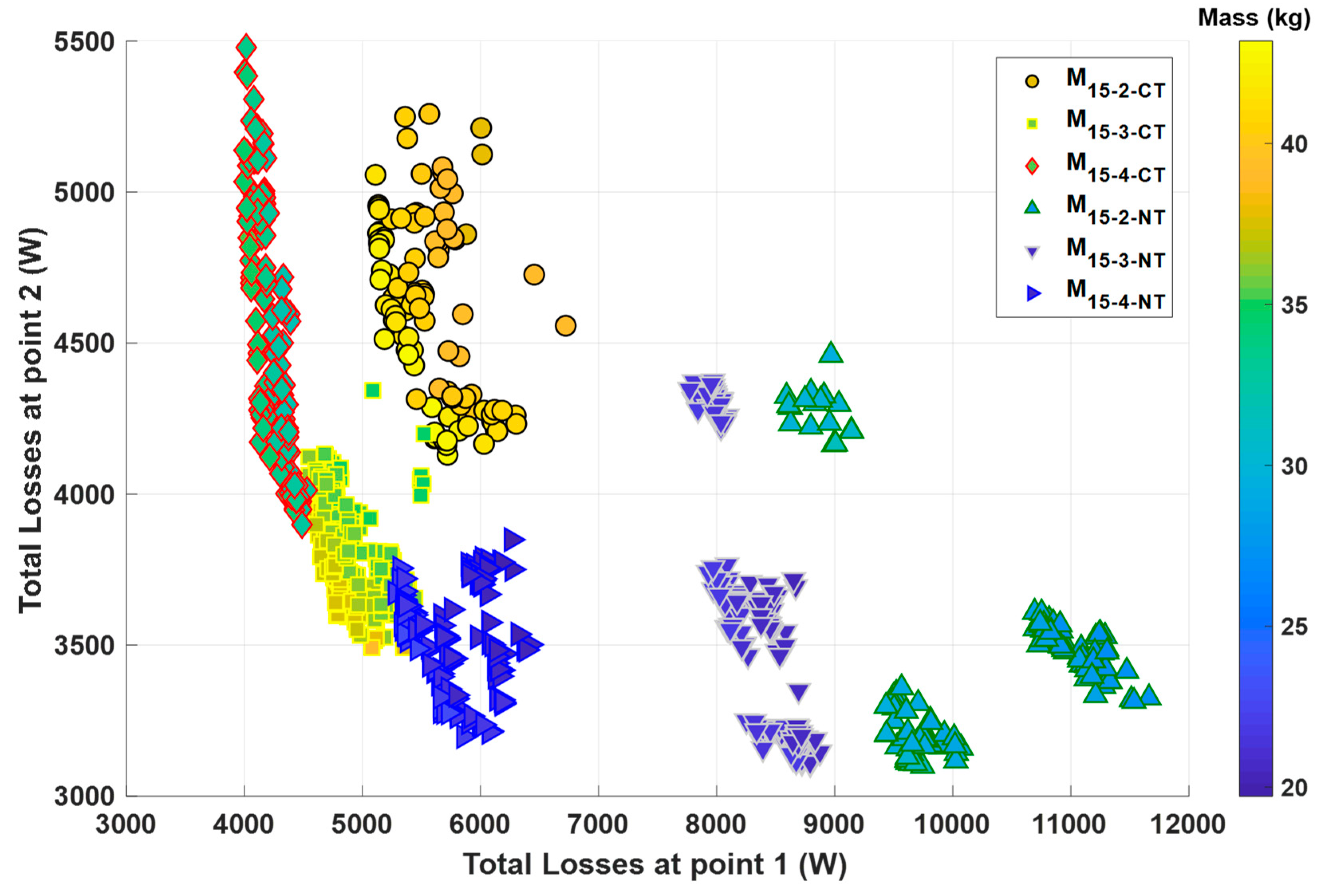
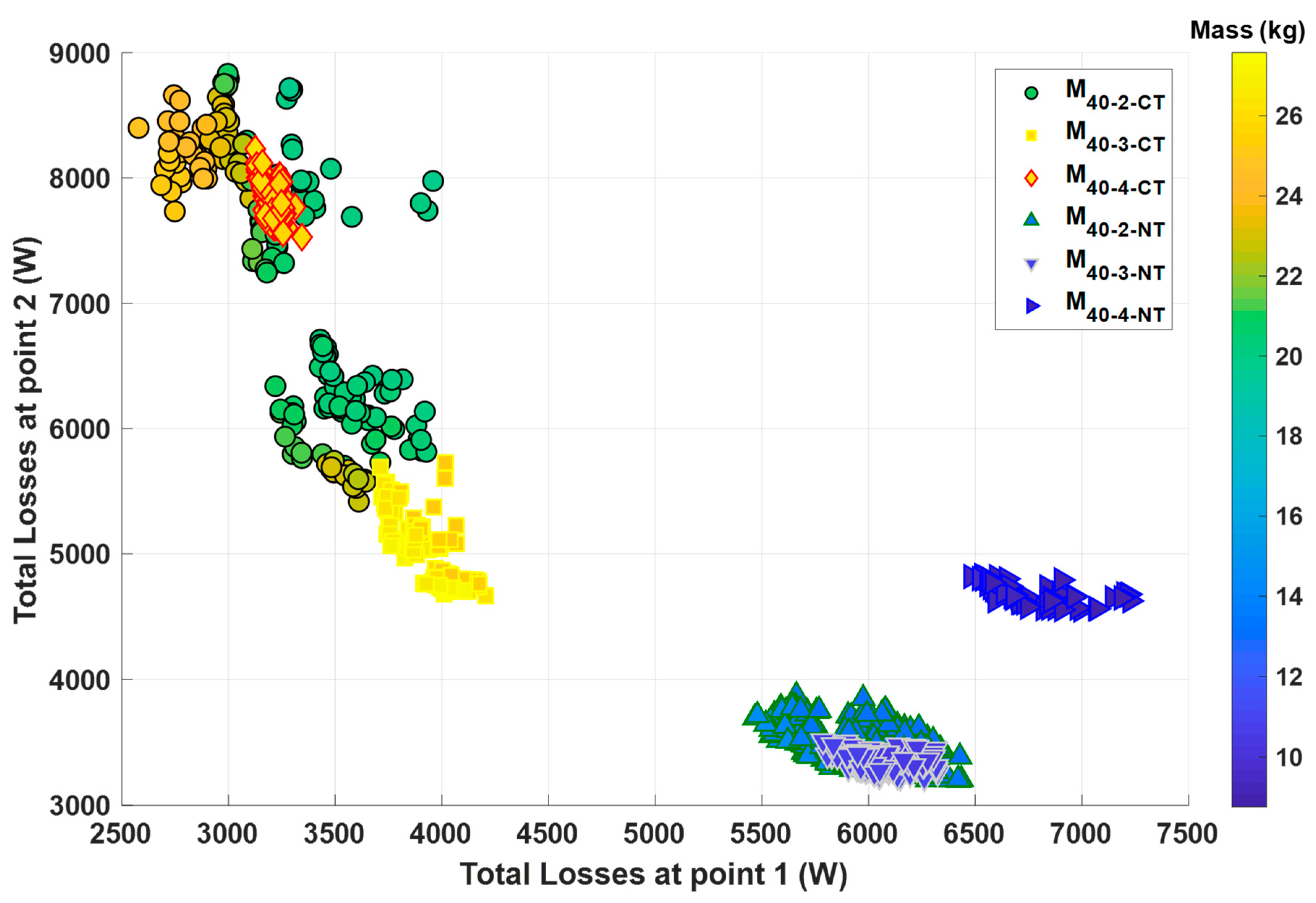
Figure 8 represents the pareto front of machines using both classic and new technologies operating at Ω m a x = 15,000   rpm with p = 2, 3, and 4.
For classic technologies, machines with p = 4 have the lowest losses at point 1 (4–4.5 kW), high losses at point 2 (4–5.5 kW), and the lowest mass (32–35) kg. Machines with p = 3 have medium losses at point 1 (4.5–5.5 kW), the lowest losses at point 2 (3.5–4.2 kW), and medium mass (35–39 kg). Machines with p = 2 have the highest losses at point 1 (5.1–6.7 kW), high losses at point 2 (4.1–5.3 kW), and high mass (38–43 kg). Therefore, electric machines using classic technologies with p = 4 are the best candidates since they have the lowest mass and the best efficiency.
For new technologies, machines with p = 4 have the lowest losses at point 1 (5.2–6.4 kW), low losses at point 2 varying from 3.2 to 3.8 kW, and a low mass varying from 20 to 23 kg. Machines with p = 3 have medium losses at point 1 (7.7–8.8 kW), losses at point 2 mostly varying from 3.1 to 4.4 kW, and low mass (20.5–21.8 kg). Machines with p = 2 have the highest losses at point 1 (8.5–11.6 kW), losses at point 2 varying from 3 to 4.5 kW, and high mass (27–31 kg). Hence, electric machines using new technologies with p = 3 and p = 4 have the same range of mass, but the latter have better efficiency.
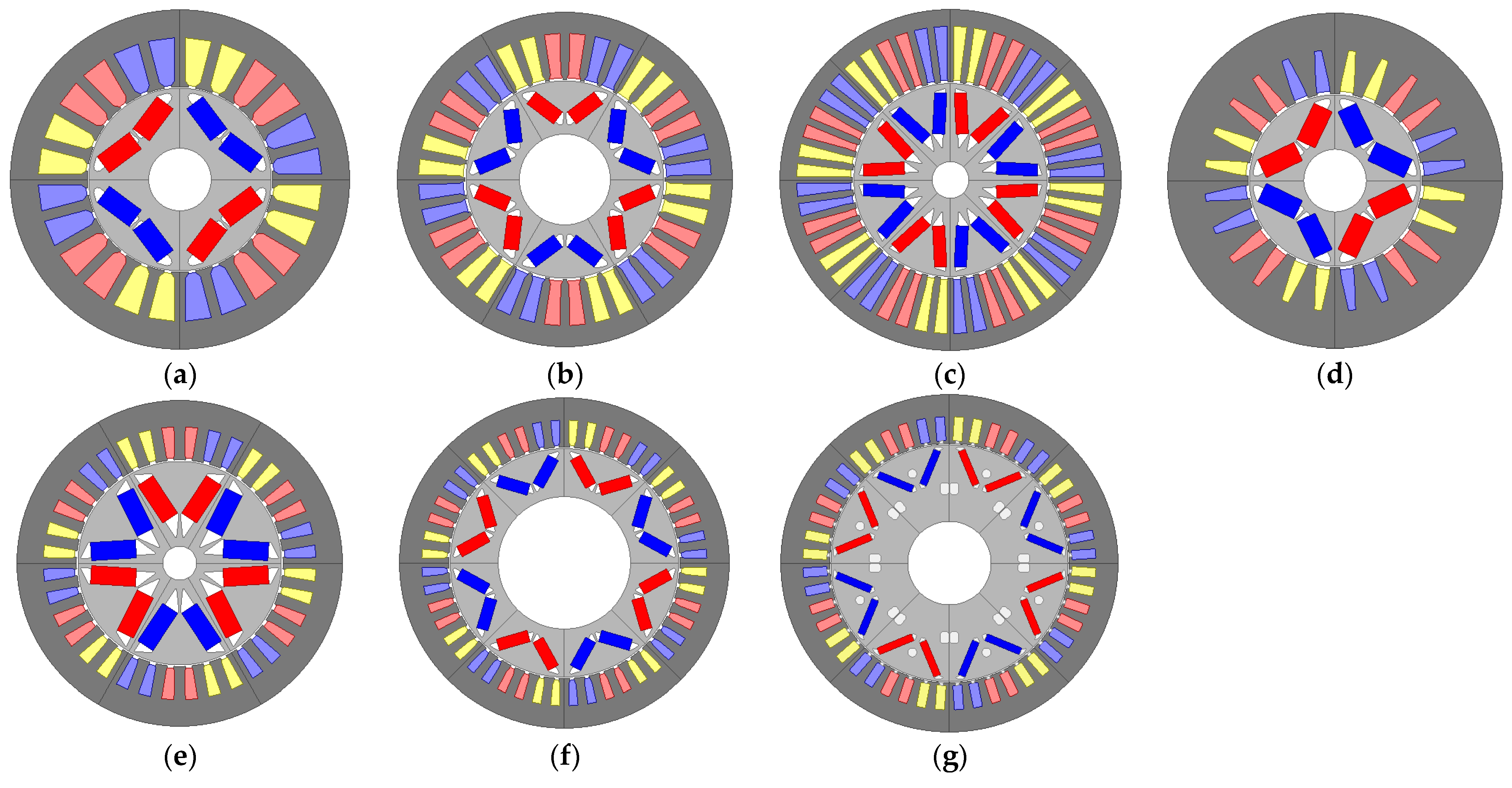
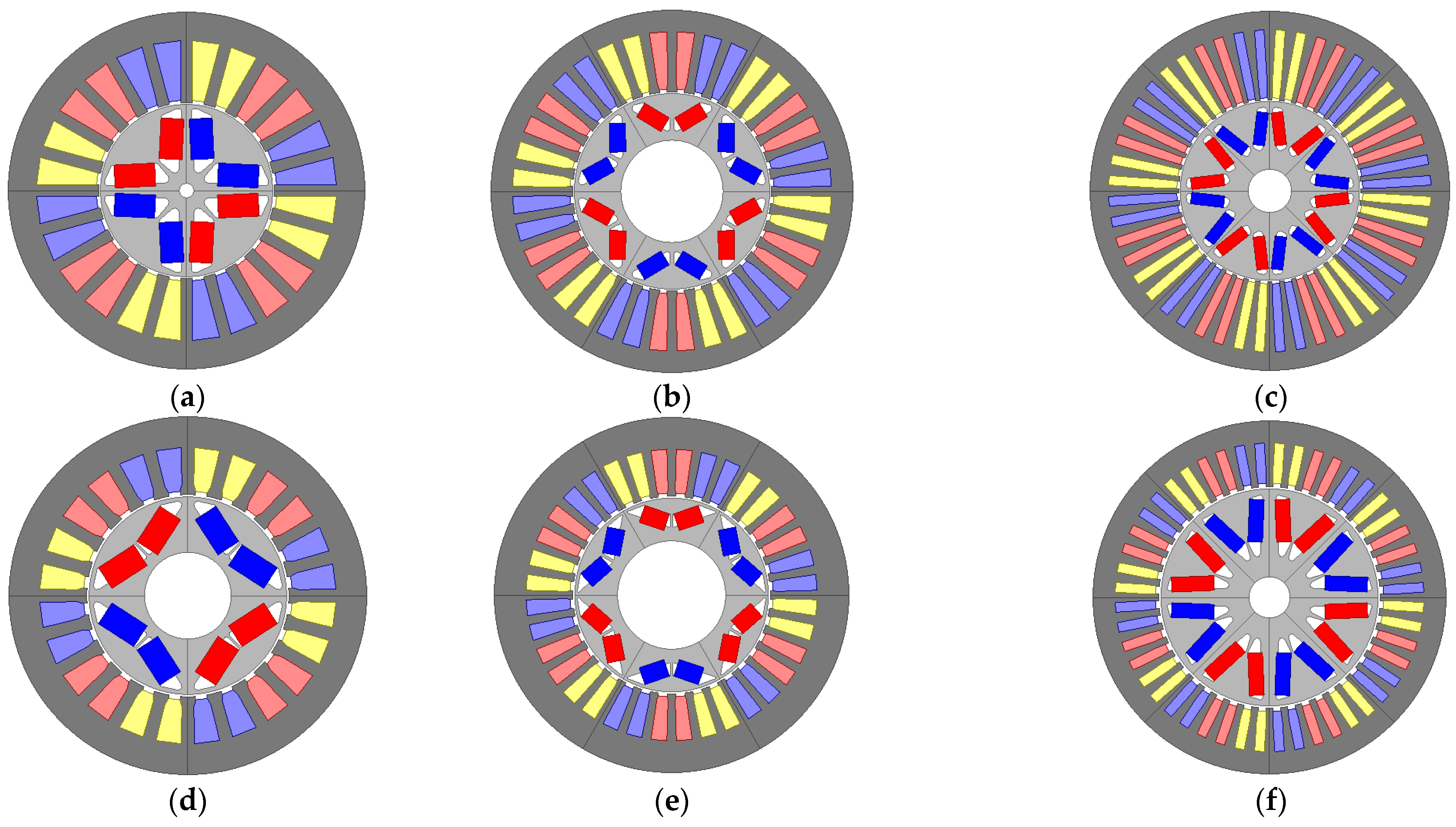
In the following, we select the machine with the highest power density for each pole pair and technology type, which will be compared to the electric machine used in Peugeot e208. These selected machines are represented in Figure 9, and their characteristics are listed in Table 5.
For CT-based machines, at point 1, iron losses increase with the number of pole pairs due to frequency. At point 2, the machine with p = 2 has high iron losses compared to machines with p = 4 and p = 3. The machine with p = 2 has a higher magnet flux because of the high number of turns, thus inducing more iron losses. Due to frequency, AC losses at points 1 and 2 increase with the number of pole pairs. Contrarily, joule losses at points 1 and 2 decrease by increasing the number of pole pairs. Indeed, decreasing the number of pole pairs leads to increasing the number of turns due to the voltage constraint. Consequently, the resistance, expressed as a function of the square of the number of turns, increases by decreasing the number of pairs of poles, leading to higher joules losses. Moreover, all machines have a high current density (14 Arms/mm²). It cannot be further increased due to the current reaching its maximal value defined in specifications (445 Arms), mainly due to the low number of turns. The current at point 2 increases with the number of pole pairs because of the need to flux weaken the machine at high frequency. It is important to note that joule and iron losses are dominant at points 1 and 2, respectively.
For NT-based machines, the number of pole pairs is also decreased by increasing the number of turns due to voltage constraints. Given the low number of turns of the machine with p = 4, its current density at point 1 is limited to 27.2 Arms/mm² because of the current reaching its maximal value defined in specifications, unlike machines with p = 2 and p = 3, whose current density at point 1 exceeds 31 Arms/mm² thanks to a higher number of turns. NT-based machines have slots with a small surface, which, given the same number of turns, leads to higher resistance per phase than CT-based machines. The current at point 1 is of the same magnitude as CT-based machines; this explains why joule losses are higher for NT-based machines. Similarly, joule losses increase by decreasing the number of pole pairs for the same reasons mentioned previously. Iron losses increase with the number of pole pairs due to frequency. Iron losses are lower for NT-based machines thanks to thinner laminations. To satisfy the required high filling factor, the optimization selects a smaller diameter and a greater number of strands in parallel compared to CT-based machines. This explains the low AC losses. The use of new technologies reduces efficiency at low speed (point 1) and increases efficiency at high speed (point 2).
The use of new technologies allows for having more compact machines, which leads to high power density and low amounts of magnets and copper for the three studied pole pairs values. We notice that the power density increases with the number of pole pairs for CT-based machines. The machine with p = 4 has the highest power density (18.9kW/L) with the best efficiency at point 1 (95.9%), good efficiency at point 2 (96%), a high amount of magnets (31 g/kW), and the lowest amount of copper (68.6g/kW). With a nearly similar amount of magnets, the machine with p = 2 has the lowest power density (15.5 kW/L), a low efficiency at points 1 (94.4%) and 2 (95.2%), and the highest amount of copper (92%). Therefore, the machine with p = 2 is not optimal. The machine with p = 3 has the lowest amount of magnets (26.8 g/kW), good efficiency at points 1 (95.5%), and 2 (95.9%) but a low power density (16.3 kW/L). Finally, the CT-based machine with p = 4 can be considered the best candidate.
For NT-based machines, results show that the machine with p = 3 has the highest power density (32.7 kW/L), the highest amount of magnets (24.6 g/kW), and a medium efficiency at points 1 (92.2%) and 2 (96.6%). The machine with p = 4 uses the lowest amount of magnets (16.8 g/kW) with the best efficiency at point 1 (94.3%) and point 2 (96.8%) and medium power density (28.8 kW/L). The machine with p = 2 has the lowest power density (24.4kW/L), low efficiency at point 1 (89.9%), and the highest amount of copper (42.2%), which makes it not optimal. Thus, the NT-based machine with p = 4 can be considered the best compromise regarding the amount of magnets.
Peugeot e208′s machine has a maximum current density of 16 Arms/mm² and uses 0.35 mm thickness laminations and a high fill factor thanks to hairpin windings. Therefore, it can be considered a CT-based machine. Based on obtained results, among all the CT-based machines, the machine with p = 4 has the highest power density (18.9 kW/L), while for the NT machines, using three pole pairs leads to the best power density (32.7 kW/L). These results can explain Peugeot’s choice of four pole pairs for its electric vehicle e208′s CT-based V-shaped IPMSM operating at Ω m a x = 14,000   rpm . However, the latter has a low power density (18 kW/L) compared to the optimized machines in this work. On the one hand, this can be explained by a slightly lower maximum rotational speed and, on the other hand, by the fact that Peugeot e208′s machine has been optimized by considering the machine’s price. The price of magnets being the highest explains the choice of the low amount of magnets used in the Peugeot e208 (18 g/kW) compared to optimized CT-based machines, as shown in Table 5. To guarantee the required performances, this reduction in the amount of magnets is made at the expense of other cheaper machine materials (iron and/or copper), which explains the low power density of the e208′s machine. Only NT-based machines allow a lower amount of magnets.

5.2. Maximum Rotation Speed Ω m a x = 20,000 rpm

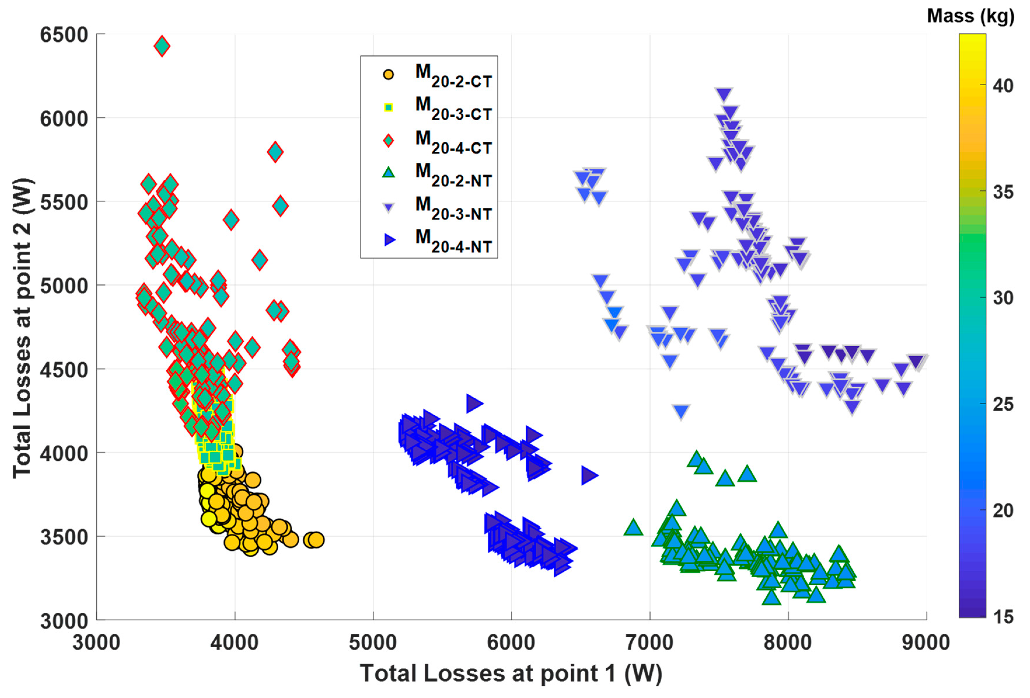
Figure 10 represents the Pareto front of machines using both classic and new technologies operating at Ω m a x = 20,000   rpm with p = 2, 3, and 4.
For classic technologies, machines with p = 4 have the lowest losses at point 1 (3.3–4.4 kW), the highest losses at point 2 (4.1–6.5 kW), and low mass (28.5–32.5 kg). Machines with p = 3 have medium losses at point 1 (3.7–4 kW), medium losses at point 2 (3.9–4.5 kW), and low mass (28.5–30.5 kg). Machines with p = 2 have the highest losses at point 1 (3.8–4.6 kW), the lowest losses at point 2 (3.4–4.3 kW), and high mass (38–42.3 kg). Machines with p = 3 can be considered the best candidates regarding their good efficiency and low mass.
For new technologies, machines with p = 4 have the lowest losses at point 1 (5.2–6.6 kW), low losses at point 2 (3.3–4.3 kW), and low mass (15–16.2 kg). Machines with p = 3 have high point 1 losses (6.5–9 kW), high point 2 losses (4.2–6.1 kW), and low mass (15–21 kg). Machines with p = 2 have high losses at point 1 (6.9–8.4 kW), low losses at point 2 (3.1–3.9 kW), and high mass (23.4–24.9 kg). Machines with p = 3 and p = 4 have low mass with the same order of magnitude, but the latter has higher efficiency at points 1 and 2.
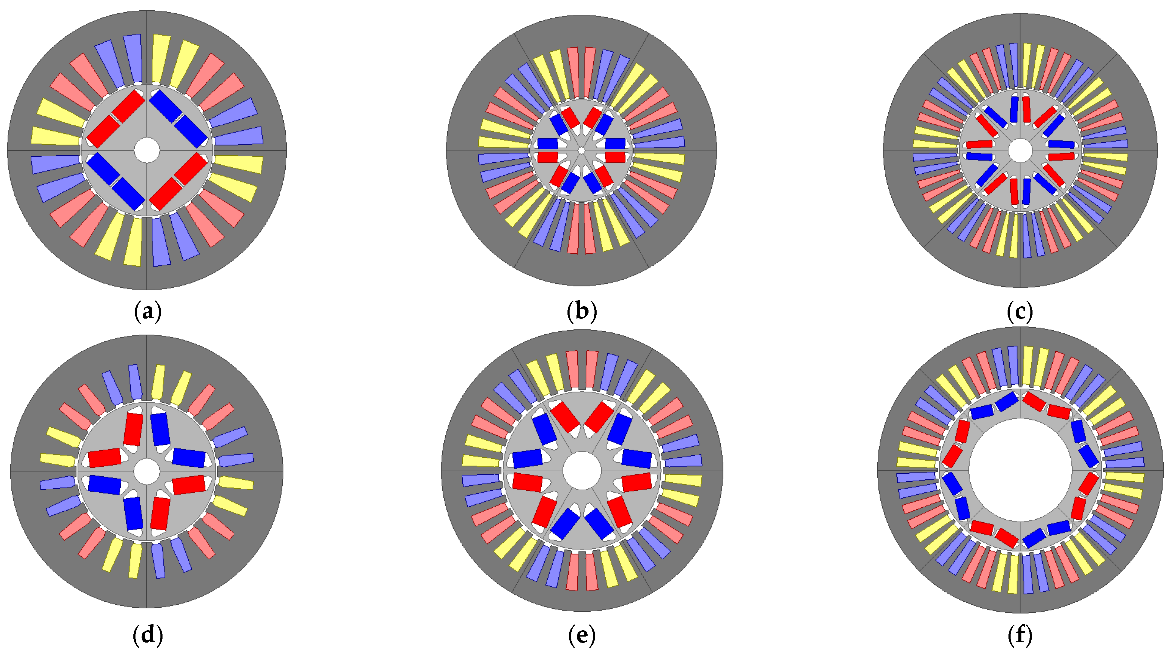
In the following, we select the machine with the best power density for each pole pair value and technology type, which will be compared to the electric machine used in Tesla Model 3. These selected machines are represented in Figure 11, and their characteristics are listed in Table 6.
For CT-based machines, we notice that joule losses increase as the number of pole pairs decreases due to the increase of resistance for the reasons mentioned previously. Iron losses increase with the number of pole pairs because of the frequency. AC losses are of the same magnitude for machines with p = 2 and p = 3. The machine with p = 4 has higher AC losses due to higher frequency. Moreover, the dominant losses at points 1 and 2 are joule and iron losses, respectively. The number of turns decreases as the number of pole pairs increases due to voltage constraints. The machine with p = 2 has four turns, while machines with p = 3 and p = 4 have two turns. The resistance per phase, expressed as the square of the number of turns, is, therefore, higher for the machine with p = 2. With the same number of turns, machines with p = 3 and p = 4 have similar resistance per phase. To reach the torque for the machine with p = 3, the current density is increased to its maximum value (15 Arms/mm²) due to a low number of turns, which leads to a current nearly reaching its maximal value defined in specifications (442 Arms).
For NT-based machines, we observe that joule losses are very high compared to CT-based machines. Indeed, high current density allows reaching the same ampere-turns with a small copper surface area. Therefore, the resistance per phase is higher, which leads to higher joules losses. Contrarily, iron losses are low compared to CT-based machines, thanks to thinner laminations. For example, for the machine with p = 4, iron losses are equal to 600 W (2.5 kW) at point 1 (point 2) using CT, while they are equal to 300 W (1.5 kW) at point 1 (point 2) using NT. Machines with p = 2, p = 3, and p = 4 have 4, 3, and 2 turns, respectively. This choice is made based on voltage constraints. Machines based on new technologies are more compact, allowing the machine with p = 3 to have slightly more turns than the same machine with CT. The current density for the machine with p = 3 reaches its maximal value defined in specifications (33 Arms/mm²). In contrast, the machine with p = 4 is limited to 25.9 A/mm² due to the current limitation caused by the low number of turns. Moreover, joule losses are dominant at point 1. Given the high resistance value, joule losses are also dominant at point 2 except for the machine with p = 4, for which iron losses are significant due to frequency.
Tesla Model 3′s machine uses 0,25 mm thickness laminations, a current density of 33.7 Arms/mm², and a classic fill factor of 45%. Therefore, it can be considered an NT-based machine. Using CT, the machine with p = 3 has the highest power density (21 kW/L), good efficiency at points 1 (96.3%) and 2 (96%), and the lowest amount of copper (53.3 g/kW) but the highest amount of magnets (25.4 g/kW). The machine with p = 4 has a power density reaching 19.8 kW/L, good efficiency at points 1 (96.5%) and 2 (95.2%), and a low amount of magnets (20.1 g/kW) and copper (60.7 g/kW). With a low power density reaching 15.7 kW/L and a very high amount of copper (86.9 g/kW), the machine with p = 2 is the least favorable despite its high efficiency. The CT-based machine with p = 4 can be considered the best compromise regarding the low amount of magnets and a power density nearly similar to that of the machine with p = 3.
NT allows for increasing the power density and reducing the amount of copper and magnets. The machine with p = 3 has the best power density reaching 42.14 kW/L and the lowest amount of copper (27.7 g/kW) but uses the highest amount of magnets (21.5g/kW) and has low efficiency at points 1 (92.6%) and 2 (95.2%). The machine with p = 4 has a lower power density (36.47 kW/L), the lowest amount of magnets (12.3 g/kW), and better efficiency at points 1 (94.3%) and 2 (96.3%). With a low power density of 28.94 kW/L and a high amount of copper (39 g/kW), the machine with p = 2 is the least favorable among NT-based machines.
The machine with p = 3 is the best candidate in terms of power density for both technologies. This can explain Tesla’s choice of three pole pairs for its electric vehicle Model 3′s NT-based V-shaped IPMSM operating at Ω m a x = 18,000   rpm . Although the Tesla Model 3′s machine has a high power density of 37.5kW/L, it is lower than the optimized NT-based machine with p = 3. This difference can be explained, on the one hand, by a lower maximum rotational speed used by Tesla and, on the other hand, by the fact that the fill factor is higher for the optimized NT-based machines.
The NT-based machine with p = 3 uses 21.52 g/kW of magnets, higher than the Tesla Model 3′s machine with 8.91 g/kW of magnets. This can be explained by the fact that the latter has been optimized by considering an additional dimension, which is the machine’s price. As mentioned previously, the reduction in the amount of magnets, the most expensive material of the machine, is done to the detriment of the amount of iron and/or copper. This necessarily results in a machine with high mass, which explains the low power density of Model 3′s machine compared to the optimal NT-based machine with p = 3. Tesla opted for a low DC voltage (350 V) with parallel windings to respect the voltage constraint. Therefore, it requires a higher maximum current (850 Arms/mm²) to reach the maximal torque. In addition, Tesla opted for three slots per pole and per phase and a 0.9 mm air gap length, which allows for reducing harmonics losses.
With a power density of 42 kW/L, the NT-based machine with p = 3 is the candidate that nearly reaches the objective 50 kW/L power density set by the US Drive 2025 project. It is possible to further improve the power density by increasing the DC voltage, thus increasing the number of turns and increasing magnet flux. Increasing the maximum current density can also allow for reaching the 50 kW/L objective, but this will require the design of newer cooling techniques than those currently used, such as the cooling of end windings with oil sprays used in Tesla Model 3′s machine.

5.3. Maximum Rotation Speed Ω m a x = 30,000 rpm

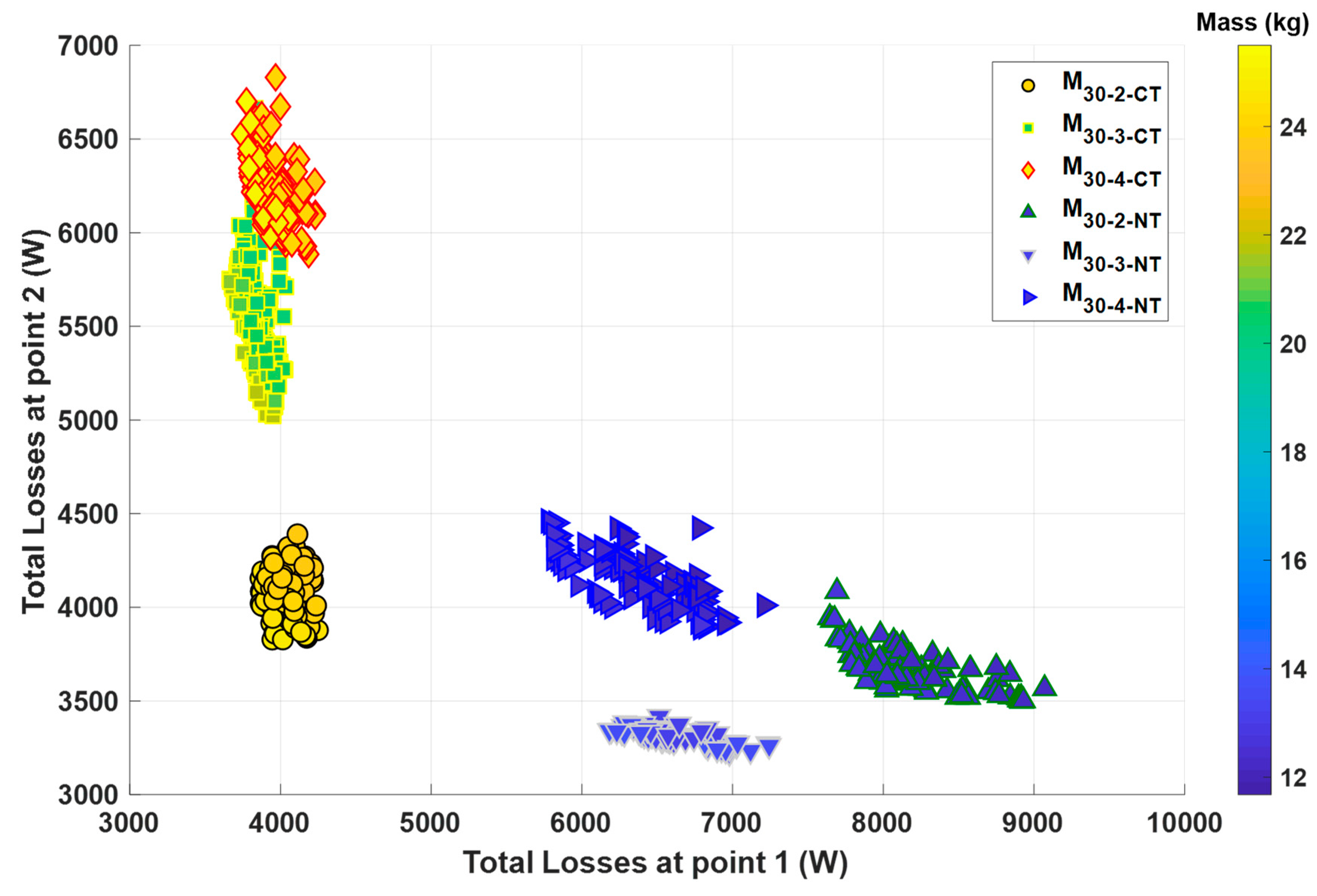
Figure 12 represents the pareto front of machines using both classical and new technologies operating at Ω m a x = 30,000   rpm with p = 2, 3, and 4.
For classic technologies, machines with p = 4 have medium losses at point 1 (3.7–4.2 kW), the highest losses at point 2 (5.9–6.8 kW), and high mass (23.5–25.5 kg). Machines with p = 3 have low losses at point 1 (3.6–4 kW), medium losses at point 2 (5–6.6 kW), and low mass (20–22 kg). Machines with p = 2 have high losses at point 1 (3.8–4.2 kW), the lowest losses at point 2 (3.8–4.4 kW), and medium mass (23.5–24.8 kg). Machines with p = 3 can be considered the best candidate regarding their mass and efficiency.
For new technologies, machines with p = 4 have low losses at point 1 (5.8–7.2 kW), high losses at point 2 (3.9–4.5 kW), and low mass (11.8–12.7 kg). Machines with p = 3 have low losses at point 1 (6.2–7.3 kW), low losses at point 2 (3.2–3.4 kW), and high mass (13–13.7 kg). Machines with p = 2 have high losses at point 1 (7.6–9.1 kW), medium losses at point 2 (3.5–4.1 kW), and medium mass (12.1–12.9 kg). Machines with p = 4 are the best candidate regarding their mass and efficiency.
In the following, we select the machine with the best power density for each pole pairs and for each technology type, which will be compared to the machine designed by AVL [23] operating at 30,000   rpm 
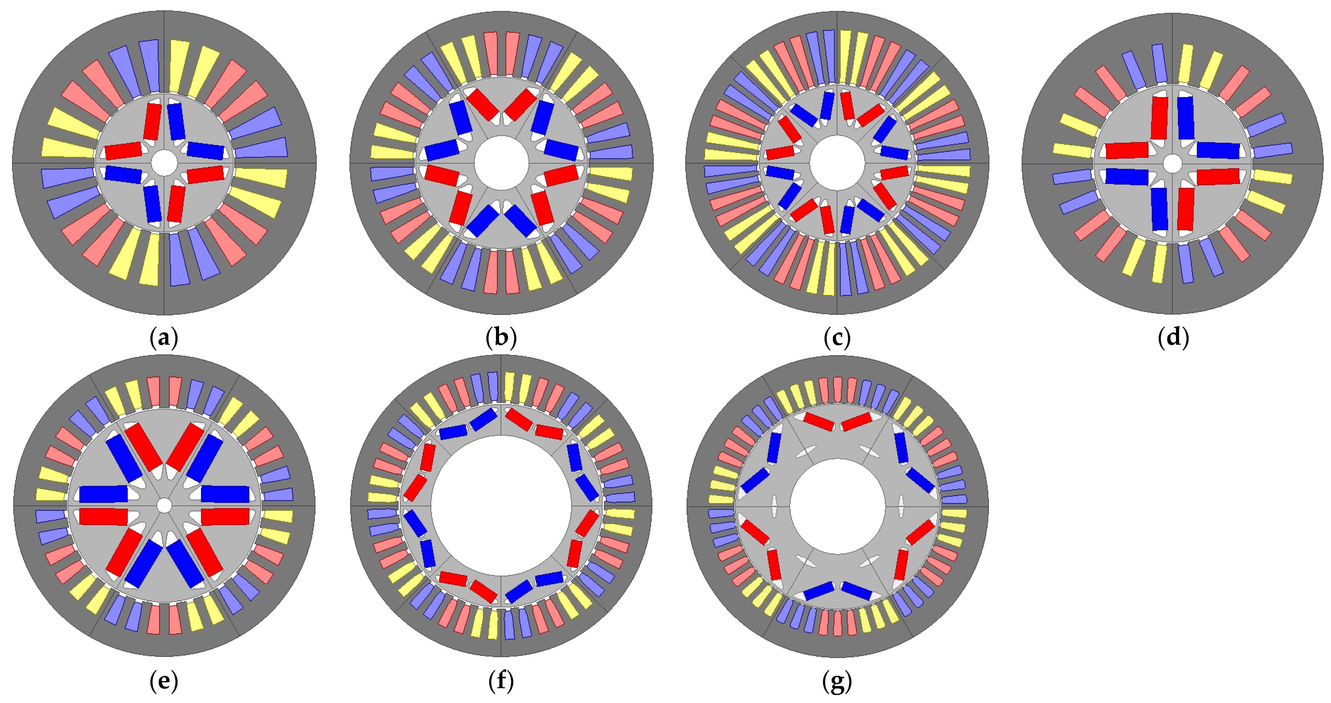
. Optimized machines are represented in Figure 13 and their characteristics are listed in Table 7.
For CT-based machines, we notice that joule losses decrease by increasing the number of pole pairs, as observed for previous maximum rotational speed values. Due to frequency, iron and AC losses increase with the number of pole pairs. Joule and iron losses are dominant at points 1 and 2, respectively. The machine with p = 2 has three turns, while machines with p = 3 and p = 4 have two turns due to voltage constraints. Consequently, the resistance per phase is higher for the machine with p = 2, which explains its high joule losses. Joule losses are very predominant at point 1; this explains why the machine with p = 2 has high losses at point 1. Iron losses being the majority at point 2, the machine with p = 4 has the highest losses at point 2.
For NT, the machines with p = 2, p = 3, and p = 4 have 4, 3, and 2 turns, respectively, higher than CT-based machines because of more compact machines. Thanks to a high current density, a small amount of copper surface area is required to reach the same ampere-turns, which, added to an increased number of turns, leads to high resistance per phase. The current being of the same order of magnitude between machines of both technologies, joules losses are therefore higher for NT-based machines. Hence, losses at point 1, composed mainly of joules losses, are higher than CT-based machines. However, losses at point 2 are lower thanks to thinner laminations, which remarkably reduce iron losses. The high number of turns can also help minimize iron losses [40]. Indeed, although magnet flux increases as a function of the number of turns, the inductance increases as a function of the square of the number of turns, therefore, allowing the reduction of flux generated by the rotation of rotor/magnets. The machine with p = 3 has a current density at point 1 of 26.2 Arms/mm², lower than other machines because of the current limitation.
The 0.2 mm thickness laminations chosen by AVL drastically reduce iron losses. Little information is provided regarding the current density used by AVL. However, since the cooling system consists of injecting oil into the closed slots of the stator, the current density is necessarily higher than the usual value of 15 Arms/mm². Therefore, AVL’s machine can be considered an NT-based machine.
For CT, the machine with p = 3 has the highest power density (27.8 kW/L), the lowest amount of magnets (12.9 g/kW) and copper (48.5 g/kW), and the highest efficiency at point 1 (96.4%). The machine with p = 4 has the lowest power density (24.8 kW/L), high efficiency, and a medium amount of magnets (15.6 g/kW) and copper (57.1 g/kW). The machine with p = 2 has a low power density (25.2 kW/L), a high amount of magnets (18.9 g/kW) and copper (60.1 g/kW), and good efficiency. Thus, the CT-based machine with p = 3 is the best candidate.
For NT, the machine with p = 4 has the highest power density (57.7 kW/L), good efficiency, the lowest amount of copper (22.3 g/kW), and the highest amount of magnets (12.5g/kW). The machine with p = 3 has the lowest power density (48.1 kW/L), unlike the CT-based machine with p = 3. Its main advantage is the high efficiency and the low amount of magnets (7.9 g/kW). The machine with p = 2 has a medium power density (53.4 kW/L), a medium amount of magnets (10.6 g/kW) and copper (30.1 g/kW), and a low efficiency at point 1. Thus, for NT-based machines, the machine with p = 4 represents a reasonable compromise, followed by the machine with p = 2. The advantages of the machine with p = 3 are the low amount of magnets (7.9 g/kW) and the excellent efficiency. This can explain AVL’s choice of tree pole pairs for its designed NT-based V-shaped IPMSM. AVL’s machine and the optimized NT-based machine with p = 3 have power density equal to 45.5 kW/L and 48.12 kW/L, respectively. The high fill factor used for the optimized machine in this work can explain this slight difference. Further, AVL’s machine has closed slots, which allows for reducing harmonics losses and, therefore, the use of a 0.7 mm air gap length lower than Tesla Model 3′s machine. The information concerning the winding’s configuration has not been provided by AVL; however, given the maximum current value of 525 A and the high DC voltage of 800 V, the winding is probably in series, similar to the optimized machines.

5.4. Maximum Rotation Speed Ω m a x = 40,000 rpm

Figure 14 represents the Pareto front of machines using both classical and new technologies operating at Ω m a x = 40,000   rpm with p = 2, 3, and 4.
For classic technologies, machines with p = 4 have medium losses at point 1 (3.1–3.3 kW), high losses at point 2 (7.5–8.2 kW), and high mass (25.5–26.4 kg). Machines with p = 3 have high losses at point 1 (3.7–4.2 kW), low losses at point 2 (4.6–5.7 kW), and high mass (25–27.5 kg). Machines with p = 2 have low losses at point 1 (2.6–4 kW), medium and high losses at point 2 (5.4–8.8 kW), and low mass (19.8–25 kg). Its losses at points 1 and 2 vary over a wide range of values. They can be separated into two groups: a first group where the losses at point 1 are high and the losses at point 2 are low and a second group where the losses at point 1 are low and the losses at point 2 are high. Machines with p = 2 are the best candidates in terms of mass.
For new technologies, machines with p = 4 have high losses at point 1 (6.45–7.25 kW), high losses at point 2 (4.5–4.8 kW), and low mass (8.8–9.4 kg). Machines with p = 3 have low losses at point 1 (5.8–6.35 kW), low losses at point 2 (3.2–3.5 kW), and medium mass (10.3–11.1 kg). Machines with p = 2 have low losses at point 1 (5.4–6.4 kW), low losses at point 2 (3.2–3.9 kW), and high mass (13–14.4 kg). Machines with p = 4 have the lowest mass, but the machines with p = 3 can be considered the best compromise in terms of mass and efficiency.
In the following, we select the machine with the best power density for each pole pairs and each technology type. These selected machines are represented in Figure 15, and their characteristics are listed in Table 8.
For classic technologies, the machine with p = 2 has the highest power density (30.3 kW/L), unlike previous values of maximum rotational speed for CT-based machines, with excellent efficiency at point 1 (96.9%) and medium efficiency at point 2 (92.6%). Its main disadvantages compared to other pole pairs are the highest amount of copper (42.6 g/kW) and magnets (13.4 g/kW). The machine with p = 4 has low power density (25.5 kW/L), good efficiency at point 1 (96.8%), low efficiency at point 2 (93%), the lowest amount of copper (32.4 g/kW), and high amount of magnets (12.7 g/kW). To respect the voltage constraint, the machine with p = 4 has one turn, resulting in a low magnet flux. The current density is limited to 14.2 Arms/mm² because of the current reaching its maximal value defined in specifications. The low number of turns leads to a low magnet flux and ampere-turns; hence, the optimization chooses a higher active length to achieve the required torque. The maximum active length initially defined as 200 mm has been increased to 210 mm for machines with p = 4 to reach the required torque. This results in a larger machine and, therefore, lower power density. With a single turn, the resistance per phase is low, which results in lower joule losses (2 kW at point 1). The latter is dominant at low speed; therefore, total losses at point 1 of the machines with p = 4 are low. Moreover, a small number of turns induces more iron losses [40] at point 1 (1 kW) and point 2 (4.6 kW). The latter being dominant at high speed explains the high total losses at point 2 for the machine with p = 4. The machine with p = 3 has low power density (25kW/L), good efficiency at point 1 (96.3%) and point 2 (95.3%), a medium amount of magnets (11.6 g/kW), and a high amount of copper (43.3 g/kW). It has two turns, which allows more ampere-turns. Therefore, the optimization slightly increases the current density to 14.4 Arms/mm2 and increases the slot’s surface thanks to the high outer radii of the stator. Furthermore, a higher number of turns means a higher resistance per phase and, therefore, higher joule losses (2.8 kW at point 1). The latter being dominant at low speed, total losses at point 1 of the machine with p = 3 are therefore high.
In order to design a machine, it is usual to choose a high number of pole pairs to reduce the volume of the machine. However, this conventional technique cannot be applied at high speed due to the limitations of the number of turns related to voltage constraints. Indeed, the results above show that the CT-based machine with p = 2 has the highest power density, contrary to the previous values of maximum rotational speed for CT-based machines.
For NT-based machines, the machine with p = 4 has the highest power density (68.2 kW/L) with the lowest amount of magnets (6 g/kW). It has the highest joule losses at point 1 (6.4 kW), unlike the previous values of maximum rotational speed for NT-based machines. Its iron losses (1.8 kW at point 2) are also high, which explains the lowest efficiency at point 1 (93.6%) and point 2 (95.7%). It has the lowest mass, unlike the CT-based machine with p = 4. This can be explained by the absence of the previously mentioned limitations thanks to a more compact machine and hence, a higher number of turns (two compared to one for CT-based machine), which no longer requires a high active length to reach the required torque. Once the limitations are lifted, thanks to the use of new technologies, increasing the number of pairs of poles leads to less voluminous machines. The machine with p = 2 is not optimal due to a low power density (52 kW/L) and high amount of magnets (8.9g/kW) despite its high efficiency at point 1 (94.2%) and point 2 (96.6%). The machine with p = 3 has a medium power density (63.9 kW/L) and high efficiency at points 1 (94.2%) and 2 (96.8%). However, its major drawback is the high amount of magnets (9.4 g/kW). Due to the current limitation, it has a high active length, allowing reaching the required torque. For NT, both machines with p = 3 and p = 4 can be considered a good compromise between the efficiency and the magnet’s amount. Although the amount of magnets is higher for the former, it is possible to reduce their cost. To do this, we can apply the solution proposed by AVL consisting of using magnets without rare earth, namely dysprosium (Dy) and terbium (Tb). Therefore, it is essential to perform a fine thermal analysis of the machine and to design new cooling techniques to avoid the demagnetization of the magnets.

5.5. Comparisons and Conclusions

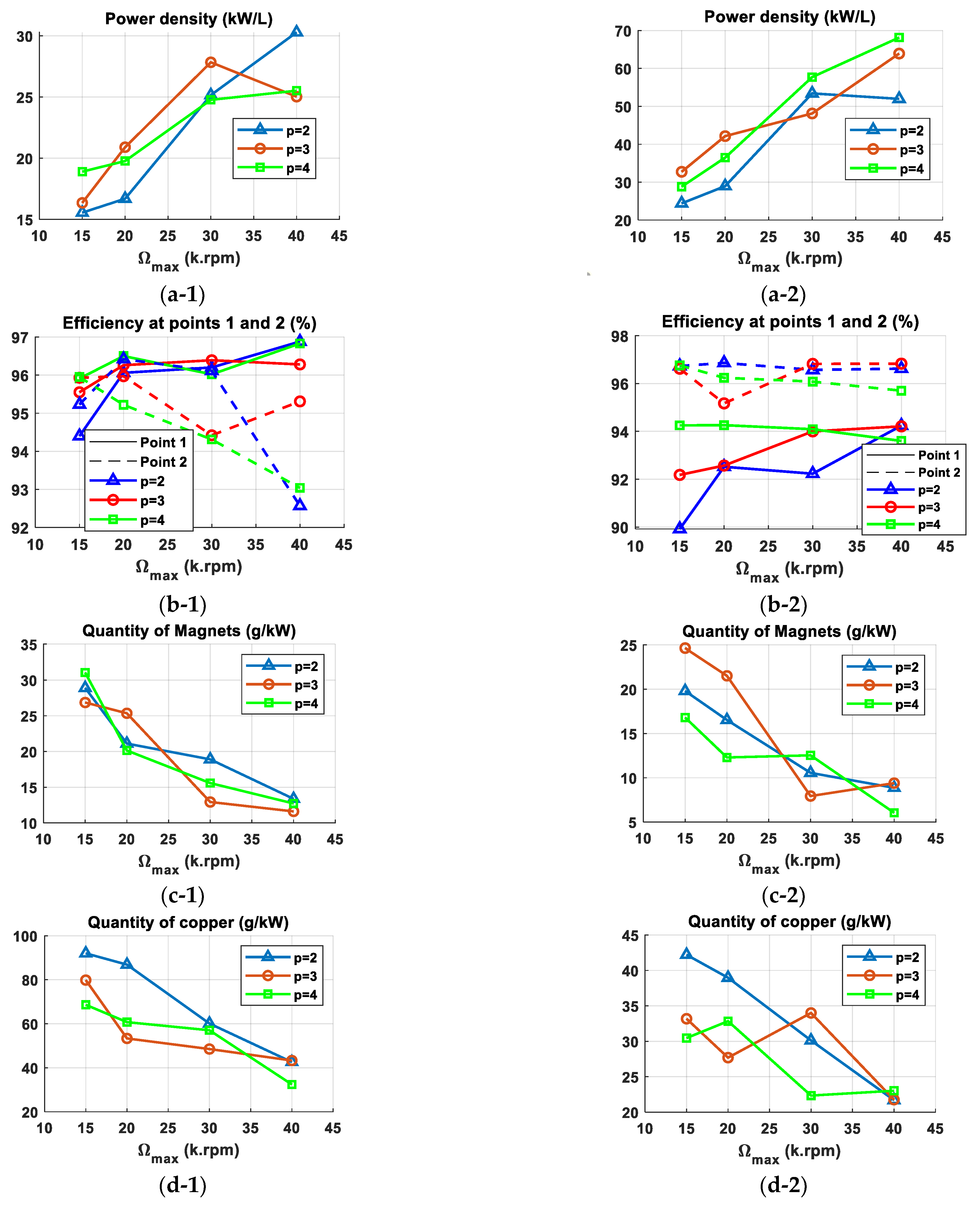
Figure 16 represents the performances and characteristics of the optimal machines previously selected for each pole pairs, maximum rotational speed, and technology type. These characteristics are the power density, the efficiency at points 1 and 2, and the amount of magnets and copper. We notice that the power densities reached at Ω m a x = 40,000   rpm using classic technologies are of the same order of magnitude as the power densities reached at Ω m a x = 15,000   rpm using new technologies. Thus, to achieve high power density while avoiding problems related to bearings limitations and vibrations at high speed, it is preferable to use new technologies with a maximum rotational speed Ω m a x up to 20,000   rpm . Further, the machine M 3 20 N T allows 57% volume reduction compared to the machine currently used in the Peugeot e208. This achievement matches the Europe Union’s ambitions of reducing machines' raw materials [41]. However, the density of losses in these compact machines increases considerably due to the high fill factor and current density. Therefore, future work needs to be conducted on innovative cooling techniques to evacuate generated losses.
New technologies allow more compact machines, reducing the amount of copper and magnets. The efficiency at point 1 is often reduced with the use of NT because of higher joule losses due to a higher resistance per phase. Indeed, a small copper’s surface is needed thanks to high current density. However, the efficiency at point 2 is improved with the use of NT thanks to a significant reduction of iron losses due to the use of thinner laminations. The high number of turns of some NT-based machines also contributes to reducing iron losses.
For CT-based machines, the number of pole pairs allowing the highest power density decreases when increasing the maximum rotational speed, as shown in Figure 16. At Ω m a x = 15,000   rpm , the machine with p = 4 is the best candidate in terms of power density (18.9 kW/L). At Ω m a x = 20,000   rpm , the machine with p = 3 is the best candidate in terms of power density (20.9 kW/L), closely followed by the machine with p = 4 (19.77 kW/L). The latter can be chosen given its low amount of magnets (20.14 g/kW) compared to the machine with p = 3 (25.35 g/kW). At Ω m a x = 30,000   rpm , the machine with p = 3 is by far the best candidate thanks to its high power density (27.84 kW/L), low amount of magnets (12.93g/kW), low amount of copper (48.52 g/kW), and high efficiency at point 1 (96.39%) and point 2 (94.42%). At Ω m a x = 40,000   rpm , the machine with p = 2 has the best power density, reaching 30.28 kW/L; an amount of magnets, 13.37g/kW, slightly higher than other machines; and a low efficiency at point 2 of 92.57%. As mentioned previously, the number of pole pairs is usually considered when choosing a machine with low volume. However, this property is not valid at high speed with the use of classic technologies, given the constraints and limitations due to the low number of turns and voltage constraints. Therefore, the number of pole pairs is not always a key parameter when selecting a machine with the highest power density at high speed when using classic technologies.
For NT-based machines, the number of pole pairs allowing the highest power density increases when increasing maximum rotational speed, contrarily to CT-based machines. At Ω m a x = 15,000   rpm , the machine with p = 3 is the optimal choice, reaching a high power density of 32.73 kW/L despite a low efficiency at point 1 (92.18%) and a high amount of magnets (24.64 g/kW). At Ω m a x = 20,000   rpm , the machine with p = 3 has the best power density reaching 42.14 kW/L, a high amount of magnet (21.52 g/kW), and a low efficiency at point 1 (92.57%) and point 2 (95.17 %). At this speed, the machine with p = 4 can represent a good compromise with a lower power density of 36.47 kW/L but a better efficiency at points 1 (94.26%) and 2 (96.24%) and a very low amount of magnets (12.3 g/kW). At Ω m a x = 30,000   rpm , the machine with p = 4 is the optimal choice reaching a high power density of 57.71 kW/L, good efficiency at point 1 (94%) and point 2 (96%), and a low amount of copper (22.34 g/kW) despite a high amount of magnets (12.5 g/kW) compared to machines with p = 2 and p = 3. At Ω m a x = 40,000   rpm , the machine with p = 4 is the optimal choice with a high power density reaching 68.15 kW/L and a very low amount of magnets (6 g/kW). Its only drawback is the low efficiency at points 1 (93.6%) and 2 (95.7%).
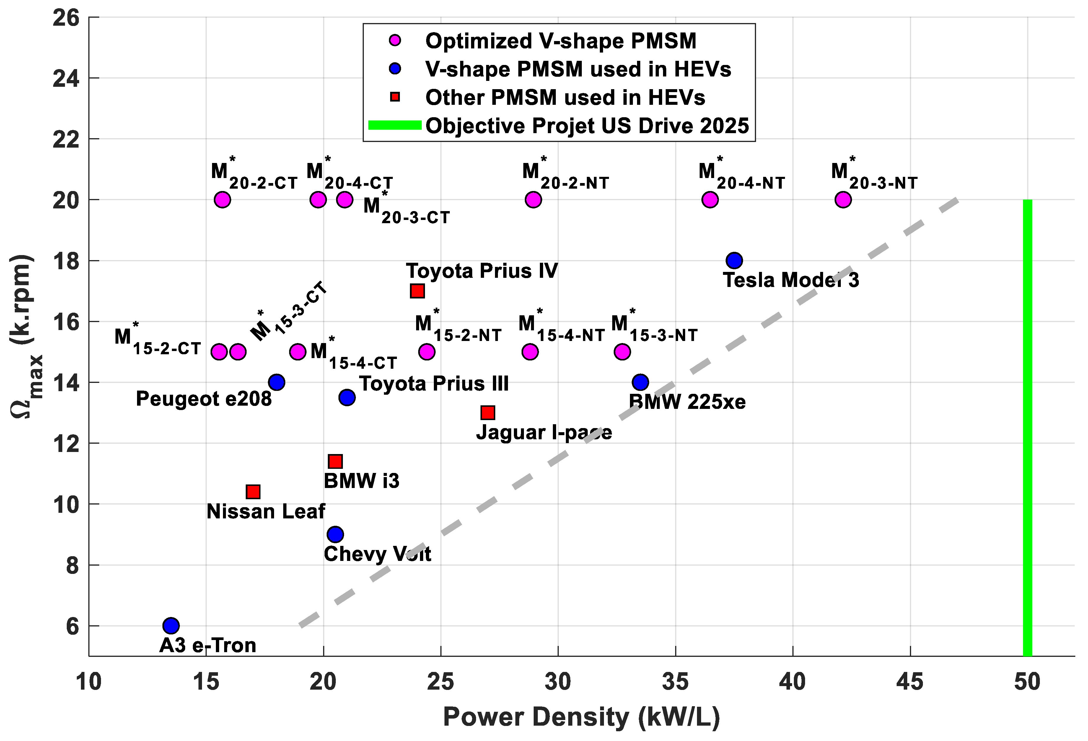
Figure 17 represents the optimized machines operating at the maximum rotational speed Ω m a x = 15,000   rpm and Ω m a x = 20,000   rpm , as well as other machines used in the automotive industry in the graph maximum speed–power density. 
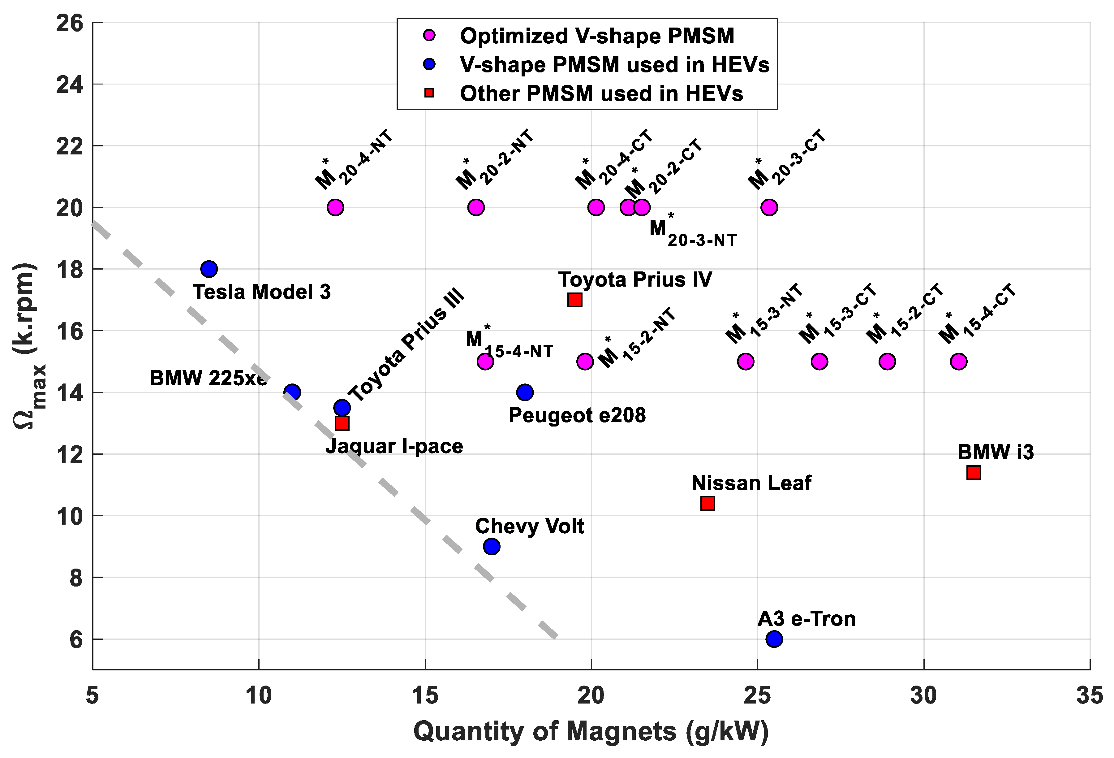
Figure 18 represents the same machines in the graph maximum speed–quantity of magnets per power.
Current ball bearings used in automobiles operate up to 20,000 rpm. Given this limitation, it is preferable to keep the maximum rotational speed below this limit, as recommended by the US Drive 2025 project, and to use new technologies to design a machine with high power density, which allows for avoiding problems related to bearings and vibrations. For this purpose, the machine with p = 3 is the best candidate achieving a power density of 42.14 kW/L, getting close to 50 kW/L, the objective fixed in the US Drive 2025 project. The gray dashed line in Figure 17 describes the correlation between power density and speed for existing and optimized electric machines. This evident and high correlation means increasing power is mainly done by increasing speed. The same observation is obtained with the gray dashed line in Figure 18, which represents the correlation between the amount of magnets and speed. Based on this correlation, decreasing the amount of magnets is mainly done by increasing speed. Machines near the dashed line in both graphs use new technologies, which means that the use of new technologies also helps increase the power density and decreases the amount of magnets. As mentioned before, it is possible to further improve power density and minimize magnets amount by increasing the DC voltage, equal to 500 V, in our work. New cooling techniques must be designed to evacuate significant losses generated in NT-based machines, such as oil spray on the end-windings region or oil injection into the stator slots, solutions adopted by Telsa and AVL [23]. The use of new technologies allows for reducing the amount of magnets (Figure 18) and, therefore, the cost of the machine. As mentioned previously, it is possible to further reduce the cost of the machine by using magnets without rare earth materials such as dysprosium (Dy) and terbium (Tb), a solution proposed by AVL [23]. In order to do so, it is essential to guarantee the good cooling of the machine to avoid the demagnetization of the magnets. A fine thermal analysis of the machine must therefore be carried out to achieve a high power density with a reasonable price, which would meet the ambitious objectives of the US Drive 2025 project in terms of power density (50 kW/L) and price of the machine (USD 3/kW).

6. Conclusions

In this work, one single V-shaped IPMSM is optimized based on similar specifications of the Peugeot e208′s machine. Results show that this machine achieves the required performances for electric vehicles for maximum rotational speed up to 40,000 rpm. Achieved performances show that, to obtain high power density, it is worth using new technologies and keeping the speed below 20,000 rpm to avoid problems related to the bearings' speed limitation and vibrations. Therefore, efforts must be made on the design of advanced cooling techniques, which require a fine thermal analysis of the machine. Besides, this will also prevent designing a gearbox with a very high transmission ratio. It is important to note that the optimal choice of the number of pole pairs allowing the lowest volume of the machine mainly depends on the maximum rotational speed and the technologies used. Losses due to circulating currents were not included in the optimization process. One solution that can be proposed to mitigate this effect is using a skewed stator or rotor. Future work will be focused on this solution and thermal analysis of machines with high power density.

Author Contributions

Writing—original draft preparation, T.E.H.; writing—review and editing, S.H., F.L., M.G., G.M.-R., and M.B. All authors have read and agreed to the published version of the manuscript.

Funding

This research was funded by “OpenLab Electrical Engineering for Mobility, Stellantis, France” and “Association Nationale de la Recherche et de la Technologie”.

Data Availability Statement

Not applicable.

Conflicts of Interest

The authors declare no conflict of interest.

References

  1. Li, S.; Li, Y.; Choi, W.; Sarlioglu, B. High-Speed electric machines: Challenges and design considerations. IEEE Trans. Transp. Electrific. 2016, 2, 2–13. [Google Scholar] [CrossRef]
  2. Schubert, E.; Li, S.; Sarlioglu, B. High-speed surface permanent magnet machines—Rotor design analysis, considerations, and challenges. In Proceedings of the 2016 IEEE Transportation Electrification Conference and Expo (ITEC), Dearborn, MI, USA, 27–29 June 2016; pp. 1–6. [Google Scholar] [CrossRef]
  3. Gallicchio, G.; Di Nardo, M.; Palmieri, M.; Marfoli, A.; Degano, M.; Gerada, C.; Cupertino, F. High speed synchronous reluctance machines: Modeling, design and limits. IEEE Trans. Energy Convers. 2022, 37, 585–597. [Google Scholar] [CrossRef]
  4. Shen, J.; Qin, X.; Wang, Y. High-speed permanent magnet electrical machines—Applications, key issues and challenges. CES Trans. Electr. Mach. Syst. 2018, 2, 23–33. [Google Scholar] [CrossRef]
  5. Belahcen, A.; Martin, F.; El-Hadi Zaim, M.; Dlala, E.; Kolondzovski, Z. Combined FE and Particle Swarm algorithm for optimi-zation of high speed PM synchronous machine. COMPEL Int. J. Comput. Math. Electr. Electron. Eng. 2015, 34, 475–484. [Google Scholar] [CrossRef]
  6. Belahcen, A.; Martin, F.; El-Hadi Zaim, M.; Dlala, E.; Kolondzovski, Z. Particle swarm optimization of the stator of a high speed PM synchronous machine. In Proceedings of the Digests of the 2010 14th Biennial IEEE Conference on Electromagnetic Field Computation, Chicago, IL, USA, 9–12 May 2010; p. 1. [Google Scholar] [CrossRef]
  7. Benlamine, R.; Hamiti, T.; Vangraefschepe, F. Design of 60 kW–35,000 rpm interior PM machine for automotive application. In Proceedings of the International Conference on Optimization of Electrical and Electronic Equipment (OPTIM) & Intl Aegean Conference on Electrical Machines and Power Electronics (ACEMP), Brasov, Romania, 25–27 May 2017; pp. 311–316. [Google Scholar] [CrossRef]
  8. Gao, P.; Sun, X.; Gerada, D.; Gerada, C.; Wang, X. Improved V-shaped interior permanent magnet rotor topology with inward-extended bridges for reduced torque ripple. IET Electr. Power Appl. 2020, 14, 2404–2411. [Google Scholar] [CrossRef]
  9. Zhang, G.; Yu, W.; Hua, W.; Cao, R.; Qiu, H.; Guo, A. The Design and Optimization of an Interior, Permanent Magnet Synchronous Machine Applied in an Electric Traction Vehicle Requiring a Low Torque Ripple. Appl. Sci. 2019, 9, 3634. [Google Scholar] [CrossRef] [Green Version]
  10. Yang, Y.; Castano, S.M.; Yang, R.; Kasprzak, M.; Bilgin, B.; Sathyan, A.; Dadkhah, H.; Emadi, A. Design and Comparison of Interior Permanent Magnet Motor Topologies for Traction Applications. IEEE Trans. Transp. Electrific. 2017, 3, 86–97. [Google Scholar] [CrossRef]
  11. Tang, N.; Brown, I.P. Comparison of Candidate Designs and Performance Optimization for an Electric Traction Motor Targeting 50 kW/L Power Density. In Proceedings of the IEEE Energy Conversion Congress and Exposition (ECCE), Vancouver, BC, Canada, 10–14 October 2021; pp. 3675–3682. [Google Scholar] [CrossRef]
  12. Kim, S.-E.; You, Y.-M. Optimization of a Permanent Magnet Synchronous Motor for e-Mobility Using Metamodels. Appl. Sci. 2022, 12, 1625. [Google Scholar] [CrossRef]
  13. Bernard, N.; Dang, L.; Olivier, J.-C.; Bracikowski, N.; Wasselynck, G.; Berthiau, G. Design optimization of high-speed PMSM for electric vehicles. In Proceedings of the 2015 IEEE Vehicle Power and Propulsion Conference (VPPC), Montreal, QC, Canada, 19–22 October 2015. [Google Scholar] [CrossRef]
  14. Soltani, M.; Nuzzo, S.; Barater, D.; Franceschini, G. A Multi-Objective Design Optimization for a Permanent Magnet Synchronous Machine with Hairpin Winding Intended for Transport Applications. Electronics 2021, 10, 3162. [Google Scholar] [CrossRef]
  15. Reddy, P.B.; Jahns, T.M.; Bohn, T.P. Transposition effects on bundle proximity losses in high-speed PM machines. In Proceedings of the 2009 IEEE Energy Conversion Congress and Exposition, San Jose, CA, USA, 20–24 September 2009; pp. 1919–1926. [Google Scholar] [CrossRef]
  16. Reddy, P.B.; Jahns, T.M. Analysis of bundle losses in high speed machines. In Proceedings of the The 2010 International Power Electronics Conference—ECCE ASIA, Sapporo, Japan, 21–24 June 2010; pp. 2181–2188. [Google Scholar] [CrossRef]
  17. Mellor, P.H.; Wrobel, R.; McNeill, N. Investigation of proximity losses in a high speed brushless permanent magnet motor. In Proceedings of the Conference Record of the 2006 IEEE Industry Applications Conference Forty-First IAS Annual Meeting, Tampa, FL, USA, 8–12 October 2006; pp. 1514–1518. [Google Scholar] [CrossRef] [Green Version]
  18. Fatemi, A.; Ionel, D.M.; Demerdash, N.A.; Staton, D.A.; Wrobel, R.; Chong, Y.C. A computationally efficient method for calculation of strand eddy current losses in electric machines. In Proceedings of the 2016 IEEE Energy Conversion Congress and Exposition (ECCE), Milwaukee, WI, USA, 18–22 September 2016; pp. 1–8. [Google Scholar] [CrossRef] [Green Version]
  19. El Hajji, T.; Hlioui, S.; Louf, F.; Gabsi, M.; Mermaz-Rollet, G.; Belhadi, M. Hybrid model for AC Losses in High Speed PMSM for arbitrary flux density waveforms. In Proceedings of the International Conference on Electrical Machines (ICEM), Virtual, 23–15 August 2020; pp. 2426–2432. [Google Scholar] [CrossRef]
  20. Leuning, N.; Jaeger, M.; Schauerte, B.; Stöcker, A.; Kawalla, R.; Wei, X.; Hirt, G.; Heller, M.; KorteKerzel, S.; Böhm, L.; et al. Material Design for Low-Loss Non-Oriented Electrical Steel for Energy Efficient Drives. Materials 2021, 14, 6588. [Google Scholar] [CrossRef] [PubMed]
  21. Mohamed, A.H.; Vansompel, H.; Sergeant, P. An Integrated Modular Motor Drive with Shared Cooling for Axial Flux Motor Drives. IEEE Trans. Ind. Electron. 2021, 68, 10467–10476. [Google Scholar] [CrossRef]
  22. Salameh, M.; Spillman, T.; Krishnamurthy, M.; Brown, I.P.; Ludois, D.C. Wound field synchronous machine with segmented rotor laminations and die compressed field winding. In Proceedings of the 2019 IEEE Energy Conversion Congress and Exposition (ECCE), Baltimore, MD, USA, 29 September–3 October 2019; pp. 1739–1746. [Google Scholar] [CrossRef]
  23. Deiml, M.; Eriksson, T.; Schneck, M.; Tan-Kim, A. High-speed Electric Drive Unit for the Next Generation of Vehicles. ATZ Worldw. 2019, 121, 42–47. [Google Scholar] [CrossRef]
  24. Cisse, K.M.; Hlioui, S.; Belhadi, M.; Mermaz Rollet, G.; Gabsi, M.; Cheng, Y. Design Optimization of Multi-Layer Permanent Magnet Synchronous Machines for Electric Vehicle Applications. Energies 2021, 14, 7116. [Google Scholar] [CrossRef]
  25. Van Millingen, R.D.; van Millingen, J.D. Phase shift torquemeters for gas turbine development and monitoring. In Proceedings of the ASME 1991 International Gas Turbine and Aeroengine Congress and Exposition, Orlando, FL, USA, 3–6 June 1991; pp. 1–10. [Google Scholar] [CrossRef] [Green Version]
  26. Kurvinen, E. Design and simulation of high-speed rotating electrical machinery. Ph.D. Thesis, Lappeenranta University of Technology, Lappeenranta, Finland, 2016. [Google Scholar]
  27. Benlamine, R.; Hamiti, T.; Vangraefschepe, F.; Lhotellier, D. Electromagnetic, Structural and Thermal Analyses of High-Speed PM Machines for Aircraft Application. In Proceedings of the XIII International Conference on Electrical Machines (ICEM), Alexandroupoli, Greece, 3–6 September 2018; pp. 212–217. [Google Scholar] [CrossRef]
  28. Rezzoug, A.; El-Hadi Zaïm, M.E. High-Speed Electric Machines. In Non-Conventional Electrical Machines; John Wiley and Sons: Hoboken, NJ, USA, 2013; pp. 117–189. [Google Scholar]
  29. Binder, A.; Schneider, T. High-speed inverter-fed AC drives. In Proceedings of the International Aegean Conference on Electrical Machines and Power Electronics (ACEMP), Bodrum, Turkey, 10–12 September 2007; pp. 9–16. [Google Scholar] [CrossRef]
  30. Bertotti, G. Physical interpretation of eddy current losses in ferromagnetic materials, I. theoretical considerations. J. Appl. Phys. 1985, 57, 2110–2117. [Google Scholar] [CrossRef]
  31. Ishak, D.; Zhu, Z.Q.; Howe, D. Eddy-current loss in the rotor magnets of permanent-magnet brushless machines having a fractional number of slots per pole. IEEE Trans. Magn. 2005, 41, 2462–2469. [Google Scholar] [CrossRef] [Green Version]
  32. Pyrhonen, J.; Jokinen, T.A.; Hrabovcova, V.A. Losses and Heat Transfer. In Design of Rotating Electrical Machines, 2nd ed.; John Wiley & Sons Ltd.: West Sussex, UK, 2014; pp. 527–529. [Google Scholar]
  33. Ramo, S.; Whinnery, J.R. Fields and Waves in Modern Radio; Wiley: New York, NY, USA, 1944. [Google Scholar]
  34. Sullivan, C.R. Computationally efficient winding loss calculation with multiple windings, arbitrary waveforms, and two-dimensional or three-dimensional field geometry. IEEE Trans. Power Electron. 2001, 16, 142–150. [Google Scholar] [CrossRef]
  35. Taran, N.; Rallabandi, V.; Ionel, D.M.; Heins, G.; Patterson, D. A Comparative Study of Methods for Calculating AC Winding Losses in Permanent Magnet Machines. In Proceedings of the 2019 IEEE International Electric Machines & Drives Conference (IEMDC), San Diego, CA, USA, 12–15 May 2019; pp. 2265–2271. [Google Scholar] [CrossRef]
  36. Gyselinck, J.; Sabariego, R.V.; Dular, P. Time-Domain Homogenization of Windings in 2-D Finite Element Models. IEEE Trans. Magn. 2007, 43, 1297–1300. [Google Scholar] [CrossRef] [Green Version]
  37. Volpe, G.; Popescu, M.; Marignetti, F.; Goss, J. Modelling AC Winding Losses in a PMSM with High Frequency and Torque Density. In Proceedings of the 2018 IEEE Energy Conversion Congress and Exposition (ECCE), Portland, OR, USA, 23–27 September 2018; pp. 2300–2305. [Google Scholar] [CrossRef]
  38. Ferreira, J.A. Appropriate modelling of conductive losses in the design of magnetic components. In Proceedings of the 21st Annual IEEE Conference on Power Electronics Specialists, San Antonio, TX, USA, June 1990; pp. 780–785. [Google Scholar] [CrossRef]
  39. Sato, Y.; Ishikawa, S.; Okubo, T.; Abe, M.; Tamai, K. Development of High Response Motor and Inverter System for the Nissan LEAF Electric Vehicle. In Proceedings of the SAE 2011 World Congress & Exhibition, Detroit, MI, USA, 11–14 April 2011; pp. 1–8. [Google Scholar] [CrossRef]
  40. Gu, W.; Zhu, X.; Quan, L.; Du, Y. Design and Optimization of Permanent Magnet Brushless Machines for Electric Vehicle Applications. Energies 2015, 8, 13996–14008. [Google Scholar] [CrossRef] [Green Version]
  41. Bobba, S.; Carrara, S.; Huisman, J.; Mathieux, F.; Pavel, C. Critical Raw Materials for Strategic Technologies and Sectors in the EU—A Foresight Study; European Commission: Brussels, Belgium, 2020. [Google Scholar] [CrossRef]
Figure 1. One pole of single-layer V-shaped IPMSM.
Machines 11 00057 g001
Figure 2. (a) Slot filled with real conductors used for DFEA model; (b) equivalent slot uniformly filled with conductor material and virtually placed conductors used for SFEA model.
Machines 11 00057 g002
Figure 3. 2D grid on the slot.
Machines 11 00057 g003
Figure 4. Geometry of the machine used for (a) SFEA model and (b) DFEA model.
Machines 11 00057 g004
Figure 5. Nearest grid’s node to the center of the virtual conductor.
Machines 11 00057 g005
Figure 6. Operating points used for optimization.
Machines 11 00057 g006
Figure 7. Flowchart of multiphysics design optimization methodology of high-speed machine.
Machines 11 00057 g007
Figure 8. Pareto front of all electric machines operating at Ω m a x = 15,000   rpm .
Machines 11 00057 g008
Figure 9. (a) M 15 2 C T * , (b) M 15 3 C T * , (c) M 15 4 C T * , (d) M 15 2 N T * , (e) M 15 3 N T * , (f) M 15 4 N T * , (g) Machine used in Peugeot e208.
Machines 11 00057 g009
Figure 10. Pareto front of all electric machines operating at Ω m a x = 20,000   rpm .
Machines 11 00057 g010
Figure 11. (a) M 20 2 C T * , (b) M 20 3 C T * , (c) M 20 4 C T * , (d) M 20 2 N T * , (e) M 20 3 N T * , (f) M 20 4 N T * , (g) Machine used in Tesla Model 3.
Machines 11 00057 g011
Figure 12. Pareto front of all electric machines operating at Ω m a x = 30,000   rpm .
Machines 11 00057 g012
Figure 13. (a) M 30 2 C T * , (b) M 30 3 C T * , (c) M 30 4 C T * , (d) M 30 2 N T * , (e) M 30 3 N T * , (f) M 30 4 N T * .
Machines 11 00057 g013
Figure 14. Pareto front of all electric machines operating at Ω m a x = 40,000   rpm .
Machines 11 00057 g014
Figure 15. (a) M 40 2 C T * , (b) M 40 3 C T * , (c) M 40 4 C T * , (d) M 40 2 N T * , (e) M 40 3 N T * , (f) M 40 4 N T * .
Machines 11 00057 g015
Figure 16. Characteristics of optimal CT-based machines: (a-1) Power density, (b-1) efficiency at points 1 and 2, (c-1) quantity of magnets, (d-1) quantity of copper; and Characteristics of optimal NT-based machines: (a-2) Power density, (b-2) efficiency at points 1 and 2, (c-2) quantity of magnets, (d-2) quantity of copper.
Machines 11 00057 g016
Figure 17. Maximum rotational speed vs. power density for optimal machines and other machines used in hybrid electric vehicles (HEV).
Machines 11 00057 g017
Figure 18. Maximum rotational speed vs. quantity of magnets per power for optimal machines and other machines used in hybrid electric vehicles (HEV).
Machines 11 00057 g018
Table 1. Definitions of high-speed machines in the literature.
DefinitionReference
Definition 1“Every time rotational speed occurs as a major constraint, either directly or indirectly, in the conception and design of the electric machine, we are referring to a high-speed machine”[28]
Definition 2 150   m / s < V p [26]
Definition 3 100   m / s < V p < 250   m / s [29]
Definition 4 Ω > 10,000   rpm & D Ω > 10 5 [25]
Table 2. Geometric parameter of single-layer V-shaped IPMSM.
Electric MachineParameters
StatorSlot5 parameters *
Outer radius R o u t , s
Inner radius R i n n , s
RotorPM5 parameters *
Air holes (near PM)5 parameters *
Air gap length δ
Outer radius R o u t , r = R i n n , s δ
Inner radius R i n n , r
Active Length l a c t
Operating Point P i Current density J i
Control angle ψ i
* Parameters of slot, PM, and air holes can be found in [24].
Table 3. Electric vehicle specifications of electric machine optimization.
QuantityValue
Maximum Power: P m a x ( kW ) 100
Flux Weakening Ratio: k Ω 4
Maximum Rotational Speed: Ω m a x ( r p m ) 15,000
20,000
30,000
40,000
Torque at Point 1: T P 1 ( N . m ) -
Torque at Point 2: T P 2 ( N . m ) -
Maximum Torque Ripple at Point 1 (%)30
Maximum Torque Ripple at Point 2 (%)50
Number of Pole Pair: p 2
3
4
Fill Factor K f i l l (%)45
65
Lamination Thickness T h l a m ( m m ) 0.35
0.25
Remanent Flux Density of PM: B r ( T ) 1.2
Maximum Current Density: J m a x ( A r m s / m m ² ) 15
33
Number of Slots per Pole per Phase: spp2
Air Gap Length (mm)0.7
DC   Voltage :   V D C ( V ) 500
Maximum Current per Phase: I p h m a x ( A r m s ) 445
WindingsDistributed—Series
Yield Strength (MPa)400
Table 4. Parameters value of both classic and new technologies.
ParameterType of Technology
Classic TechnologiesNew Technologies
Fill Factor45%65%
Maximum Current Density15 Arms/mm²33 Arms/mm²
Lamination Thickness0.35 mm0.25 mm
Table 5. Performances and characteristics of optimal machines operating at Ω m a x = 15,000   rpm and machine used in Peugeot e208.
M 15 2 C T * M 15 3 C T * M 15 4 C T * M 15 2 N T * M 15 3 N T * M 15 4 N T * Peugeot
e208
p 2342344
P m a x ( k W ) 100100100100100100100
Ω m a x ( r p m ) 15,00015,00015,00015,00015 00015,00014,000
P v o l ( k W / L ) 15.516.318.924.432.728.818
PM/P28.926.83119.824.616.818
Copp/P9279.868.642.233.230.4-
R o u t s 95.397.689.279.374.382.295
L a c t 189176.8190.4182.7162.2152.9175
T h l a m 0.350.350.350.250.250.250.35
K f i l l 454545656565~65
J m a x 15151533333316
I p h m a x 445445445445445445370
V D C 500500500500500500350
Type of windingDSWDSWDSWDSWDSWDSWDHW
I 1 ,   I 2 380/199407/234435/257407/195428/229429/215-
J 1 ,   J 2 14.3/7.514/8.114/8.331.7/15.231/16.627.2/13.9-
N t u r n s 5325324
R p h 138.66.722.315.111.1
n s h 3950475265701
d s h 0.90.850.90.560.520.53-
η 1 ,   η 2 94.4/95.295.5/95.995.9/9689.9/96.792.2/96.694.3/96.8-
P J 1 ,   P J 2 5655/15594294/14213801/133211,109/25528345/23925845/1537-
P I 1 ,   P I 2 270/2758344/1627435/1978159/545193/686263/1074-
P A C 1 ,   P A C 2 27/8525/14055/3729/409/4412/41-
P M 1 ,   P M 2 35/63745.6/86234/61018/30023/39038/727-
Table 6. Performances and characteristics of optimal machines operating at Ω m a x = 20,000   rpm and machine used in Tesla Model 3.
M 20 2 C T * M 20 3 C T * M 20 4 C T * M 20 2 N T * M 20 3 N T * M 20 4 N T * Tesla Model 3
p 2342343
P m a x ( k W ) 100100100100100100202
Ω m a x ( r p m ) 20,00020,00020,00020,00020,00020,00018,000
P v o l ( k W / L ) 15.72119.82942.136.537.5
PM/P21.125.420.116.521.512.318
Copp/P86.953.360.73927.732.9-
R o u t s 96.883.288.171.263.768.8110.3
L a c t 178.2197.7187.4194.2173.8173.2131
T h l a m 0.350.350.350.250.250.250.25
K f i l l 45454565656545
J m a x 15151533333333.7
I p h m a x 445445445445445445850
V D C 500500500500500500350
Type of windingDSWDSWDSWDSWDSWDSWDSW
I 1 ,   I 2 392/205442/235415/219412/205378/256419/219-
J 1 ,   J 2 12/6.315/812.8/6.727.9/13.833/22.325.9/13.5-
N t u r n s 42243215
R p h 7.85.85.715.51810.9-
n s h 49504867548919
d s h 10.8510.530.520.480.75
η 1 ,   η 2 96.1/96.496.3/9696.5/95.292.5/96.992.6/95.294.3/96.3-
P J 1 ,   P J 2 3610/9893378/9592936/8197921/19567828/35915791/1583-
P I 1 ,   P I 2 438/1887468/2176584/3000215/807211/837289/1591-
P A C 1 ,   P A C 2 31/15029/13391/45212/4512/9518/77-
P M 1 ,   P M 2 39/74251/101044/84926/47430/56843/835-
Table 7. Performances and characteristics of optimal machines operating at Ω m a x = 30,000   rpm and machines designed by AVL [23].
M 30 2 C T * M 30 3 C T * M 30 4 C T * M 30 2 N T * M 30 3 N T * M 30 4 N T * AVL [23]
p 2342343
P m a x ( k W ) 100100100100100100150
Ω m a x ( r p m ) 30,00030,00030,00030,00030,00030,00030,000
P v o l ( k W / L ) 25.227.824.853.448.157.745.5
PM/P18.912.915.610.67.912.5-
Copp/P60.148.557.130.13422.3-
R o u t s 74.772.587.25463.654.475
L a c t 196197146.6188151.2179.2175
T h l a m 0.350.350.350.250.250.250.2
K f i l l 454545656565-
J m a x 151515333333>15
I p h m a x
( A r m s )
445445445445445445525
V D C ( V ) 500500500500500500800
Type of windingDSWDSWDSWDSWDSWDSWDSW
I 1 ,   I 2 444/212421/209439/214414/196423/193371/217-
J 1 ,   J 2 14.5/6.915/7.413.6/6.632.1/15.226.2/1232/18.7-
N t u r n s 322432-
R p h 5.885.725.3516.211.4714.6-
n s h 474848608959-
d s h 0.90.850.90.520.480.5-
η 1 ,   η 2 96.2/96.196.4/94.496/94.392.2/96.694/96.894.1/96.192/93
P J 1 ,   P J 2 3480/7923053/7513100/7348333/18746168/12866040/2073-
P I 1 ,   P I 2 447/1989613/3619874/3182186/1111288/1156288/1092-
P A C 1 ,   P A C 2 33/12075/263171/75616/5126/9538/224-
P M 1 ,   P M 2 56/115070/148770/157132/60539/79241/829-
Table 8. Performances and characteristics of optimal machines operating at Ω m a x = 40,000   rpm .
M 40 2 C T * M 40 3 C T * M 40 4 C T * M 40 2 N T * M 40 3 N T * M 40 4 N T *
p 234234
P m a x ( k W ) 100100100100100100
Ω m a x ( r p m ) 40,00040,00040,00040,00040,00040,000
P v o l ( k W / L ) 30.32525.55263.968.2
PM/P13.411.612.78.99.46
Copp/P42.643.332.421.721.823
R o u t s 74.5807558.55052.2
L a c t 158.6183.6210162.8188.3163.5
T h l a m 0.350.350.350.250.250.25
K f i l l 454545656565
J m a x 151515333333
I p h m a x 445445445445445445
V D C ( V ) 500500500500500500
Type of windingDSWDSWDSWDSWDSWDSW
I 1 ,   I 2 370/256423/215443/224429/208445/194423/195
J 1 ,   J 2 14/9.714.4/7.314.2/7.232/15.531.7/13.932.4/15
N t u r n s 321322
R p h 6.45.33.410.69.811.9
n s h 384745747772
d s h 0.90.850.90.480.480.48
η 1 ,   η 2 96.9/92.696.3/95.396.8/9394.2/96.694.2/96.893.6/95.7
P J 1 ,   P J 2 2620/12562880/7432026/5185858/13765802/11126394/1361
P I 1 ,   P I 2 520/5156895/27581072/4668303/1076364/1036449/1788
P A C 1 ,   P A C 2 54/462121/590123/57217/6536/13580/341
P M 1 ,   P M 2 77/176858/124889/200049/106749/102849/1062
Disclaimer/Publisher’s Note: The statements, opinions and data contained in all publications are solely those of the individual author(s) and contributor(s) and not of MDPI and/or the editor(s). MDPI and/or the editor(s) disclaim responsibility for any injury to people or property resulting from any ideas, methods, instructions or products referred to in the content.

