Dimensionality Reduction Methods of a Clustered Dataset for the Diagnosis of a SCADA-Equipped Complex Machine

Abstract

Machinery diagnostics in the industrial field have assumed a fundamental role for both technical, economic and safety reasons. The use of sensors, data collection and analysis has increasingly advanced to investigate the health of machinery, predict the presence of faults and recognize their nature. The amount of data necessary for this purpose means that it is often necessary to implement dimension reduction methods to pre-process the useful features for the classification. Furthermore, the use of a multi-class dataset could involve data clustering in its multi-dimensional space. This study proposes a novel dimensionality reduction method, consisting of the combination of two different techniques. It aims at improving the quality of the features and, consequently, the classification performance with high-dimension clustered datasets. In addition, a case study is analyzed thanks to the data published by the Prognostics and Health Management Europe (PHME) society on the Data Challenge 2021. The results show an excellent recognition of the machine state of health both in terms of damage detection and identification. The performance indices also show an improvement in classification compared to other dimension reduction methods.

1. Introduction

In the industrial field, machine diagnostics has assumed an important role both because it allows the quality of products to be improved and because it permits a significantly reduction in maintenance costs and machine downtimes. It is also for this reason that data-based monitoring techniques are rapidly evolving. Maintenance is moving from corrective (run-to-failure) and preventive approaches to condition-based monitoring techniques (i.e., predictive maintenance). In addition to investigating the diagnostics and prognostics of industrial systems, many studies have recently focused not only on damage identification but also on damage recognition (i.e., prescriptive maintenance). Prescriptive maintenance requires a considerable amount of data to identify the type of arisen defects. The dimensionality of the dataset—especially in terms of the number of features—tends consequently to take on substantial sizes. In addition to this criticality, it is often difficult to record data during the operation of the machinery in the presence of defects (actual or simulated). Indeed, while the class inherent to the healthy condition usually contains many elements, the damages are expensive and difficult to obtain, as well as to diversify. Finally, since the training dataset includes acquisitions related to different machinery conditions, it is likely that, following an appropriate pre-processing, the data are grouped into clusters within a multidimensional space. All these characteristics could potentially further complicate the analysis since the use of some classification techniques (usually adopted in similar cases) is not optimal for datasets with the aforementioned properties. Therefore, proper pre-processing of this typology of data [1] is all the more fundamental to improve their quality and to apply clustering and classification techniques. It is also significant to adopt noise reduction techniques, to decrease the number of irrelevant variables and to minimize the cardinality of the set of features. These procedures allow the effects of the curse of dimensionality [2], the time requirements and the computational effort to be reduced.

The above arguments highlight the importance of Dimensionality Reduction Methods (DRMs) and the literature presents several techniques to achieve a feature space reduction. Huang et al. analyzed and classified the classical techniques for dimensionality reduction in [3], while the authors of [4] and [5] explored linear and nonlinear DRMs, respectively. Some of the techniques known in the literature were compared according to their speed and accuracy in [6]. Instead, Nguyen et al. [7] introduced guidelines for the correct application of DRMs and the interpretation of the related results. Among the most commonly known DRMs, it is worth mentioning the Principal Component Analysis (PCA) [8,9], the Kernel Dimensionality Reduction [10] and the Kernel PCA [11]. Feature selection methods—such as wrapper, embedded, filter and outlier detection methods [12]—exist in addition to DRMs. Nevertheless, while the features selection has the purpose of choosing the best features among those of the original space (without creating new features, but eliminating the dependent variables), the features reduction allows a novel space with reduced dimensionality to be obtained through original features combinations. In addition to the described techniques, the Novelty Indices (NIs), obtainable by applying the Novelty Detection (ND) could also be considered as a feature space with a reduced dimensionality. Among the existing diagnostic techniques of mechanical systems [13,14,15,16,17] present in the literature, the Novelty Detection is a classification method which aims to recognize the abnormal values. The latter values are directly correlated to fault detection of a generic industrial system when the confounding factors are excluded. Some examples of a ND-based diagnostic technique for prescriptive maintenance have been proposed in [18,19,20,21,22]. In particular, the study in [22] highlighted how such ND-based diagnostic techniques can also be used as DRMs. However, these existing dimensionality reduction techniques include some limitations (e.g., the over-positioning of clusters for the PCA and the absence of an angular reference of NIs calculated thanks to the Mahalanobis distance).

This study introduces a novel DRM that allows datasets to be pre-processed with the above-described characteristics (i.e., high dimensionality in terms of features, grouping into clusters and potentially, insufficient abnormal condition data). The proposed method could be decomposed into two complementary techniques which provide a multivariate space reduction. The first phase consists of a modified PCA for clusters recognition, which is named Clusters Component Analysis (CCA) hereafter. The second additional phase—which allows nonlinear behaviors to be included—is based on Novelty Indices (NIs) calculated through the Mahalanobis Distance (MD). These techniques are based on widely known and used methods (such as PCA and ND through an MD-based index). In addition to reducing the dimensionality in terms of features, they also aim at overcoming some limitations of the above techniques. The first CCA phase is essential to subsequently compute MD-based indices. Indeed, a dimensionality reduction is required when dealing with the covariance matrix, such as in the computation of Mahalanobis distances. The most common issue is obtaining a singular covariance matrix due to an excessive number of features compared to the available samples. However, a traditional PCA application may result in an inadequate pre-processing for certain datasets. In fact, in the literature there are several studies in which alternative methods to PCA or PCA modifications have been proposed to adapt and optimize the technique to specific cases. For instance, Ebeling et al. [23] proposed a combined cluster and principal component analysis to reduce data complexity. Ding et al. [24] developed an adaptive dimension reduction method, focusing on Expectation-Maximization (EM) and the K-means algorithm.

In principle, the combination of the proposed methods can be applied to any high-dimensional clustered dataset and is not restricted to any specific field. Future work will be dedicated to numerically verify the performance of the procedure with other datasets. Nevertheless, their application to a case study—related to the diagnostics and health monitoring of an industrial system—is presented and demonstrated. In particular, the Prognostics and Health Management Europe (PHME) society [25] has published a dataset on the Data Challenge 2021 [26] which is used as a reference. In addition to showing the applicability of these techniques, this dataset is used to validate the proposed models. For this purpose, the performance indices described in [22] and obtained through five different types of classifiers [27,28] are used as a reference. The final comparison between the proposed and the existing methods shows the accuracy improvements that each phase generates when the dataset presents clustered data.

The article is structured as follows. Section 2 recalls the test bench and dataset description. Section 3 reports the most relevant DRMs existing in the literature and on which the proposed techniques are based. Section 4 describes the proposed methodology for each approach. Finally, the results and conclusions are reported in Section 5 and Section 6, respectively.

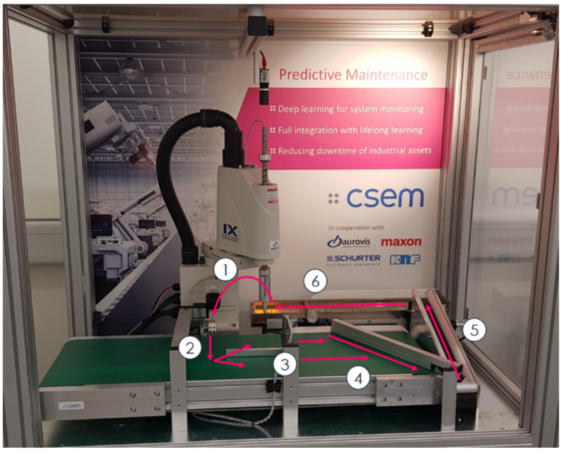
2. Test Bench and Dataset Description

The proposed DRM was developed as a general-purpose method with high-dimension clustered dataset conditions. The dataset distributed for the Prognostics and Health Management Europe (PHME) society Data Challenge 2021 [26] was used to validate the proposed models both because it satisfies the mentioned conditions of application, and because the comparison with the reference method turned out to be more understandable.

PHME’s dataset contains signals of a different nature related to a real industrial system—shown in Figure 1—for the quality control of electronic components. A 4-axis SCARA robot is the main component of the quality control line under analysis. Its diagnostics are possible thanks to the implementation of a Supervisory Control And Data Acquisition (SCADA) system. Recently, several SCADA datasets have become available for scientific purposes thanks to the growth of the attitude to these data. Natili et al. analyzed several pros and cons of using SCADA systems for fault diagnosis in [29]. The current SCADA system is composed of 50 sensors. These sensors record signals to monitor the machinery state of health in real-time. The complexity and heterogeneity of the systems in question makes the features extraction and the space dimensions reduction more challenging.

The recorded dataset contains 50 acquisition channels. Each of them refers to a time window equal to 10 s and is described through some specific characteristics ($vCnt$ = number of samples recorded; $vFreq$ = Sampling frequency; $vMax$ = Maximum recorded value; $vMin$ = Minimum recorded value; $vTrend$ = trend of the historical series and $value$ = Average value). Each of the 70 performed tests (50 tests concerned healthy conditions, while five conditions with different failures had a cardinality of four each) lasts from 1 to 3 h approximately. A proper pre-processing of the data collected during these experiments allowed a final $\mathit{X}$ matrix of size $m \times n$ and rank $L<=min\left(m,n\right)$, to be obtained where $m=70$ represents the total number of tests and $n=240$ columns is the number of features. The data included in the $\mathit{X}$ matrix was standardized on the mean value and on the standard deviation of the healthy class. Vector $C$ of size $1 \times m$ contains the labels and describes the condition of the machinery per each test. In the following, the convention whereby Class 0 indicates healthy conditions of the machinery is adopted. On the other hand, the various damages are defined as Class k, where $k$ enumerates the types of damage.

To conclude, the proposed methods were applied to the $\mathit{X}$ matrix in order to reduce its initial size $m \times n$. It is worth noting that the proposed DRM is relevant when $n>k$. Please refer to [22] for a more detailed description of the test bench and the structure of the dataset.

3. Existing Dimensionality Reduction Methods

This section contains brief references to the techniques on which the novel DRM proposed in this study is based. PCA and MD are mentioned with their limitations inherent to the case study.

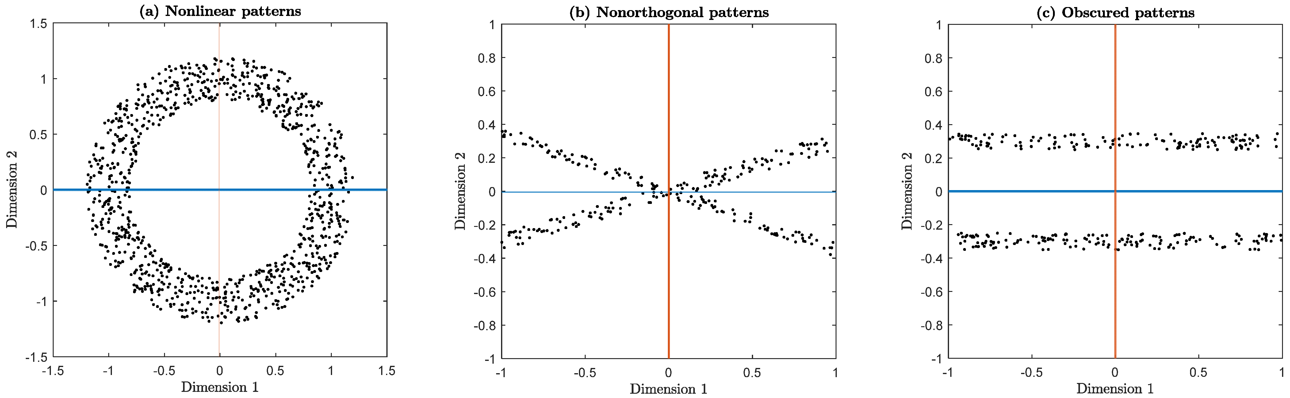
3.1. Linear DRM: Principal Component Analysis

Principal component analysis is a multivariate statistical technique used in numerous disciplines to analyze and extract relevant information from confusing data arrays. PCA gives the possibility to reduce the dimensionality of data systems, usually described by various inter-correlated variables. Its main objective is to reduce the complexity of high-dimensional data by expressing their information through new orthogonal variables, called Principal Components (PCs) and which act as weighted averages of the features. It is worth recalling that the PCs of our mean centered dataset $\mathit{X}$ are the eigenvectors of the covariance matrix $\Sigma$, mathematically defined as:

$$\Sigma =\frac{1}{n-1}\mathit{X}{\mathit{X}}^T$$

(1)

.

The solution of the eigenproblem corresponds to:

$$\Sigma \mathit{A}=\mathit{A}\Lambda$$

(2)

where $\mathit{A}$ is the $m\times m$ orthogonal matrix whose columns are the eigenvectors and $\Lambda$ is the diagonal matrix containing the $m$ eigenvalues ${\lambda }_j$ of the covariance matrix (usually sorted with descending magnitude).

In addition to its predominant function of selecting features and simplifying the dataset, PCA can also be considered as an unsupervised learning method similar to clustering. For these reasons, PCA is probably the most popular multivariate statistical analysis [30].

However, although the PCA greatly helps the analysis and interpretation of data, it does not always allow patterns to be correctly recognized. As highlighted in [31], PCA also has some limitations due to its assumptions. The main limitations are shown in Figure 2 and are (a) the difficulties in recognizing nonlinear data models, (b) the inability to recognize nonorthogonal patterns and (c) the over-positioning of obscured clusters. Furthermore, even in the favorable cases, there may still be open problems such as the choice of the number of components to consider. Although in [28] there are some guidelines to solve this issue—such as the identification of a threshold with respect to the eigenvalues of the covariance matrix calculated through the elbow test or equal to their average value—a lot of important information could be ignored.

Finally, since PCA exploits the covariance matrix $\Sigma$, any outlier could influence its performance. Analogously, the heteroscedasticity (i.e., the variance between the variables is significantly different) could also affect PCA results.

Section 4.1 proposes an alternative analysis specifically adopted to solve the limitations concerning the recognition of the clusters characterizing PCA. The aim of this method is the maximization of cluster recognition in cases where traditional PCs are not performing well. In addition to allowing a dimension reduction of data through a linear combination of features, this technique also aims at recognizing the optimal number of required features (considering a training dataset) and at minimizing the relative loss of information. In the application example below, this alternative PCA is used as a supervised learning method.

3.2. Nonlinear DRM: Mahalanobis Distance

The Mahalanobis distance is a measure based on the correlations between features, a characteristic that distinguishes it from Euclidean distance. The MD calculated in the space of the original variables considers the covariance matrix of the dataset of interest. In particular, the Mahalanobis distance of a centered dataset $\mathit{X}$ is defined as:

$$MD\left(\mathit{X}\right)=\sqrt{{\mathit{X}}^T{\Sigma }^{-1}\mathit{X}}$$

(3)

The multi-collinearity of the dataset (i.e., the high dimensionality of the data matrix in terms of potentially correlated and redundant features) causes the calculation of a singular (or almost singular) covariance matrix. For this reason, a dimension reduction through features selection or combination is usually necessary before the MD calculus. In addition to this problem regarding the inversion of the covariance matrix, MD is affected by the same PCA limitations. Indeed, MD is not able to properly distinguish nonlinear, nonorthogonal and obscured patterns and—at the same time—is influenced by outliers and heteroscedastic dataset. As part of pattern recognition, MD can be used as input for further classification and clustering techniques, as shown in [22,32].

Moreover, the novelty indices based on the MD have a further limitation. Since it is a distance, a single MD-based NI does not allow the recognition of the angular positioning of data within a multidimensional space, thus confusing some of them or potentially some clusters. Figure 5 precisely shows this aspect through an exemplary representation of a multivariate space containing three approximately equally spaced clusters. In particular, the chart representing the MD calculated with respect to Class 0 does not allow the data belonging to Classes 1 and 2 to be distinguished, although they are easily identifiable in the multivariate space. This is precisely the consequence of the highlighted limitation. One of the proposed methods uses the MD and aims at reducing the dimensionality of the dataset without losing this angular information and, consequently, at improving the classification model.

4. Proposed Methodology

This section presents the methodology adopted for each phase of the proposed technique to reduce the dimensionality of the data. A flowchart is presented in Figure 3 to summarize and clarify the proposed method. The described procedures are applied to the case study in Section 5.

It should be noted that—in the context of the diagnostics and health monitoring of mechanical systems—data are generally collected using suitable sensors (e.g., accelerometers, load cells and temperature sensors) positioned on the machinery of interest both during its operation in optimal conditions and with the presence of (alternatively simulating) faults, defects, damages and failures. Therefore, each performed test is classified through a specific label describing the condition of the machinery.

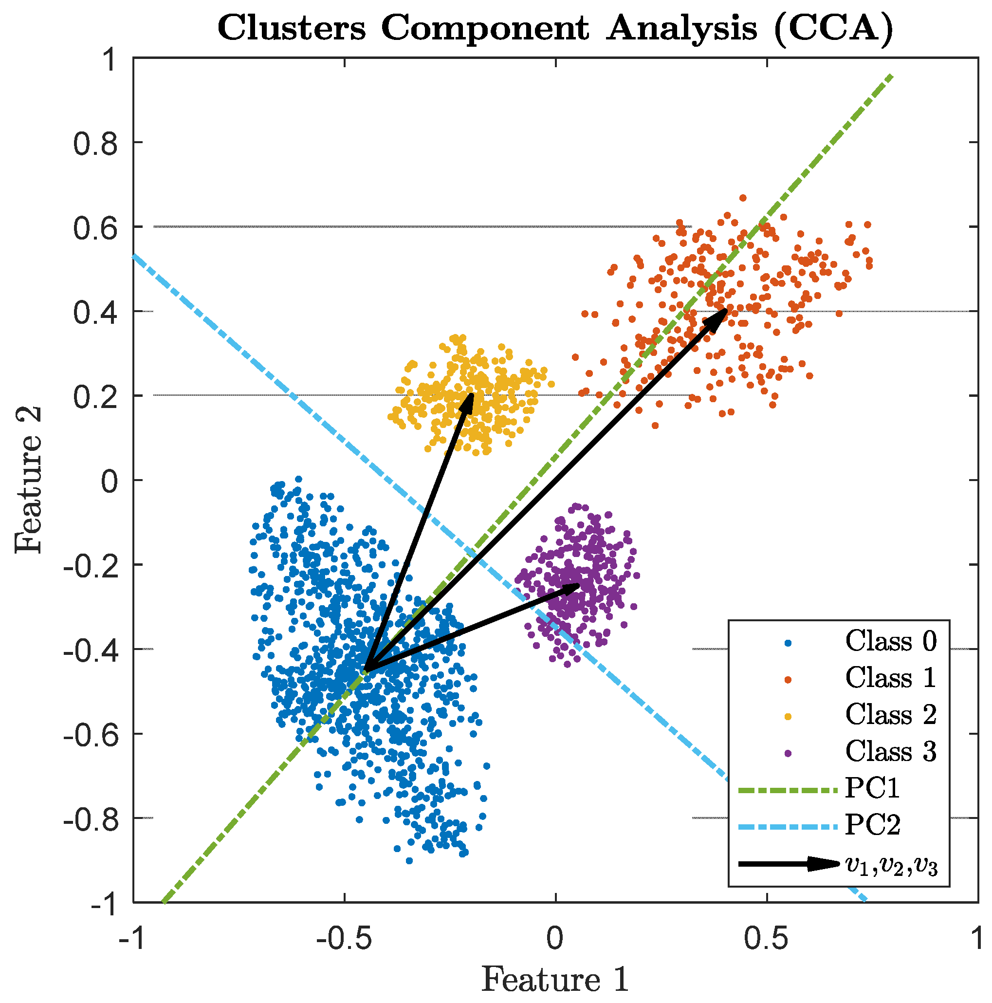
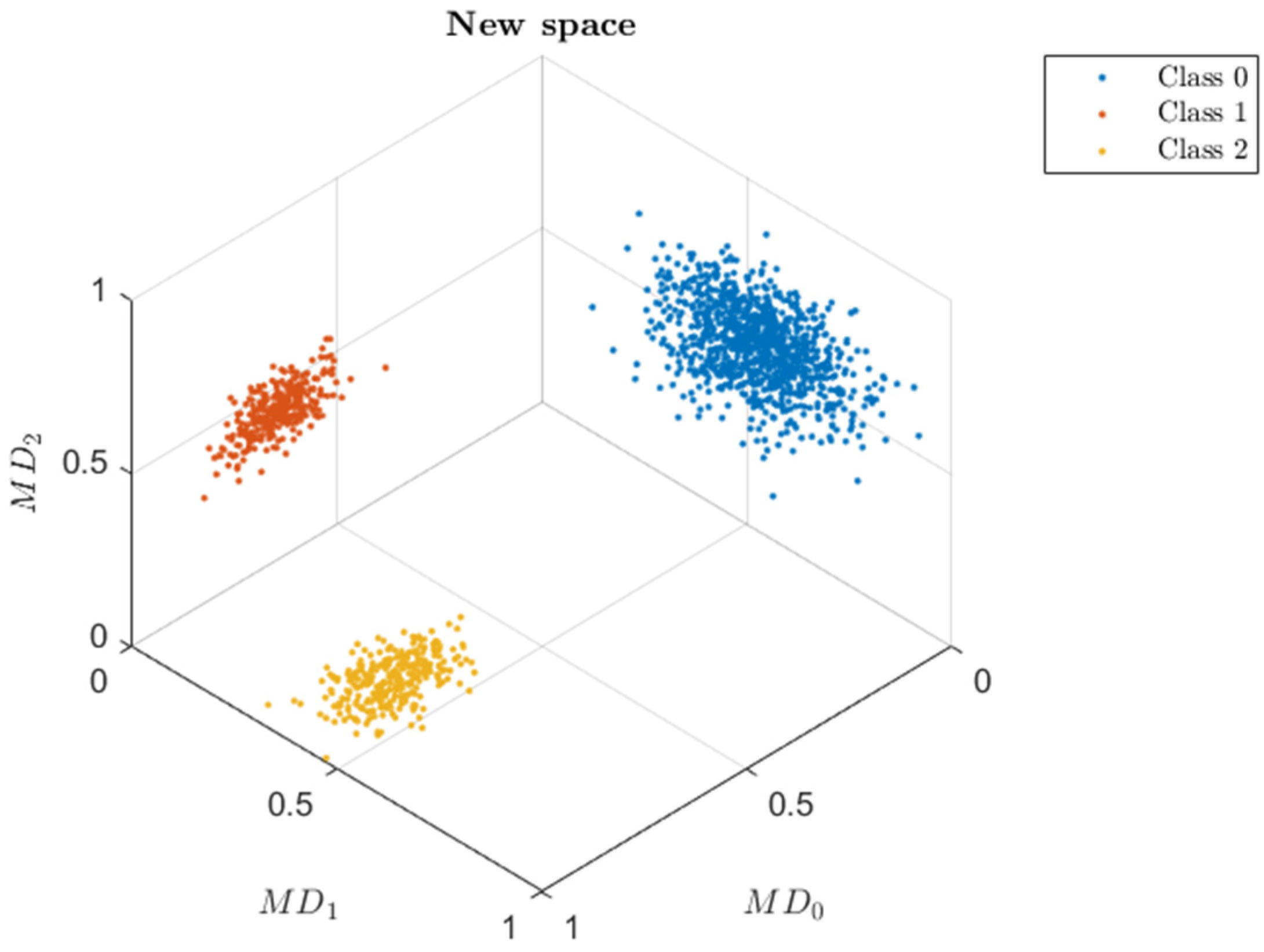
4.1. Clusters Component Analysis (CCA)

The main objective of this novel method is to reduce the size of the multivariate data matrix while minimizing the loss of information and, above all, allowing the recognition of clusters, which could be confused by PCA in particular conditions.

First of all, to reduce the outlier influence, it would be advisable to identify the outliers related to each class by means of a Hampel filter [33], which replaces the detected values with the median. In this way, the outliers are identified locally (according to the distribution of data per each class) rather than globally (considering the entire dataset). It allows false outlier removal to be avoided, caused by classes characterized by high recorded values, or not identifying them all correctly.

If the variance between the variables is significantly different or if unalike quantities or units of measurement are used, standardization may be required. Moreover, since the measured variables could differ significantly between classes, it is important to normalize the data with respect to Class 0. In this way, the set of data referring to the healthy condition of the machinery is centered with respect to the reference system of the $n$-dimensional space. The choice of standardizing all data with respect to Class 0 relies on the fact that healthy conditions are the reference in terms of machinery diagnostics.

To ensure that clusters, representing the test classes with damages, are arranged in a multidimensional space in such a way as to maximize their separation and facilitate their recognition, it is necessary to calculate the $n$-dimensional ${\mathit{v}}_k$ vectors (represented in Figure 4) that connect the centers of the Classes k clusters with the center of the Class 0 cluster (i.e., the origin of the reference system).

The $\left(k-1\right)n$ size matrix $\mathit{V}$, containing ${\mathit{v}}_k$ vectors, could allow transforming initial data from $R^n\to R^k$:

$$\mathit{Y}=\mathit{V}{\mathit{X}}^T$$

(4)

where $\mathit{Y}$ is a $\left(k-1\right)m$ matrix and represents a new set of data obtained as a combination of features, which can be geometrically interpreted as a projection of the initial points along the ${\mathit{v}}_k$ vectors. In this way, data representing the $m$ tests belong to a (k − 1)-dimensional space (reduced with respect to the initial $n$-dimensional space if $k<n-1$). In addition to the dimension reduction of the dataset, the loss of information resulting from this transformation is theoretically zero, as each initial $n$ feature contributes with a different weight to the creation of the new features contained in $\mathit{Y}$.

However, despite minimizing the loss of information, the contribution of some initial features could be redundant, as their projection would be considered on more vectors ${\mathit{v}}_k$. It is necessary to make the ${\mathit{v}}_k$ vectors orthogonal to each other to solve this redundancy of contributions and subsequently normalize them to avoid the stretch effects of the new (k − 1)-dimensional space. For this purpose, the Gram–Schmidt algorithm [34] was adopted. It allows a set of orthogonal unit vectors starting from a generic set of linearly independent vectors to be obtained. Numbering the vectors ${\mathit{v}}_k$ by sorting them in descendent magnitude (e.g., ${\mathit{v}}_1$ is the vector connecting the farthest cluster with respect to the health one), the projection of the i-th vector ${\mathit{v}}_i$ on ${\mathit{v}}_k$ is defined as:

$$pro{j}_{{\mathit{v}}_k}\left({\mathit{v}}_i\right)=\frac{⟨{\mathit{v}}_i,{\mathit{v}}_k⟩}{⟨{\mathit{v}}_k,{\mathit{v}}_k⟩}{\mathit{v}}_k$$

(5)

where $⟨,⟩$ is the scalar product. An orthonormal basis can be obtained by iterating the following calculations for each vector of the $\mathit{V}$ matrix:

$$\begin{array}{ccc}{\mathit{u}}_1={\mathit{v}}_1& ;& {\mathit{e}}_1=\frac{{\mathit{u}}_1}{\Vert {\mathit{u}}_1\Vert }\end{array}$$

(6)

$$\begin{array}{ccc}{\mathit{u}}_2={\mathit{v}}_2-pro{j}_{{\mathit{u}}_1}\left({\mathit{v}}_2\right)& ;& {\mathit{e}}_2=\frac{{\mathit{u}}_2}{\Vert {\mathit{u}}_2\Vert }\end{array}$$

(7)

$$\begin{array}{ccc}{\mathit{u}}_3={\mathit{v}}_3-pro{j}_{{\mathit{u}}_1}\left({\mathit{v}}_3\right)-pro{j}_{{\mathit{u}}_2}\left({\mathit{v}}_3\right)& ;& {\mathit{e}}_3=\frac{{\mathit{u}}_3}{\Vert {\mathit{u}}_3\Vert }\end{array}$$

(8)

$$\begin{array}{ccc}{\mathit{u}}_k={\mathit{v}}_k-{\displaystyle \sum _{j=1}^{k-1}} pro{j}_{{\mathit{u}}_j}\left({\mathit{v}}_k\right)& ;& {\mathit{e}}_k=\frac{{\mathit{u}}_k}{\Vert {\mathit{u}}_k\Vert }\end{array}$$

(9)

where $\left\{{\mathit{u}}_k\right\}$ is the orthogonal base obtained from $\left\{{\mathit{v}}_k\right\}$ and $\left\{{\mathit{e}}_k\right\}$ the orthonormal one. The new transformation from $R^n\to R^k$ is described by the $\mathit{E}$ matrix with $\left(k-1\right)\times n$ dimensions and containing orthogonal versors ${\mathit{e}}_k$:

$${\mathit{Y}}_o=\mathit{E}{\mathit{X}}^T$$

(10)

Consequently, it is possible to eliminate the redundancy of information present in the transformed data and contained in $\Sigma$ thanks to the orthogonalization of the $\left\{{\mathit{v}}_k\right\}$ vectors. Therefore, it is possible to perform an automatic features selection of the initial data, passing from $n$ to $k-1$ features. The diagnostic information lost in this transformation is minimal since the new features contained in ${\mathit{Y}}_0$ are a linear combination of the original ones, contained in $\mathit{X}$. After calculating the appropriate transformation matrix $\mathit{E}$ on the training dataset, it is possible to use the same transformation on a validation dataset or on data extracted and processed in real-time to correctly classify the operating condition of a specific machine. It is worth noting that the proposed CCA could be considered similar to PCA since both of them provide a reduced orthogonal space. However, CCA initially considers the vectors connecting the centers of clusters instead of the maximum variance directions as PCA does.

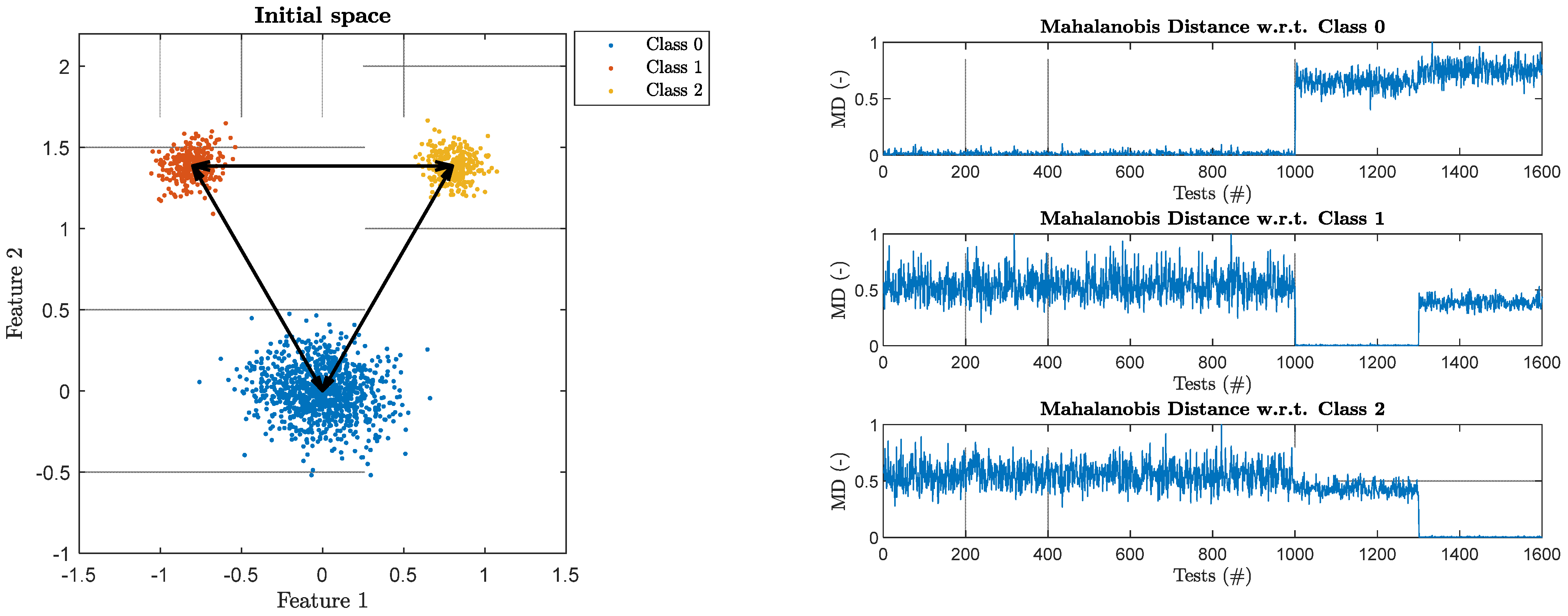
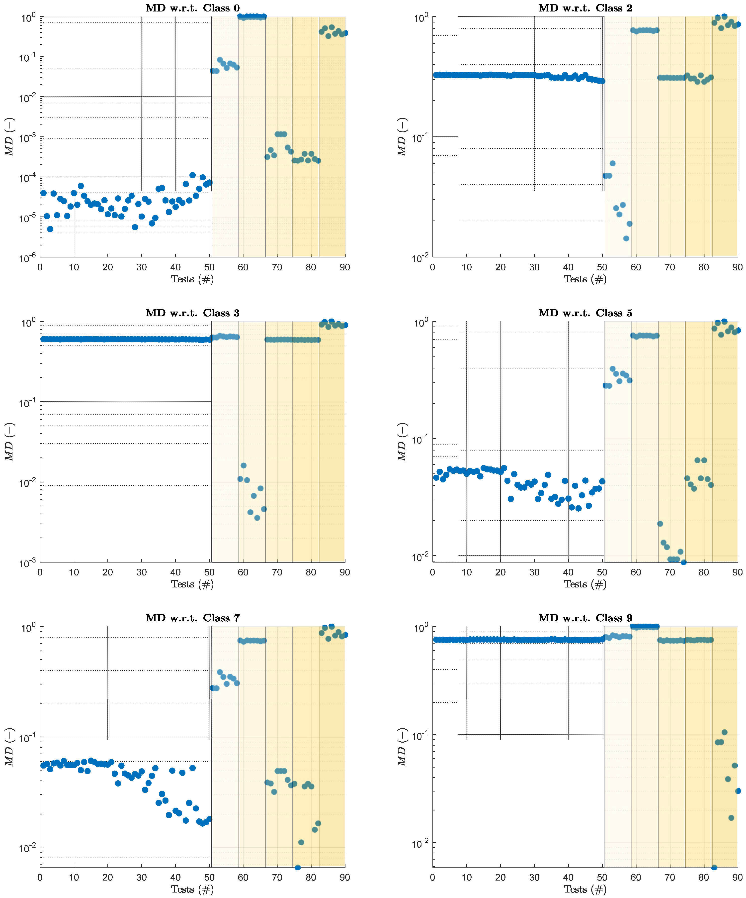
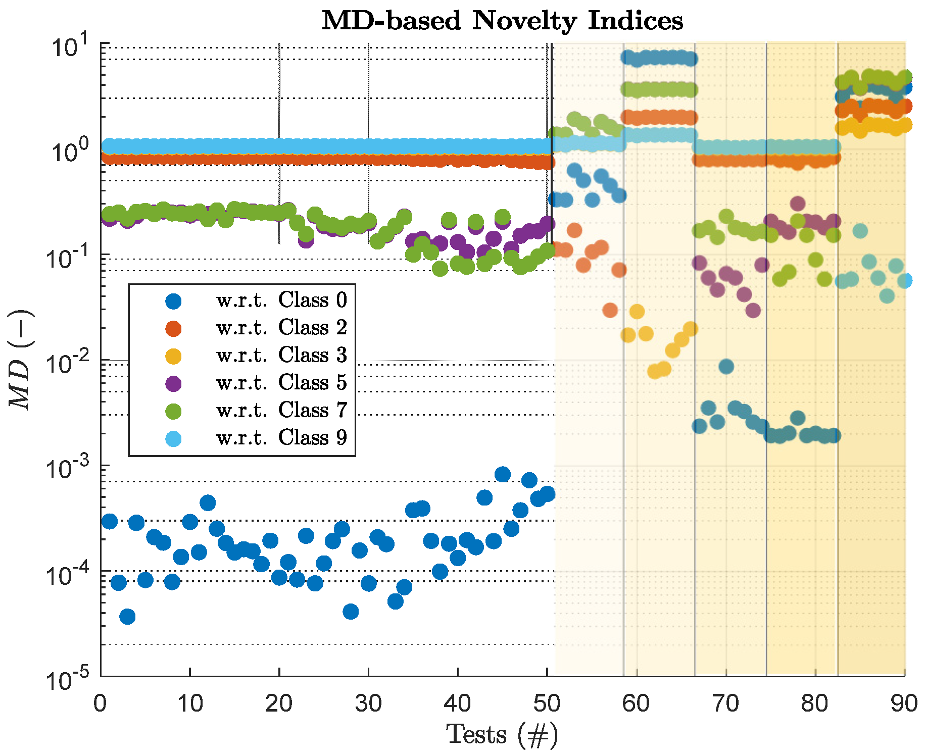
4.2. MD-Based Multi-Novelty Indices (MNI)

This second new method exploits ND principles using NIs based on the Mahalanobis distance. As mentioned in Section 3.2, MD is calculated by inverting the covariance matrix $\Sigma$ referred to the class of interest. Given the high number of features in the diagnostic field, an (almost) singular covariance matrix is likely to be obtained. For this reason, it is necessary to use a dimension reduction method and, in this case, the CCA is used as described in Section 4.1. After transforming the original data, a matrix in the optimized CCs variables is obtained (in this case, the matrix obtained has dimensions $m \times \left(k-1\right)$, where $m$ represents the tests performed and $k$ the number of classes of the dataset).

At this point, it would be easy to calculate a MD-based novelty index with reference to the healthy class data. The entire dataset is not used as a reference for the calculus of the covariance matrix since the multidimensional space would be deformed considering the variance of all data (belonging to both the healthy class and those with damage). In fact, the directions with maximum variance could highly vary due to the concentration of the clustered data. This would result in a deformation of the multidimensional space that is not consistent, consequently influencing the calculated MDs. While considering this aspect, the calculation of a single MD may not allow the correct recognition of all clusters, as the distance value does not consider the angular position of the data within the multidimensional space. This statement can be explained by Figure 5, in which three clusters are approximately equally spaced with respect to the MD in a 2D space. By calculating the MD of all points with respect to Class 0, Classes 1 and 2 are recognized but are not distinguishable from each other. The proposed method consists of the iterative calculation of the MD with respect to all the classes, thus obtaining $k$ NIs. Each $k$-th NIs set behaves as a one-class classification, failing to distinguish the other classes from each other. However, if each MD manages to solve a two-class problem, the use of $k$ MD would allow the unique recognition of $k$ clusters. Two groups of data would not be recognized only if they are indistinguishable (i.e., the point clouds lie in the same portion of the multidimensional space). This technique would allow the $n$ features of the original matrix to be reduced to $k$ features, in case the number of clusters $k$ is lower than $n$. Figure 6 shows an example of the new reduced space obtained thanks to the MD iteratively calculated with respect to each cluster. It can be noted that every cluster is well separated and distinguishable.

Although $k-1$ features are obtained before iteratively calculating the MDs thanks to CCA, these NIs exploit the covariance matrices inherent to each class and, therefore, take into account the distribution of the data. The resulting deformation of the space could potentially increase the distance between clusters. It consequently improves data recognition, as well as classification accuracy.

However, the dimensionality reduction carried out before the calculation of the MDs may not be sufficient as the $m_k$ number of performed tests per each class may not be high enough compared to the number of clusters $k$ present in the dataset. The covariance matrix would be singular again in such a case. The imbalance of data consists precisely in having a higher amount of data for one class than for the others, a fact that often occurs in the field of diagnostics of mechanical systems where the data recorded with the machinery in healthy conditions considerably exceed those obtained in anomalous conditions or with damage. As explained in [35], supervised learning performance is not systematically affected by class imbalance, but it would appear to depend mainly on the lack of sufficient data for minority classes and other factors such as class overlap. For this reason, before proceeding with the calculation of the MDs referring to each class, it is possible to apply some methods for balancing machine learning training data. A possible application consists of over-sampling methods (called ROS, which aim to balance the classes by inserting samples in the minority classes) possibly in combination with under-sampling (called RUS, which, on the contrary, aims to balance the classes by eliminating samples from the majority ones) [36]. The methods used in this work are among those most used in practice: Synthetic Minority Over-sampling Technique (Smote) [37] for the over-sampling and Tomek Links [38] for the under-sampling. The first method generates new examples of minority data by interpolating the different data of the same class. Even if class balancing is improved, further problems may arise. In fact, given that minority classes extend more in space, some examples of the majority and minority classes could become confused, thus worsening the recognition of clusters. For this reason, an under-sampling method, such as Tomek Links, could be applied later to eliminate noise or borderline points and to achieve a cleanup of the dataset. In addition to these methods, the creation of pseudo-points to balance the classes was also tested, simply by the duplication of the samples of the minority classes. This method does not add any information to the data. However, if the clusters are sufficiently separable, it could not aggravate the error and, at the same time, would allow the calculation of the covariance matrix for the minority classes.

Nevertheless, data balancing methods may not be sufficient to avoid a singular covariance matrix, especially in cases where the amount of data on the damage classes is very limited. Indeed, the number of tests considered to generate the covariance matrix must be large enough to derive the variance and covariance values of the new $k$-dimensional space. These values are used to transform the space and calculate the MDs. In this study, if a singular covariance matrix is obtained despite the application of data balancing methods, a simplification of the MD to the extreme case—reducing it to the Euclidean Distance (ED)—has been adopted.

5. Results and Discussion

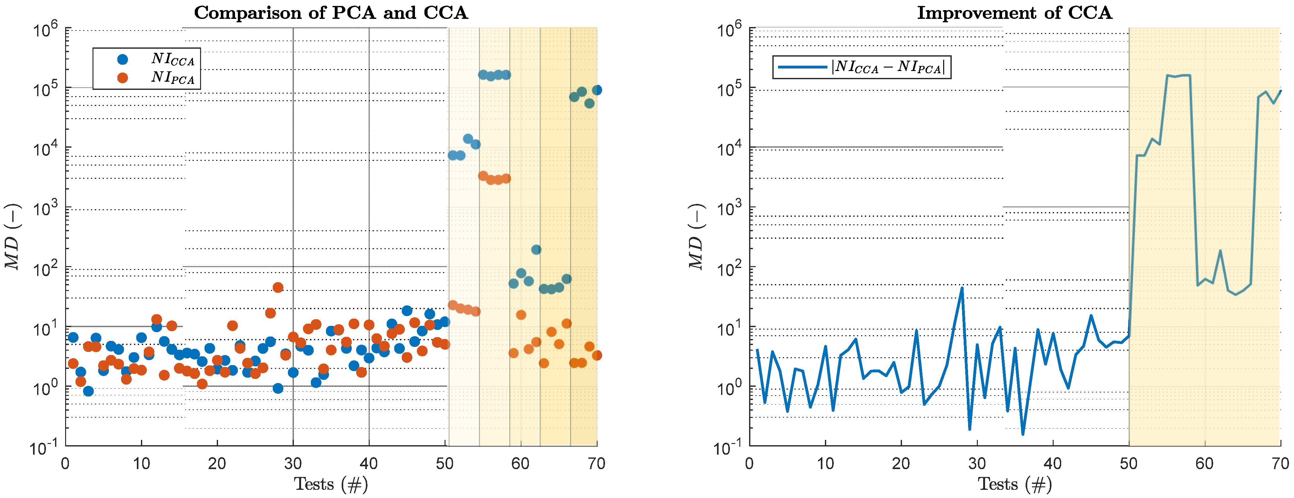
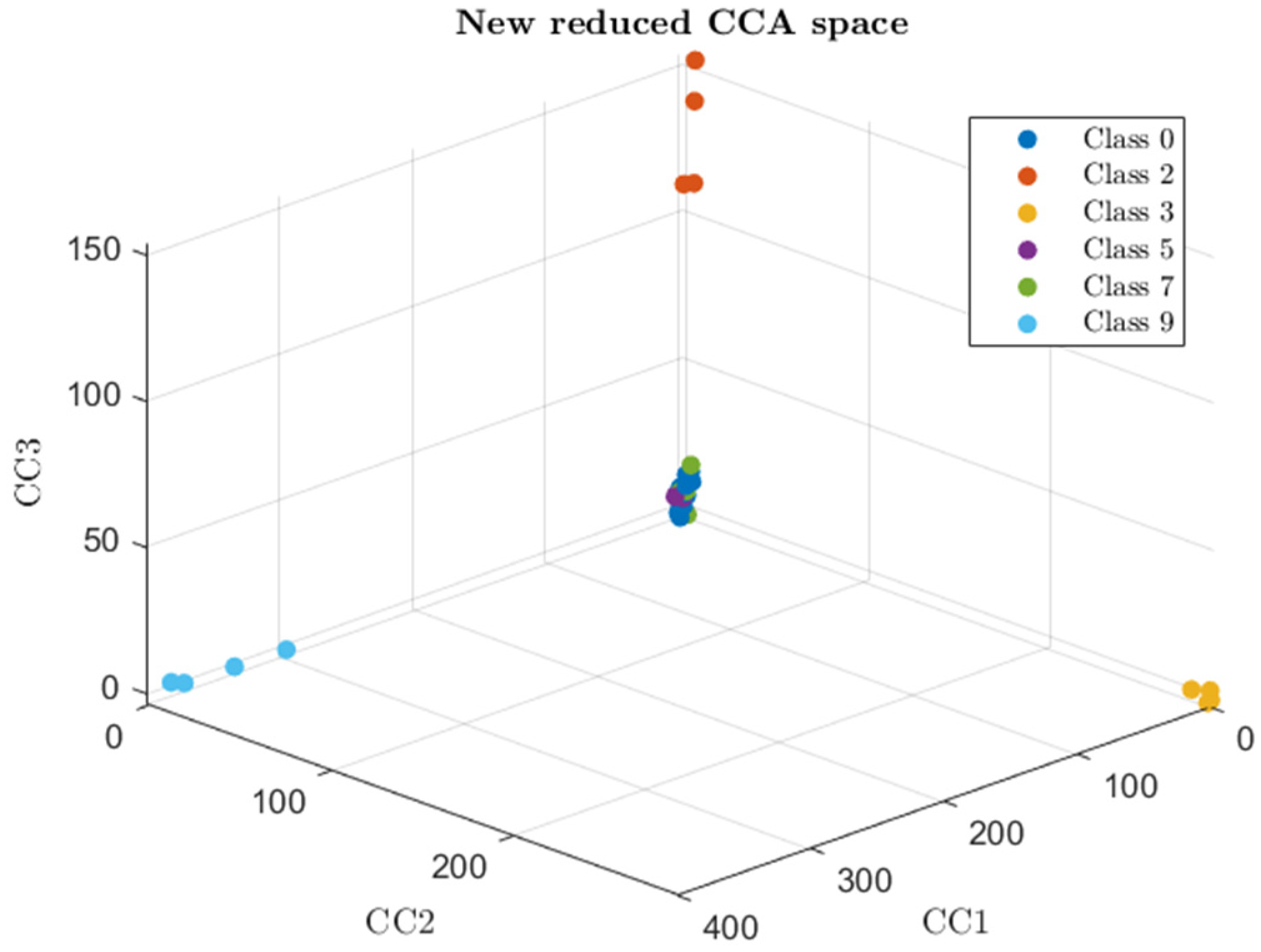
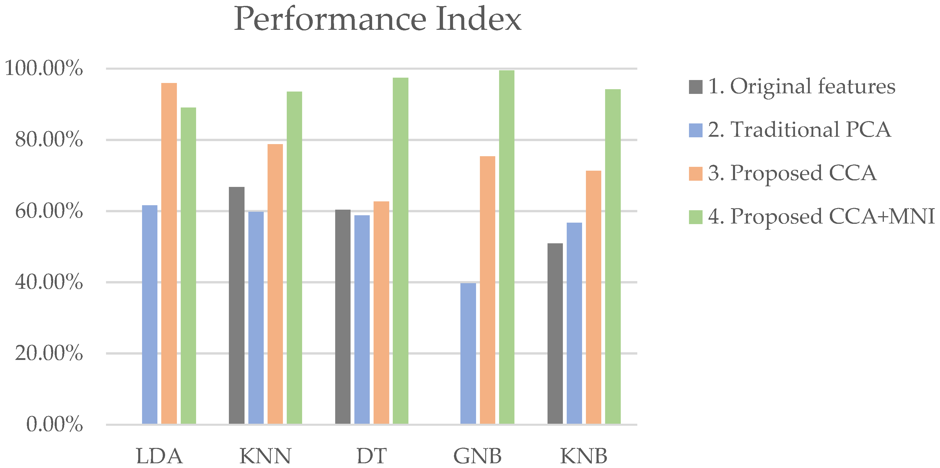
This section shows the results obtained on the PHME dataset [26] described in [22] with the application of the proposed DRM. After implementing each phase as described in Section 4 and obtaining the features in the new space with reduced dimensions, five of the main classification models were applied: Linear Discriminant Analysis (LDA) [39], k-Nearest Neighbor (kNN) with $k=2$ given the reduced amount of data for the minority classes [40], Decision Trees [41], Gaussian Naive Bayes and Kernel Naive Bayes [42]. The results were computed in terms of performance indices. It was decided to use those adopted in [22]—which are accuracy, missed alarms, false alarms, class errors rate, performance index, Frobenius norm and Area Under the Curve (AUC)—in order to effortlessly compare the two different methods.

The data used for this study were pre-processed with the same procedure adopted in [22]. The same holds true for the performance indices and the use of the Monte Carlo Cross-Validation method (MCCV) [43] to obtain the results convergence after $N=50$ iterations.

5.1. CCA Results

One goal of this research was to find a possible method to solve the clusters recognition problem related to PCA. In fact, in some particular cases dictated by the dispersion of data in the multivariate space, PCA can confuse clusters. In addition to this, PCA has a further complication due to the chosen number of features (i.e., the number of dimensions to be considered without excessively losing the information of the initial dataset). The proposed CCA aims at increasing the distance of the different clusters in the new space generated with reduced dimensions, thus allowing a better recognition of the test classes. Furthermore, the reduction in the number of dimensions is a function of the number of classes defined by the study of the specific machinery and the relative loss of information is theoretically about zero since all the initial features contribute to the new ones with different weights.

The goodness in clusters recognition and the improvement for this purpose compared to the traditional PCA can be measured initially by observing the MDs obtained with the ideal conditions class data (Class 0). Given that they only consider the distance with respect to the Class 0 center and not the angular position of the data, it is necessary to remember that the results obtained in terms of MD are mainly used to compare the improvement in terms of increasing the distance (and, therefore, recognition) of the data with respect to the reference class and not in a precise classification viewpoint. As can be seen in Figure 7, the clusters separation increased considerably with all the calculation alternatives. It is also possible to notice a better recognition of the classes themselves in addition to a greater spacing of the clustered data.

The comparison with respect to the MD cannot always be made with the entire initial $n$-dimensional dataset, as occurred with the dataset under analysis, since the covariance matrix is ill-conditioned when $m<n$, a status that often occurs when the considered features are in a large number. Indeed, this is a further simplification shared by both PCA and the proposed CCA. In particular, observing Figure 8, it is possible to notice how CCA kept the position of the reference Class 0 almost unvaried, while it increased the separation of the clusters representing the different damages with respect to PCA. This means a greater distance between clusters and, therefore, a potentially better recognition.

Moreover, it is possible to propose a comparison through the performance indices. The performance indices calculated using (1) the original dataset with $n$ features, (2) the first $k-1$ features obtained applying the traditional PCA and (3) the features calculated with the proposed CCA are reported in

Table 1. Performance indices obtained with the original dataset with $n$ features. It is worth noting that LDA and GNB were not applicable due to the high dimensionality of the dataset.

Index	LDA	KNN	Decision Tree	Gaussian N.B.	Kernel N.B.
Accuracy	-	81.5%	76.9%	-	71.4%
Missed Alarms	-	15.5%	6.5%	-	28.6%
False Alarms	-	1.5%	7.1%	-	0.1%
Class Errors	-	1.5%	9.6%	-	0.0%
P.I.	-	66.79%	60.39%	-	50.95%
Frobenius N.	-	2.35	2.04	-	3.16
AUC	-	0.99	1.00	-	1.00

,

Table 2. Performance indices obtained with the most relevant $k-1$ features calculated with traditional PCA.

Index	LDA	KNN	Decision Tree	Gaussian N.B.	Kernel N.B.
Accuracy	78.2%	76.7%	74.6%	60.0%	74.3%
Missed Alarms	14.1%	13.3%	16.2%	10.2%	13.6%
False Alarms	7.2%	6.5%	6.3%	22.8%	6.6%
Class Errors	0.5%	3.5%	3.0%	7.0%	5.5%
P.I.	62.0%	60.0%	56.8%	38.7%	56.7%
Frobenius N.	2.10	2.08	2.34	1.97	2.13
AUC	0.85	0.97	0.90	0.89	0.99

and

Table 3. Performance indices obtained using $k-1$ features calculated with the proposed CCA. The variations with respect to the reference PCA method (in Table 2) are shown in brackets. Please note that the percentage variations highlighted in green represent an improvement (increase in precision and decrease in errors), while those in red indicate a worsening in terms of performances.

Index	LDA		KNN		Decision Tree		Gaussian N.B.		Kernel N.B.
Accuracy	98.4%	(+20.3%)	94.2%	(+17.5%)	80.9%	(+6.3%)	89.4%	(+29.4%)	86.6%	(+12.3%)
Missed Alarms	1.3%	(−12.8%)	5.7%	(−7.6%)	5.0%	(−11.1%)	2.1%	(−8.1%)	6.6%	(−7.0%)
False Alarms	0.2%	(−7.0%)	0.1%	(−6.4%)	4.3%	(−2.0%)	7.1%	(−15.7%)	4.4%	(−2.2%)
Class Errors	0.0%	(−0.5%)	0.0%	(−3.5%)	9.8%	(+6.8%)	1.4%	(−5.5%)	2.4%	(−3.1%)
P.I.	96.9%	(+34.9%)	88.7%	(+28.7%)	66.3%	(+9.5%)	80.2%	(+41.5%)	75.4%	(+18.7%)
Frobenius N.	0.33	(−1.8)	1.12	(−1.0)	1.91	(−0.4)	0.59	(−1.4)	1.38	(−0.8)
AUC	1.00	(+0.2)	1.00	(0.0)	0.97	(+0.1)	0.99	(+0.1)	0.99	(0.0)

. The performance indices obtained by the PCA were considered as the reference to compare the results of the proposed technique. Given that the proposed method reduced the number of features to $k-1$, the first and most relevant $k-1$ features processed through PCA were considered in such a way as to make the comparison homogeneous and consistent.

According to the results in Table 1, Table 2 and Table 3, it is possible to state that the proposed CCA greatly improved data classification while decreasing data dimensionality. It is also possible to notice how, compared to the traditional PCA, a high degree of information deriving from the initial features was maintained. Furthermore, the number of selected features was chosen automatically based on the classes contained in the dataset, eliminating potential issues or errors arising in the standard PCA. For these reasons, CCA could be used as a selector of features in some particular cases in which the PCA is not able to assign (or does not perform optimally the assignment of) the data to the different labels.

However, as previously mentioned, this method requires the labels referring to a training dataset to generate the roto-translation matrix $\mathit{E}$ for the desired transformation. Hence, unlike traditional PCA, this cannot be regarded as an unsupervised learning method.

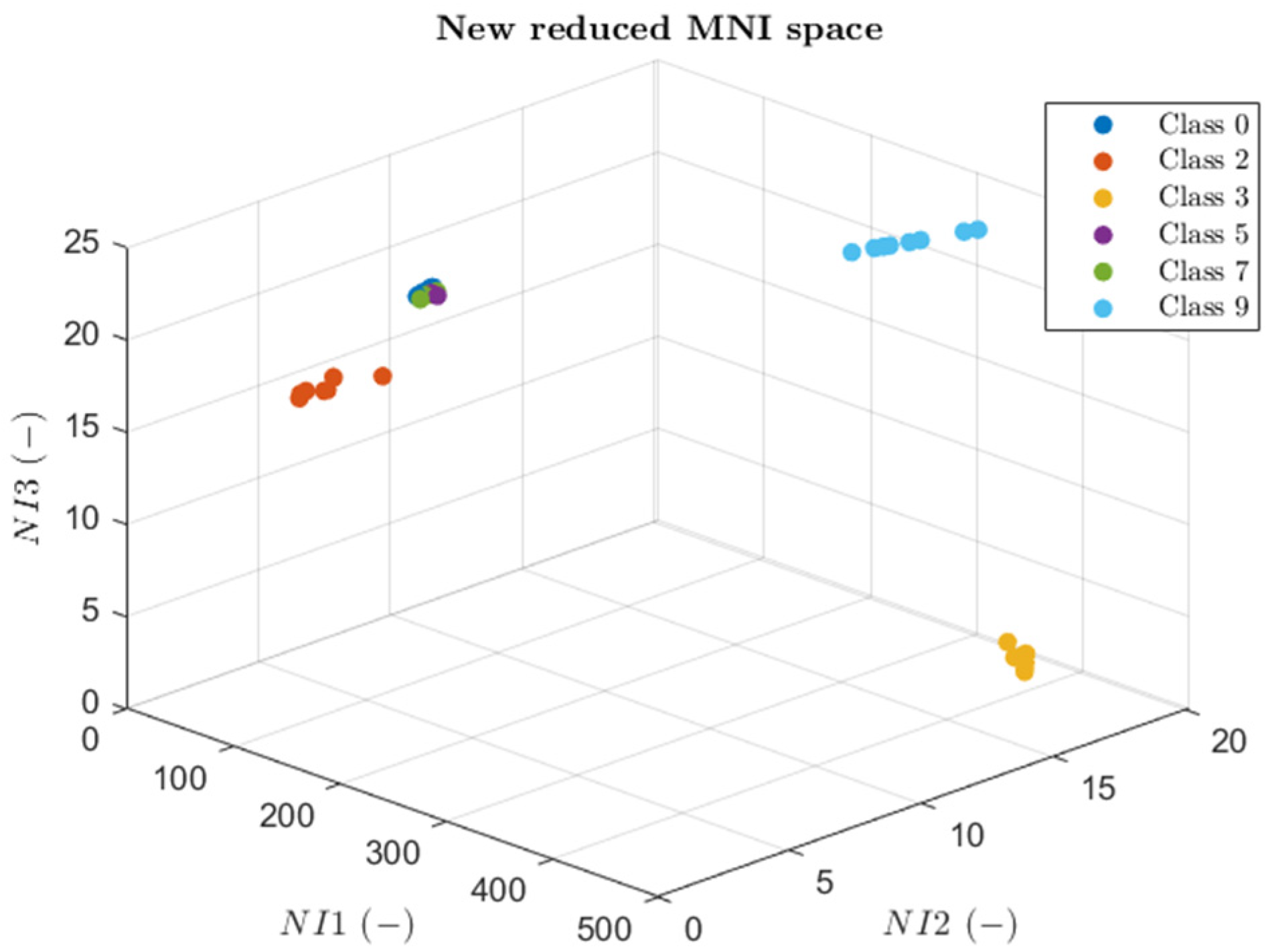
5.2. CCA+MNI Results

Since it is not possible to compute MNIs without initially reducing the original features space, the results of implementing the combination of the proposed techniques (CCA+MNI) are shown in this section. The performance indices obtained using only the proposed method highlight how the solely computation of MNIs affected the classification.

Just to recap, this second phase of the proposed method aims at reducing the dimensionality of the dataset by exploiting NIs based on MD. Conceptually, the proposed method resembled Gaussian Mixture Models (GMM), probabilistic models that describe points through the composition of a finite number of parameterized Gaussians. In fact, in the particular case in which the probability of a given $x$ belonging to a Class $k$ $P(x|k)$ with the covariance matrices ${\Sigma }_k$ and the probabilities $P\left(k\right)$ are equal for all classes, then the so-called Bayes’ maximum-a-posteriori (MAP) rule for classification corresponds to the Mahalanobis distance between the generic point $x$ and the mean value of the reference class [44]. MD can also be considered as a particular case of the Gaussian mixture distance having a unique combination of Gaussians. Although these two methods are conceptually similar, they do not necessarily perform in the same way. When the Gaussian Mixture distance is defined as a distance function calculated using a GMM, it is shown in [45] how the latter gave better results than MD with some datasets in terms of precision for data clustering tasks. However, Li et al. compared the Gaussian mixture distance with a single MD calculated by considering the covariance matrix of the entire dataset (and not of a single class). With the proposed method based on multi-MD, on the other hand, we wanted to improve the classification accuracy and reduce the dimensionality in terms of the number of features at the same time. In addition to this, the iterative calculation of the MDs uses the covariances related to each class $k$ and, unlike the GMMs, it is not necessary to use and optimize the parameters connected to the distributions and to the combination of the Gaussians. For this reason, the calculation of MD-based NIs highly simplifies the extraction of features as the creation of a Gaussian mixture model is complex due to the evaluation and optimization of the parameters.

The iterated calculation of MDs with respect to each class allows the problem of the directionality of the MD with consequent better recognition of the clusters to be eliminated. Figure 9 shows the tests with respect to the first three MDs (i.e., calculated with respect to Class 0, 2 and 3) and it is possible to observe a good separation of these classes. As can be seen from Figure 10, while with the use of a single MD it was possible to separate some classes from the healthy one (without, however, distinguishing them perfectly from each other), the simultaneous use of $k$ distances allowed not only better recognition conditions but also the distinction of all types of damage. The classification results achieved using $k-1$ NIs as input are shown in

Table 4. Performance indices obtained applying the proposed CRM entirely (CCA+MNI). SMOTE and Tomek Links methods were considered in the analysis for the data balancing. The variations with respect to the solely CCA pre-processing (in Table 3) are shown in brackets. Please note that the percentage variations highlighted in green represent an improvement (increase in precision and decrease in errors), while those in red indicate a worsening in terms of performances.

Index	LDA		KNN		Decision Tree		Gaussian N.B.		Kernel N.B.
Accuracy	97.6%	(−0.8%)	97.3%	(+3.1%)	98.2%	(+17.3%)	98.3%	(+8.9%)	97.8%	(+11.2%)
Missed Alarms	1.1%	(−0.2%)	2.4%	(−3.3%)	0.0%	(−5.0%)	0.0%	(−2.1%)	0.6%	(−5.9%)
False Alarms	1.3%	(+1.0%)	0.3%	(+0.2%)	0.0%	(−4.3%)	1.2%	(−5.8%)	0.0%	(−4.4%)
Class Errors	0.0%	(0.0%)	0.0%	(0.0%)	1.8%	(−8.0%)	0.5%	(−0.9%)	1.6%	(−0.9%)
P.I.	95.3%	(−1.6%)	94.7%	(+6.0%)	96.4%	(+30.1%)	96.6%	(+16.4%)	95.6%	(+20.2%)
Frobenius N.	0.18	(−0.2)	0.38	(−0.7)	0.27	(−1.6)	0.10	(−0.5)	0.29	(−1.1)
AUC	1.00	(0.0)	1.00	(0.0)	1.00	(0.0)	1.00	(0.0)	1.00	(0.0)

. Please remember that the Mahalanobis distances were calculated after the pre-processing through CCA, as described in the previous subsection, and applying both SMOTE and Tomek Links methods for balancing the data.

By comparing the obtained results in terms of performance indices (as shown in Figure 11), it is possible to observe how the proposed CRM—both CCA and the CCA+MNI combination—allowed the dimensionality of the dataset to be reduced by improving the classification and recognition of classes. It is worth noting that the combination of the proposed techniques always improved the classification performance with the only LDA exception. This could be explained by the fact that LDA—being a linear classifier—is able to better distinguish the clusters through the features produced by CCA (linear method) rather than through the MNIs (obtained through a nonlinear method). In addition to increasing accuracy and reducing false and missed alarms, the described method also allows errors in class recognition to be reduced. This means that it is possible to trace the type of damage present on the machinery and act in a specific way (prescriptive maintenance), as well as allowing good predictive maintenance.

6. Conclusions

This study concentrated on the problem of data dimensionality with a particular focus on applications in the field of mechanical machinery diagnostics. Although there are still numerous analyses such as PCA—one of the most widely used multifunctional multivariate statistical analyses—they do not always allow data patterns to be distinguished in all verifiable situations. For this reason, a novel DRM (consisting of the combination of two different techniques) was presented. This allowed datasets with particular characteristics to be pre-processed: high dimensionality in terms of number of features and data grouped in clusters. If these assumptions are valid, the proposed method can be applied to any high-dimensional clustered dataset without any limit to the application field. However, future developments could consider a numerical verification using different datasets. It was further demonstrated through an application example that the proposed model also allows work with datasets with insufficient information about the abnormal conditions, since the dataset could generally constitute a limitation of the data-driven models. In fact, data-driven approaches often require a large amount of labelled data for (semi-)supervised learning and it is not always easy to find a sufficient quantity of data, especially for damaged conditions

The first phase of the proposed method—named Clusters Component Analysis (CCA)—is based on the same principle of PCA, but allows better clusters recognition, as observed by the performance indices obtained for different classifiers. Firstly, CCA allows the dataset to be simplified in terms of dimensionality reduction. In detail, the number of selected features is automatically defined by the number of classes considered in the dataset. Furthermore, this procedure also minimizes the loss of information considering the weighted contribution of all the initial features. However, unlike the traditional PCA, this method requires each acquisition to be associated with a label. For this reason, CCA can be considered as a (semi-)supervised learning method.

The second phase of the proposed method exploits several novelty indices (hence the name Multi-Novelty Indices) based on the Mahalanobis distance to improve the classification. Indeed, the calculation of a single MD may not always allow the correct recognition of all the clusters since, being a distance, it cannot consider the angular position of the data within the multidimensional space.

Finally, it should be noted that several models existing in the literature (e.g., developed in [22]) are parametric, unlike the proposed one. Indeed, while the choice of parameters for the routine of a Genetic Algorithm (GA) could be more complex and expensive, CCA and MNI calculus are more immediate and straightforward to apply as they are not parametric models. Although the results proposed in the previous method [22] were satisfactory, the present CCA and MNI methods provided an additional improvement in accuracy and performance index equal to 5.0% and 9.4%, respectively, on average, using the same dataset and pre-processing.

In general, the proposed DRM showed very good performance indices for the different classifiers (accuracy equal to 98% on average) and improvements compared to other techniques. The dimensionality of the reduced space depends on the number of fault classes present in the dataset. A further common advantage (and strictly linked to the reduction of dimensionality) concerns memory occupation for data acquisition, which can be considerably reduced. All the results shown are inherent to applications in the field of diagnostics of mechanical systems. Indeed, a pre-established class (inherent to the ideal conditions of a machine) has always been used as a reference for models. This does not mean that different classes cannot be used alternatively, but this investigation is left to future works.

References

1. Worden, K.; Dulieu-Barton, J.M. An Overview of Intelligent Fault Detection in Systems and Structures. Struct. Health Monit. 2004, 3, 85–98. [Google Scholar] [CrossRef]
2. Köppen, M. The Curse of Dimensionality. In Proceedings of the 5th Online World Conference on Soft Computing in Industrial Applications (WSC5), On the Internet (World-Wide-Web), 4–18 September 2000; Volume 1, pp. 4–8. [Google Scholar]
3. Huang, X.; Wu, L.; Ye, Y. A Review on Dimensionality Reduction Techniques. Int. J. Pattern Recognit. Artif. Intell. 2019, 33, 1950017. [Google Scholar] [CrossRef]
4. Cunningham, J.P.; Ghahramani, Z. Linear Dimensionality Reduction: Survey, Insights, and Generalizations. J. Mach. Learn. Res. 2015, 16, 2859–2900. [Google Scholar]
5. Ting, D.; Jordan, M.I. On Nonlinear Dimensionality Reduction, Linear Smoothing and Autoencoding. arXiv 2018, arXiv:1803.02432. [Google Scholar]
6. Zubova, J.; Kurasova, O.; Liutvinavičius, M. Dimensionality Reduction Methods: The Comparison Of Speed And Accuracy. Inf. Technol. Control 2018, 47, 151–160. [Google Scholar] [CrossRef]
7. Nguyen, L.H.; Holmes, S. Ten Quick Tips for Effective Dimensionality Reduction. PLoS Comput. Biol. 2019, 15, e1006907. [Google Scholar] [CrossRef] [Green Version]
8. Sophian, A.; Tian, G.Y.; Taylor, D.; Rudlin, J. A Feature Extraction Technique Based on Principal Component Analysis for Pulsed Eddy Current NDT. NDT Int. 2003, 36, 37–41. [Google Scholar] [CrossRef]
9. Wold, S.; Geladi, P.; Esbensen, K.; Öhman, J. Multi-Way Principal Components-and PLS-Analysis. J. Chemom. 1987, 1, 41–56. [Google Scholar] [CrossRef]
10. Fukumizu, K.; Bach, F.R.; Jordan, M.I. Dimensionality Reduction for Supervised Learning with Reproducing Kernel Hilbert Spaces. J. Mach. Learn. Res. 2004, 5, 73–99. [Google Scholar]
11. Schölkopf, B.; Smola, A.; Müller, K.-R. Nonlinear Component Analysis as a Kernel Eigenvalue Problem. Neural Comput. 1998, 10, 1299–1319. [Google Scholar] [CrossRef] [Green Version]
12. Chandrashekar, G.; Sahin, F. A Survey on Feature Selection Methods. Comput. Electr. Eng. 2014, 40, 16–28. [Google Scholar] [CrossRef]
13. Jardine, A.K.S.; Lin, D.; Banjevic, D. A Review on Machinery Diagnostics and Prognostics Implementing Condition-Based Maintenance. Mech. Syst. Signal Process. 2006, 20, 1483–1510. [Google Scholar] [CrossRef]
14. Daga, A.P.; Garibaldi, L.; Fasana, A.; Marchesiello, S. ANOVA and Other Statistical Tools for Bearing Damage Detection. In Proceedings of the International Conference Surveillance, Fez, Morocco, 23 May 2017; pp. 22–24. [Google Scholar]
15. Daga, A.P.; Garibaldi, L. Machine Vibration Monitoring for Diagnostics through Hypothesis Testing. Information 2019, 10, 204. [Google Scholar] [CrossRef]
16. Castellani, F.; Garibaldi, L.; Daga, A.P.; Astolfi, D.; Natili, F. Diagnosis of Faulty Wind Turbine Bearings Using Tower Vibration Measurements. Energies 2020, 13, 1474. [Google Scholar] [CrossRef] [Green Version]
17. Daga, A.P.; Garibaldi, L.; He, C.; Antoni, J. Key-Phase-Free Blade Tip-Timing for Nonstationary Test Conditions: An Improved Algorithm for the Vibration Monitoring of a SAFRAN Turbomachine from the Surveillance 9 International Conference Contest. Machines 2021, 9, 235. [Google Scholar] [CrossRef]
18. Worden, K. Structural Fault Detection Using a Novelty Measure. J. Sound Vib. 1997, 201, 85–101. [Google Scholar] [CrossRef]
19. Daga, A.P.; Fasana, A.; Garibaldi, L.; Marchesiello, S. On the Use of PCA for Diagnostics via Novelty Detection: Interpretation, Practical Application Notes and Recommendation for Use. In Proceedings of the PHM Society European Conference, Turin, Italy, 1 July 2020; Volume 5, p. 13. [Google Scholar]
20. Pimentel, M.A.; Clifton, D.A.; Clifton, L.; Tarassenko, L. A Review of Novelty Detection. Signal Process. 2014, 99, 215–249. [Google Scholar] [CrossRef]
21. Japkowicz, N.; Myers, C.; Gluck, M. A Novelty Detection Approach to Classification. In Proceedings of the Fourteenth Joint Conference on Artificial Intelligence, Montreal, QC, Canada, 20–25 August 1995; pp. 518–523. [Google Scholar]
22. Viale, L.; Daga, A.P.; Fasana, A.; Garibaldi, L. From Novelty Detection to a Genetic Algorithm Optimized Classification for the Diagnosis of a SCADA-Equipped Complex Machine. Machines 2022, 10, 270. [Google Scholar] [CrossRef]
23. Ebeling, B.; Vargas, C.; Hubo, S. Combined Cluster Analysis and Principal Component Analysis to Reduce Data Complexity for Exhaust Air Purification. Open Food Sci. J. 2013, 7, 8–22. [Google Scholar] [CrossRef] [Green Version]
24. Ding, C.; He, X.; Zha, H.; Simon, H.D. Adaptive Dimension Reduction for Clustering High Dimensional Data. In Proceedings of the 2002 IEEE International Conference on Data Mining, Maebashi City, Japan, 9–12 December 2002; pp. 147–154. [Google Scholar]
25. Data Challenge-PHME21. Available online: https://github.com/PHME-Datachallenge/Data-Challenge-2021 (accessed on 22 March 2022).
26. Biggio, L.; Russi, M.; Bigdeli, S.; Kastanis, I.; Giordano, D.; Gagar, D. PHME Data Challenge. In Proceedings of the European Conference of the Prognostics and Health Management Society, Virtual Event, 28 June–2 July 2021. [Google Scholar]
27. Sammut, C.; Webb, G.I. Encyclopedia of Machine Learning; Springer Science & Business Media: Berlin/Heidelberg, Germany, 2011. [Google Scholar]
28. MacKay, D.J.; Mac Kay, D.J. Information Theory, Inference and Learning Algorithms; Cambridge University Press: Cambridge, UK, 2003. [Google Scholar]
29. Natili, F.; Daga, A.P.; Castellani, F.; Garibaldi, L. Multi-Scale Wind Turbine Bearings Supervision Techniques Using Industrial SCADA and Vibration Data. Appl. Sci. 2021, 11, 6785. [Google Scholar] [CrossRef]
30. Abdi, H.; Williams, L.J. Principal Component Analysis. Wiley Interdiscip. Rev. Comput. Stat. 2010, 2, 433–459. [Google Scholar] [CrossRef]
31. Lever, J.; Krzywinski, M.; Altman, N. Points of Significance: Principal Component Analysis. Nat. Methods 2017, 14, 641–643. [Google Scholar] [CrossRef] [Green Version]
32. De Maesschalck, R.; Jouan-Rimbaud, D.; Massart, D.L. The Mahalanobis Distance. Chemom. Intell. Lab. Syst. 2000, 50, 1–18. [Google Scholar] [CrossRef]
33. Pearson, R.K. Outliers in Process Modeling and Identification. IEEE Trans. Control. Syst. Technol. 2002, 10, 55–63. [Google Scholar] [CrossRef] [PubMed]
34. Schmidt, E. Zur Theorie Der Linearen Und Nichtlinearen Integralgleichungen. In Integralgleichungen und Gleichungen mit Unendlich Vielen Unbekannten; Springer: Berlin/Heidelberg, Germany, 1989; pp. 190–233. [Google Scholar]
35. Batista, G.E.; Prati, R.C.; Monard, M.C. A Study of the Behavior of Several Methods for Balancing Machine Learning Training Data. ACM SIGKDD Explor. Newsl. 2004, 6, 20–29. [Google Scholar] [CrossRef]
36. Elhassan, T.; Aljurf, M. Classification of Imbalance Data Using Tomek Link (t-Link) Combined with Random under-Sampling (Rus) as a Data Reduction Method. Glob. J. Technol. Optim. S 2016, 1, 1–11. [Google Scholar] [CrossRef]
37. Chawla, N.V.; Bowyer, K.W.; Hall, L.O.; Kegelmeyer, W.P. SMOTE: Synthetic Minority over-Sampling Technique. J. Artif. Intell. Res. 2002, 16, 321–357. [Google Scholar] [CrossRef]
38. Tomek, I. Two Modifications of CNN. IEEE Trans. Syst. Man Cybern. 1976, SMC-6, 769–772. [Google Scholar]
39. Tharwat, A.; Gaber, T.; Ibrahim, A.; Hassanien, A.E. Linear Discriminant Analysis: A Detailed Tutorial. AI Commun. 2017, 30, 169–190. [Google Scholar] [CrossRef] [Green Version]
40. Kataria, A.; Singh, M.D. A Review of Data Classification Using K-Nearest Neighbour Algorithm. Int. J. Emerg. Technol. Adv. Eng. 2013, 3, 354–360. [Google Scholar]
41. Myles, A.J.; Feudale, R.N.; Liu, Y.; Woody, N.A.; Brown, S.D. An Introduction to Decision Tree Modeling. J. Chemom. 2004, 18, 275–285. [Google Scholar] [CrossRef]
42. Wickramasinghe, I.; Kalutarage, H. Naive Bayes: Applications, Variations and Vulnerabilities: A Review of Literature with Code Snippets for Implementation. Soft Comput. 2021, 25, 2277–2293. [Google Scholar] [CrossRef]
43. Xu, Q.-S.; Liang, Y.-Z. Monte Carlo Cross Validation. Chemom. Intell. Lab. Syst. 2001, 56, 1–11. [Google Scholar] [CrossRef]
44. Torra, V.; Narukawa, Y. On a Comparison between Mahalanobis Distance and Choquet Integral: The Choquet–Mahalanobis Operator. Inf. Sci. 2012, 190, 56–63. [Google Scholar] [CrossRef]
45. Li, X.Q.; King, I. Gaussian Mixture Distance for Information Retrieval. In Proceedings of the IJCNN’99. International Joint Conference on Neural Networks. Proceedings (Cat. No. 99CH36339), Washington, DC, USA, 10–16 July 1999; Volume 4, pp. 2544–2549. [Google Scholar]
Figure 1. Equipment: 4-axis SCARA-robot picking up electrical fuses with a vacuum gripper, from a feeder to a fuse-test-bench for a large-scale quality-control. Arrows represent the main phases involved in the quality-control process: (1) picking up, (2) thermal camera control, (3) sorting, (4), (5) transport and (6) storage.
Machines 11 00036 g001
Figure 2. Limitations of PCA: missing (a) nonlinear pattern, (b) nonorthogonal patterns and (c) obscured clusters. PC1 and PC2 are shown in blue and orange, respectively.
Machines 11 00036 g002
Figure 3. Flowchart summarizing the proposed and reference methods. Please note that CCA could also be applied independently.
Machines 11 00036 g003
Figure 4. Qualitative representation of a multivariate clustered dataset and of the v k vectors which connect the centers of Classes k clusters with the reference Class 0. The dash-dotted lines represent the PCA results on the whole dataset.
Machines 11 00036 g004
Figure 5. Two-dimensional exemplary representation of the multivariate initial space of three approximately equally spaced clusters (left). Representation and trend of the Mahalanobis distances of the same points (right). The graphs show the MDs calculated with respect to each cluster.
Machines 11 00036 g005
Figure 6. Representation of the new reduced space whose dimensions correspond to the MDs calculated iteratively. The clusters are well separated and distinguishable.
Machines 11 00036 g006
Figure 7. On the left, a comparison of the MDs calculated using a traditional PCA pre-processing and the proposed CCA pre-processing to improve the recognition of clusters. Vertical lines divide the different classes of damage. On the right, the improvement due to CCA in terms of higher separation of clusters in the new reduced space is shown. Please note that the vertical line distinguishes health and damaged classes to highlight how CCA kept the position of the reference Class 0 almost unvaried, while it increased the separation of the clusters representing the different damages.
Machines 11 00036 g007
Figure 8. Data arrangement with respect to three of the reduced dimensions by CCA (the reference class is the health one, outliers were removed and the vectors were orthogonalized).
Machines 11 00036 g008
Figure 9. Representation of the first 3 Mahalanobis distances (i.e., calculated with respect to groups 0, 2 and 3).
Machines 11 00036 g009
Figure 10. Trends of MNIs (mixture of Mahalanobis and Euclidean distances, depending on the singularity of Σ k matrix) calculated and standardized with respect to each class after a data balancing through SMOTE and T-Links.
Machines 11 00036 g010aMachines 11 00036 g010b
Figure 11. Comparison chart related to the performance index obtained using the original features, the reference DRM and the proposed one (showing partial result of each phase) as the type of classifier varies.
Machines 11 00036 g011