1. Introduction
In recent years, UAVs have been widely used in the military by virtue of their stealth and high maneuverability. The small and medium-sized UAVs are widely used on the battlefield to attack important enemy targets because of their small size and the ability to evade radar detection by flying at low or ultra-low altitudes [
1,
2,
3,
4]. In addition, under the original technology, UAVs were controlled by rear operators for all operations and did not achieve unmanned operation in the true sense. Further, with the advancement of artificial intelligence technology, UAV intelligent pilot technology has also been rapidly developed, and UAV autonomous control can be realized in many functions. However, in order to further enhance the UAV’s autonomous control capability, research on UAV path planning, real-time communication, and information processing needs to be strengthened. Among them, UAV autonomous path planning is a hot issue attracting current researchers’ attention [
5,
6,
7,
8].
The path planning problem can be described as finding an optimal path from the current point to the target point under certain constraints, and many algorithms have been used so far to solve UAV path planning problems in complex unknown environments. Nowadays, the common path planning algorithms are the A*algorithm, the artificial potential field algorithm, the genetic algorithm, and the reinforcement learning method [
9,
10]. In recent years, deep learning (DL) and reinforcement learning (RL) have achieved a lot of results in many fields. Deep learning (DL) has strong data fitting ability, and reinforcement learning (RL) can model the process reasonably and can be trained without labels [
11,
12,
13] combined the advantages of DL and RL to obtain deep reinforcement learning (DRL), which provides a solution to the problem of perception and decision-making for UAVs in complex environments [
14].
The DRL can effectively solve problems with both continuous and discrete spaces. Therefore, many researchers proposed using DRL to solve the path planning problem. Mnih, V., et al. proposed the deep Q-network (DQN) algorithm [
15] by combining Q-learning and deep learning to solve the problem of dimensional explosion triggered by high-dimensional inputs. The DQN algorithm has achieved greater results in discrete action and state spaces but cannot effectively solve the continuous state and action spaces. In addition, when the changes of states and actions are infinitely partitioned, the amount of data for states and actions will show exponential growth with the increase of degrees of freedom, which can significantly impede the training and ultimately result in the algorithm failing [
16]. Moreover, the discretized state and action space actually removes a large amount of important information, which will eventually lead to poor control accuracy, which will not meet the requirements for UAV control accuracy in air warfare. The actor-critic (AC) algorithm has the ability to handle the continuous action problem and is therefore widely used to solve problems in the continuous action space [
17].The network structure of the AC algorithm includes an actor network and a critic network, actor network is responsible for outputting the action, and the critic network evaluates the value of the action and uses a loss function to continuously update the network parameters to get the optimal action strategy [
18]. However, the effect of the AC algorithm relies heavily on the judgment of the value of the critic network, and the critic network converges slowly, which leads to the actor network. Lillicrap, T.P. et al. [
19] proposed the deep deterministic policy gradient (DDPG) algorithm. The DDPG builds on the DQN algorithm’s principles and combines the Actor-Critic algorithm’s framework with several enhancements over the original AC algorithm to more effectively tackle the path planning problem in static environments. However, when applying the DDPG algorithm to solve path planning problems in dynamic environments, there is the problem of overvaluation of the value network, which leads to slow model convergence and a low training success rate. Scott Fujimoto [
20] et al. improved on the deep deterministic policy gradient (DDPG) algorithm to obtain the twin delayed deep deterministic policy gradient (TD3) algorithm, which is the TD3 algorithm that incorporates the idea of the double DQN algorithm [
21] into the DDPG algorithm, which effectively solves the problem of difficult algorithm convergence in a dynamic environment.
In this paper, a state detection method is proposed and combined with a dual-delay deep deterministic policy gradient (TD3) to form the SD-TD3 algorithm, which can solve the global path planning problem of a UAV in a dynamic battlefield environment and also identify and avoid obstacles. The main contributions of this paper are as follows:
(1) After combining the battlefield environment information, the information interaction mode between UAV and the battlefield environment is analyzed, a simulation environment close to the real battlefield environment is built, and the motion model of UAV autonomous path planning is constructed.
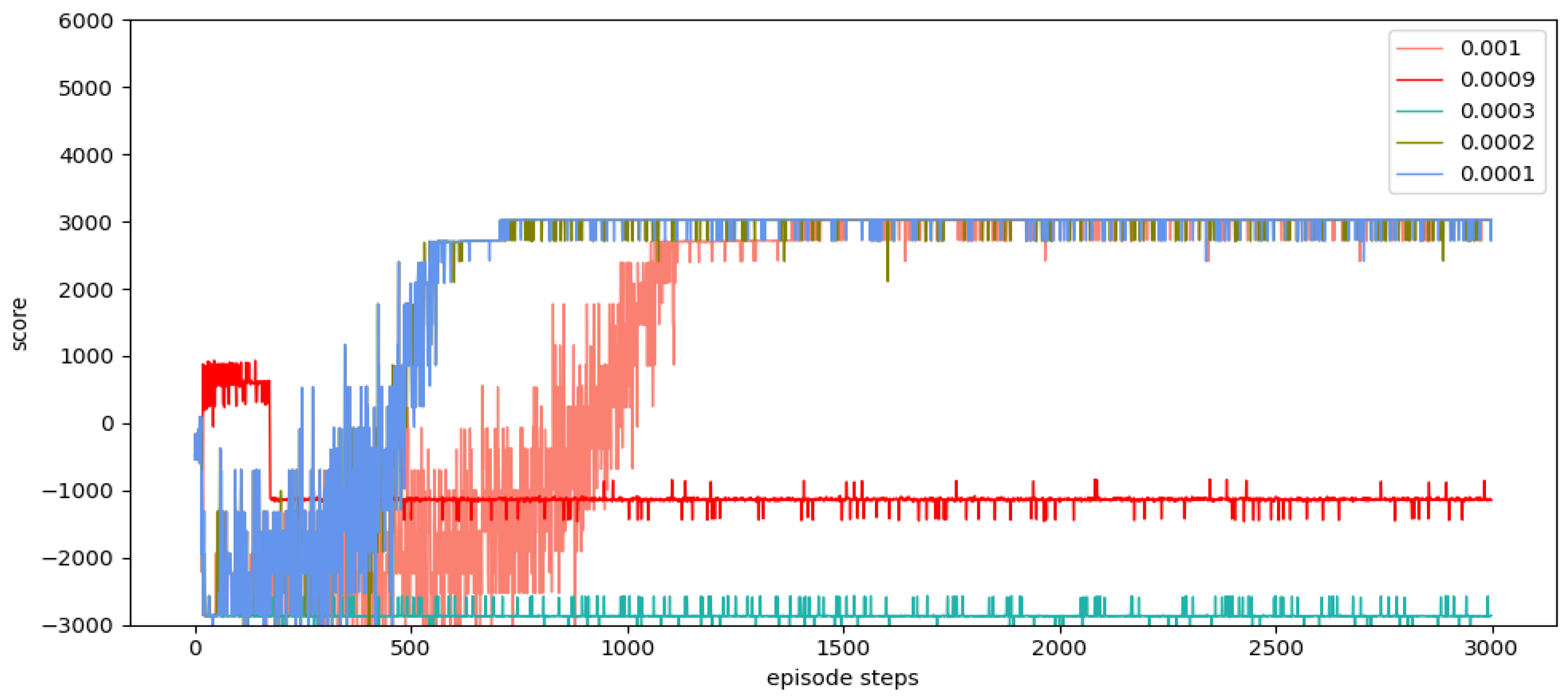
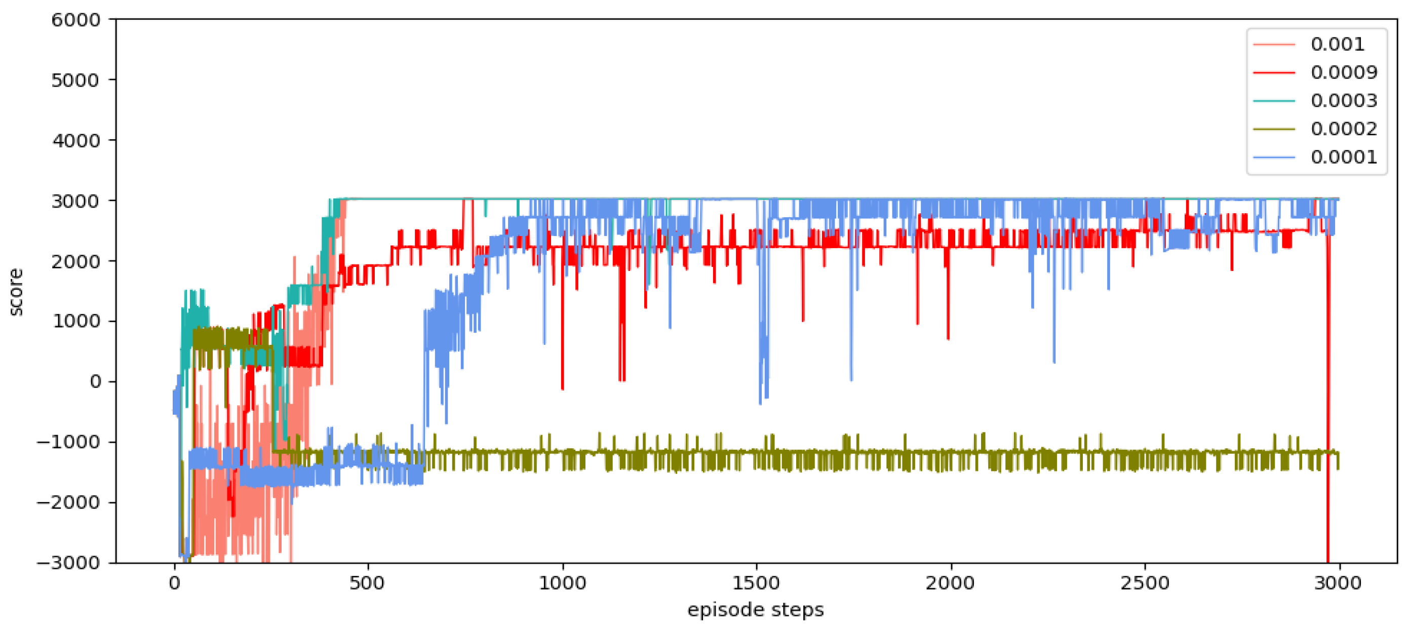
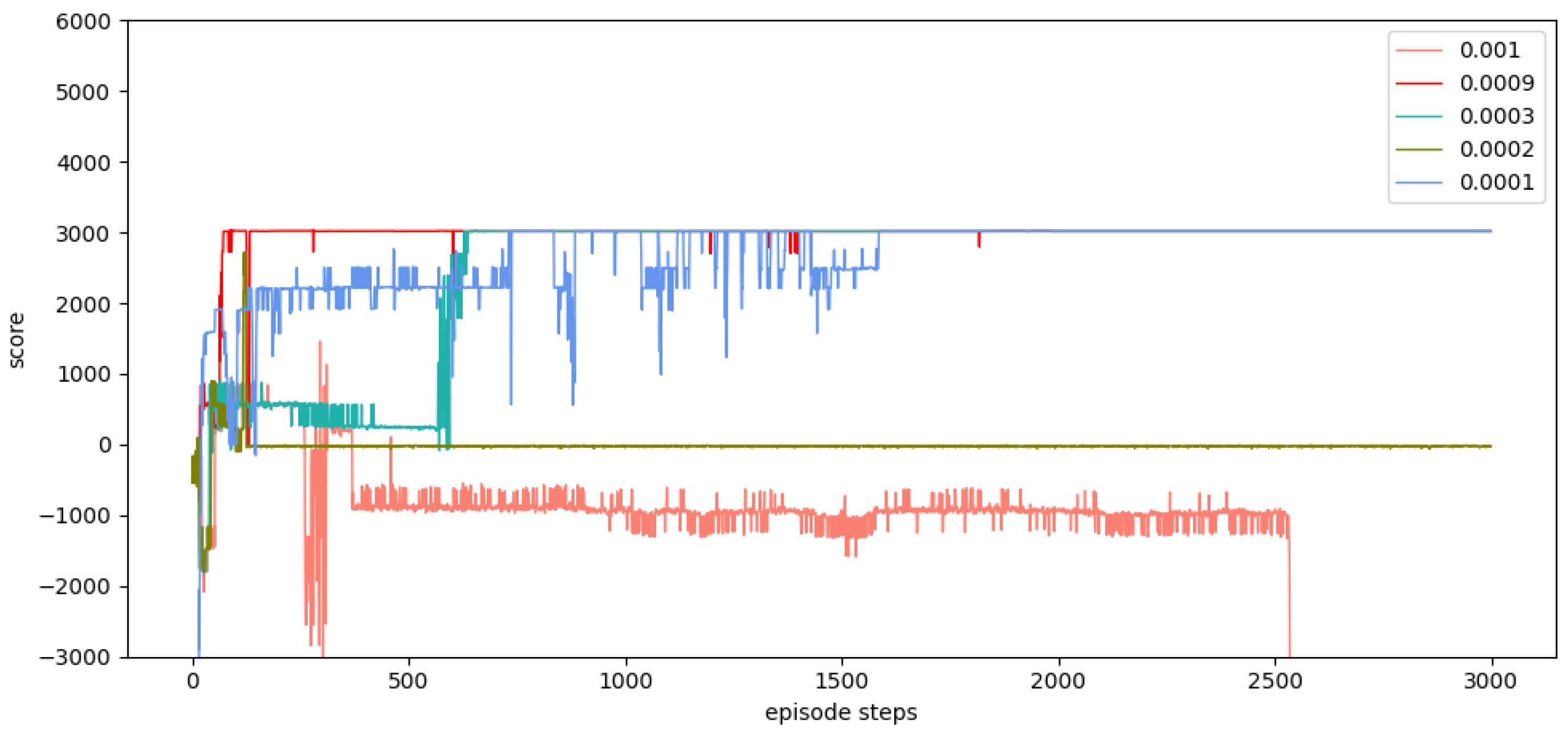
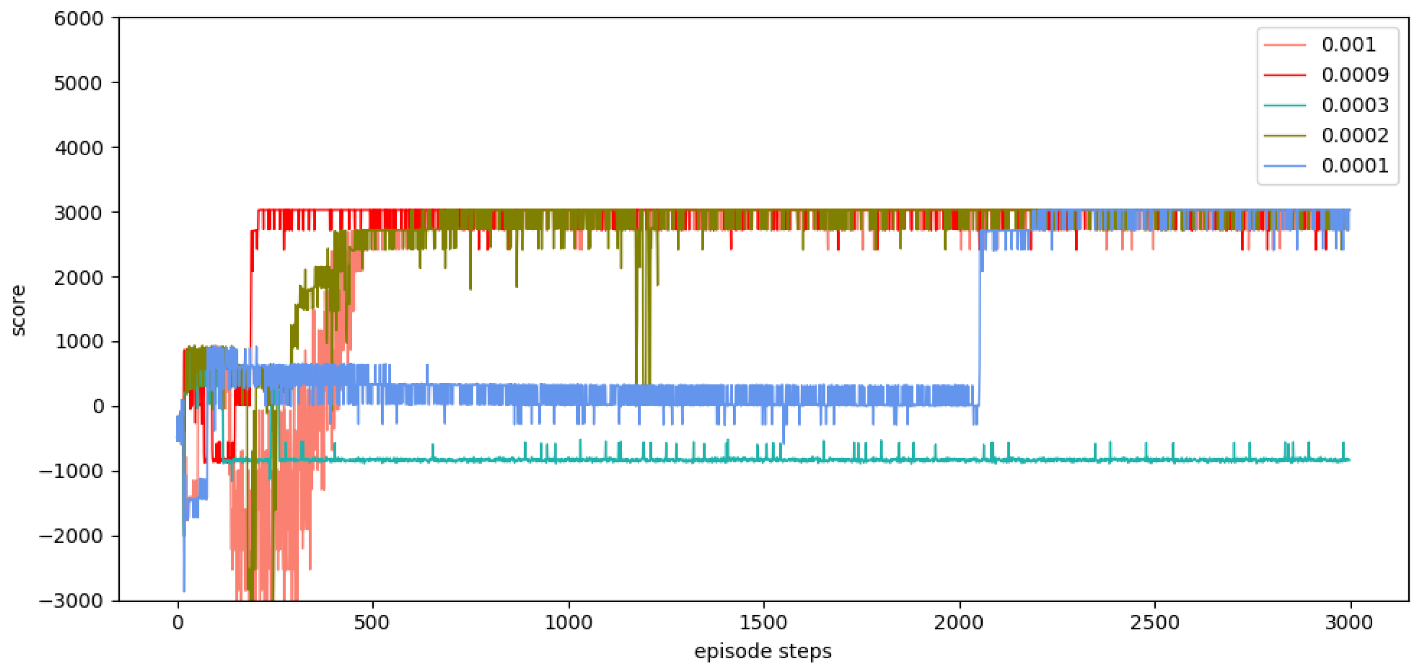
(2) The network structure and parameters most suitable for the SD-TD3 algorithm model are determined through multiple experiments. A heuristic dynamic reward function and a noise discount factor are also designed to improve the reward sparsity problem and effectively improve the learning efficiency of the algorithm.
(3) A state detection method is proposed that divides and compresses the environment state space in the direction of the UAV and encodes the space state by a binary number, so as to solve the problem of data explosion in the continuous state space of the reinforcement learning algorithm.
(4) The simulation experiments are carried out to verify the performance of the SD-TD3 algorithm, and the simulation experiments are based on the model of a UAV performing a low airspace raid mission. The results show that the SD-TD3 algorithm can help the UAV avoid radar detection areas, mountains, and random dynamic obstacles in low-altitude environments so that it can safely and quickly complete the low-altitude raid mission.
(5) By analyzing the experimental results, it can be concluded that the SD-TD3 algorithm has a faster training convergence speed and a better ability to avoid dynamic obstacles than the TD3 algorithm, and it is verified that the SD-TD3 algorithm can further refine the environmental state information to improve the reliability of the algorithm model, so that the trained algorithm model has a higher success rate in practical applications.
The rest of the paper is structured as follows, with related work presented in Part II. The third part models and analyzes the battlefield environment. Part IV describes the state detection scheme, the specific structure of the SD-TD3 algorithm, and the setting of the heuristic reward function, and Part V verifies the performance of the SD-TD3 algorithm through a simulation environment and analyzes the experimental results. The conclusion is given in the sixth part.
2. Related Work
In recent years, a lot of research on autonomous UAV path planning has been carried out at home and abroad, which can be divided into four categories of algorithms according to their nature: graph search algorithms, linear programming algorithms, intelligent optimization algorithms, and reinforcement learning algorithms.
The graph search algorithm mainly contains the Dijkstra algorithm, the RRT algorithm, the A* algorithm, the D* algorithm, etc. The most classical Dijkstra algorithm shows higher search efficiency than depth-first search or breadth-first search in the problem of finding the shortest path. However, the execution efficiency of the Dijkstra algorithm gradually decreases as the map increases. Ferguson, D. et al. [
22] optimized Dijkstra and proposed the A* and D* algorithms. Zhan et al. [
23] proposed an UAV path planning based on the improved A* algorithm for the path planning problem of low altitude UAVs in a 3D battlefield environment that satisfies UAV performance constraints such as safe lift and turn radii. Saranya, C. et al. [
24] proposed an improved D* algorithm for the path planning problem in complex environments, which introduced slope into the reward function. The simulations and experiments proved the effectiveness of the method, which can be used to guarantee the flight safety of UAVs in complex environments. Li, Z. et al. [
25] applied the RRT algorithm to the unmanned ship path planning problem, and an improved fast extended random tree algorithm (Bi-RRT) is proposed. The simulation results show that the optimized RRT algorithm can shorten the planning time and reduce the number of iterations, which has better feasibility and effectiveness.
The linear programming algorithm is a mathematical theory and method to study the extremum of a linear objective function under linear constraints that is widely used in the military, engineering technology, and computer fields. Yan, J. et al. [
26] proposed a mixed-integer linear programming-based UAV conflict resolution algorithm that establishes a safety separation constraint for pairs of conflicting UAVs by mapping the nonlinear safety separation constraint to sinusoidal value-space separation linear constraints, then constructs a mixed-integer linear programming (MILP) model, mainly to minimize the global cost, and finally conducts simulation experiments to verify the effectiveness of the algorithm. Yang, J. et al. [
27] proposed a cooperative mission assignment model based on mixed integer linear programming for multiple UAV formations against enemy air defense fire suppression. The algorithm represents the relationship between UAVs and corresponding missions by decision variables, introduces continuous time decision variables to represent the execution time of missions, and establishes the synergistic relationship among UAVs and between UAVs performing missions by mathematical descriptions of linear equations and inequalities between decision variables. The simulation experiments show the rationality of the algorithm.
The intelligent optimization algorithms are developed by simulating or revealing certain phenomena and processes in nature or the intelligent behaviors of biological groups, and they generally have the advantages of simplicity, generality, and ease of parallel processing. In UAV path planning, genetic algorithms, particle swarm algorithms, ant colony algorithms, and hybrid algorithms have been applied more often. Hao, Z. et al. [
28] proposed an UAV path planning method based on an improved genetic algorithm and an A* algorithm for system positioning accuracy in the UAV path planning process, considering the UAV obstacle constraints and performance constraints, and taking the shortest planned trajectory length as the objective function, which achieved the goal of accurate positioning with the goal of the least number of corrected trajectories. Lin, C.E. [
29] established an UAV system distance matrix to solve the multi-target UAV path planning problem and ensure the safety and feasibility of path planning, used genetic algorithms for path planning, and used dynamic planning algorithms to adjust the flight sequence of multiple UAVs. Milad Nazarahari et al. [
30] proposed an innovative artificial potential field (APF) algorithm to find all feasible paths between a starting point and a destination location in a discrete grid environment. In addition, an enhanced genetic algorithm (EGA) is developed to improve the initial path in continuous space. The proposed algorithm not only determines the collision-free path but also provides near-optimal solutions for all robot path planning problems.
Reinforcement learning is an important branch of machine learning that can optimize decisions without a priori knowledge and by continuously trying to iterate to obtain feedback information based on the environment. Currently, many researchers combine reinforcement learning and deep learning to form deep reinforcement learning (DRL), which can effectively solve path planning problems in dynamic environments. Typical DRL algorithms include the deep Q-network (DQN) algorithm, the actor-critic (AC) algorithm, the deep deterministic policy gradient (DDPG) algorithm, and the twin delayed deep deterministic policy gradient (TD3) algorithm. Cheng, Y. et al. [
31] proposed a deep reinforcement learning obstacle avoidance algorithm under unknown environmental disturbances that uses a deep Q-network architecture and sets up a comprehensive reward function for obstacle avoidance, target approximation, velocity correction, and attitude correction in dynamic environments, overcoming the usability problems associated with the complexity of control laws in traditional parsing methods. Zhang Bin [
32] et al. applied the DDPG algorithm. The improved algorithm has significantly improved efficiency compared with the DDPG algorithm. Hong, D. [
33] et al. proposed an improved double-delay deep deterministic policy gradient (TD3) algorithm to control multiple UAV actions and also utilized the frame superposition technique for continuous action space to improve the efficiency of model training. Finally, simulation experiments showed the reasonableness of the algorithm. Li, B. [
34] et al. combined meta-learning with the dual-delay depth-deterministic policy gradient (TD3) algorithm to solve the problem of rapid path planning and tracking of UAVs in an environment with uncertain target motion, which improved the convergence value and speed. Christos Papachristos et al. [
35] proposed an off-line path planning algorithm for the optimal detection problem of an a priori known environment model. The actions that the robot should take if no previous map is available are iteratively derived to optimally explore its environment.
In summary, many approaches for autonomous path planning have been proposed in the field of UAVs, but relatively little work has been done to apply these approaches to battlefield environments. In the previous experiment, we selected the DQN algorithm, the DDPG algorithm, and the TD3 algorithm. The experimental results show that the DQN algorithm and the DDPG algorithm are difficult to converge, and the training results are not ideal. In this paper, the double-delay deep deterministic policy gradient (TD3) algorithm is selected for UAV path planning because TD3 not only has powerful deep neural network function fitting capability and better generalized learning capability but also can effectively solve the problem of overestimation of Q-value during the training process for algorithmic models with actor-critic structure. The TD3 also has the advantage of fast convergence speed and is suitable for acting in continuous space. However, the original TD3 algorithm usually only takes the current position information of the UAV as the basis for the next behavior judgment, and the training effect is not ideal in a dynamic environment. In this paper, we provide a state detection method to detect the environmental space in the direction of UAV flight so that the algorithm model can have stronger environmental awareness and make better decisions during the flight process.
4. TD3-Based UAV Path Planning Model
In this section, we will describe the origin and development of the TD3 algorithm and improve it to better solve this path planning problem. The improvements are twofold. First, a dynamic reward function is set up to solve the problem of sparse rewards in the traditional deep reinforcement learning algorithm model, which can provide real-time feedback to the corresponding rewards according to the state of the UAV and speed up the convergence of the algorithm model in the training process. Secondly, the SD-TD3 algorithm is proposed, which mainly sets the segmentation of the region in the flight direction of the UAV, detects and encodes the states at different regional locations with binary numbers, and adds the detected environmental state values to the input of the algorithm model to improve the UAV’s obstacle avoidance capability.
4.1. Deep Reinforcement Learning Model
Deep reinforcement learning (DRL) is a learning method combining DL and RL that combines the data processing capability of DL with the decision-control capability of RL. In recent years, DRL has achieved great results in continuous space motion control and can effectively solve the UAV path planning problem. The deep deterministic policy gradient (DDPG) algorithm is a representative algorithm in DRL for solving continuous motion space problems, which can lead to deterministic actions based on state decisions. The idea of the DDPG algorithm is derived from the Deep Q Network (DQN) algorithm, and the update function of DQN can be expressed as:
where
is the learning rate, which is used to control the proportion of future rewards during learning. In addition,
is the decay factor, which indicates the decay of future rewards.
denotes the reward after performing action a. From Equation (8), it can be seen that DQN is updated using the action currently considered to be of the highest value at each learning, which results in an overestimation of the Q-value, and thus DDPG also suffers from this problem. In addition to this, DDPG is also very sensitive to the adjustment of hyperparameters [
36].
The double-delay deep deterministic policy gradient (TD3) algorithm solves these problems. The TD3 makes three improvements over the DDPG: first, it uses two independent critic networks to estimate Q values and selects smaller Q values for calculation when calculating the target Q values, which can effectively alleviate the problem of overestimation of Q values; second, the actor network uses delayed updates. The critic network is updated more frequently compared with the actor network, which can minimize the error; third, smoothing noise is introduced in the action value output from the actor target network to make the valuation more accurate, but no noise is introduced in the action value output from the actor network.
The pseudo-algorithm of TD3 can be expressed as Algorithm 1:
| Algorithm 1: The Pseudo-Algorithm of TD3
|
1. Initialize critic networks , , and actor network with random parameters ,,
2. Initialize target networks ←, ←, ←
3. Initialize replay buffer
4. for t = 1 to T do
5. Select action with exploration noise ,
and observe reward and new state
6. Store transition tuple in
7. Sample mini-batch of transitions from
8. Compute target action ,
9. Compute target Q value
10. Update critics
11. if mod Then
12. Update by the deterministic policy gradient:
13.
14. Update target networks:
15. ←
16.
17. end if
18. end for |
4.2. State Detection Method
The conventional TD3 algorithm takes the current position information (x,y) of the UAV as input, outputs the action to the environment, and continuously learns from the environment with rewards for interaction. When trained enough times, the UAV is able to take the corresponding correct action at any position to reach the destination. In this method, it is difficult to effectively achieve the purpose of avoiding obstacles through the current position information of the UAV when dynamic obstacles appear in the environment. In order to be able to effectively complete the path planning task in a complex dynamic environment, the UAV must be able to identify the environmental state of the forward region, and when an obstacle appears in the forward region, the UAV can immediately identify the location of the obstacle and make a decision to avoid the obstacle. Therefore, in this paper, a state detection coding method is designed to encode the environmental state of the UAV’s forward area.
The UAV is usually equipped with various sensors for detecting the surrounding environment. Suppose the UAV is equipped with sensors that can detect the state of the area ahead, and the working maximum distance of the sensors is 100 m. In addition, through these sensors, the UAV can detect whether there is an obstacle in the area ahead. We use the binary number 1 or 0 to indicate the presence or absence of obstacles. Further, through the state detection code, we can get a set of current environment state information arrays; this array will be added to the input of the algorithm model. In this way, the UAV can make the correct decision based on the environmental state information of the forward area.
By the state detection coding method, the environment space of the UAV advance region needs to be divided. Since the current environment is a continuous space, it can theoretically be divided an infinite number of times, but it will cause an increase in the training computation. Therefore, our scheme takes a limited number of divisions, which can also be regarded as the compression of the environmental state space in front of the UAV. Taking
Figure 3 as an example, it can be seen that the region in front of the UAV is divided into six parts on average, and there are seven location points for encoding. The state input information of the UAV,
, can be expressed as follows:
In Equation (9)
represents the environmental state information about each direction;
means there is no obstacle in the corresponding direction, and
si = 1 means there is an obstacle in the corresponding direction. In addition, by inputting
SUAV to the algorithm model, after training the UAV can make correct decisions based on environmental state information in the forward direction, and thus accomplish the task of avoiding various obstacles. In order to verify the effectiveness of the state detection coding method, this experiment will also further refine the state and divide the area in front of the UAV into 12 parts on average; the location points for coding will then be 13, and the state input information
can be expressed as:
4.3. Heuristic Dynamic Reward Function
The reward functions, also known as immediate rewards, are an important component of deep reinforcement learning algorithm models. When an UAV performs an action, the environment generates feedback information for that action and evaluates the effect of that action. In traditional reinforcement learning algorithms, intelligence is rewarded when it completes a task and is not rewarded in other states. However, such rewards are prone to the reward sparsity problem in the face of complex environments [
37]. The effective rewards are not available in a timely manner, and the algorithm model will be difficult to converge, which can be solved by setting up a heuristic reward function with guidance. The heuristic reward function designed in this paper can be expressed as follows:
In Equation (11) is the reward coefficient, D is the initial distance of 50 km between the UAV and radar position, is the distance between the UAV and radar position at the current moment, and is the distance between the UAV and radar position at the next moment. In analyzing Equation (11), we can see that when the UAV performs each action, if it is closer to the target at the next moment, it gets a positive reward, and the closer it is to the radar position, the greater the positive reward value it gets; if it is further away from the radar position at the next moment, it gets a negative reward, and the further it is from the radar position, the greater the negative reward value it gets.
In addition to the heuristic reward, when the distance between UAV and a dynamic obstacle is less than the safe distance or when there is a collision with a static obstacle, the reward of 300 dollars will be obtained, the environment will be reset, and UAV will start training from the initial position again. In addition, when the distance between the UAV and the radar is less than 10 km, the mission is completed, the reward of 300 dollars will be given, the environment is reset, and the UAV starts training again from its initial position.
In general, the reward function in this study is a dynamic reward function generated by combining the current state of the UAV. The dynamic nature of the reward function has two main points. One is that the reward generated by the environment interaction is generated in real time when the UAV is trained in the environment, which solves the problem of sparse reward compared to traditional reinforcement learning. Second, the reward value obtained during the training process of UAV and environment interaction will change with the current location information. According to the change in reward value, the UAV can be guided to move in the appropriate direction, which can promote the convergence of the algorithm model. The reward function has the role of heuristic guidance for UAVs, so it can be called the heuristic reward function.
4.4. State Detection Double-Delay Depth Deterministic Policy Gradient Algorithm Model
In combining the TD3 algorithm model with the above-mentioned heuristic reward function and the state detection method, it is possible to design the state detection double-delay depth deterministic policy gradient (SD-TD3) algorithm model. The UAV detects the state information s of the environment in the forward region, encodes it as the input of the algorithm model, and outputs the action after calculating it with the TD3 model.
Figure 4 shows the specific algorithm. During the process, the UAV executes a and the environment’s state changes to the next state,
; while executing a, the environment will feedback a reward
r, according to the reward function, and the quadratic information set (
) is obtained. The quaternion information reaches the experience pool, and when the experience pool is stored to a certain number, random samples are drawn for training, and by inputting these sample data, they are used to update the network of actor-critic. The existence of the experience pool helps UAV learn from previous experiences and improve the efficiency of sample utilization. The random sampling can break the correlation between samples and make the learning process of the UAV more stable [
38].
The TD3 algorithm model sets up a total of six neural networks based on the actor-critic structure, which are actor network , actor target network , critic network , critic network , critic target network , critic target network . The roles and updates of these networks can be expressed as:
Actor network : input the current state of the UAV, output the current action a and then interact with the environment to reach the next state and the obtained reward . The actor network parameters are updated iteratively in this process.
Actor target network : in the quaternion is used as input after random sampling from the experience pool, and the next action is generated after adding noise ϵ to the output result. The actor target network parameter is based on the actor network parameter for delayed soft update, = .
Critic network : input current state and current action , output current Q value , and iteratively update critic network parameter in this process. in calculating the target Q value, take the smallest of and is calculated, .
Critic target network : After random sampling from the experience pool, in the quaternion and the next action generated by the Actor target network are used as input, and and are output. The critic target network parameter is delayed soft update based on critic network parameter , .
For the Critic network, the loss function is expressed as:
For actor networks, a deterministic strategy is used to optimize the parameters, and the loss function is expressed as
6. Conclusions
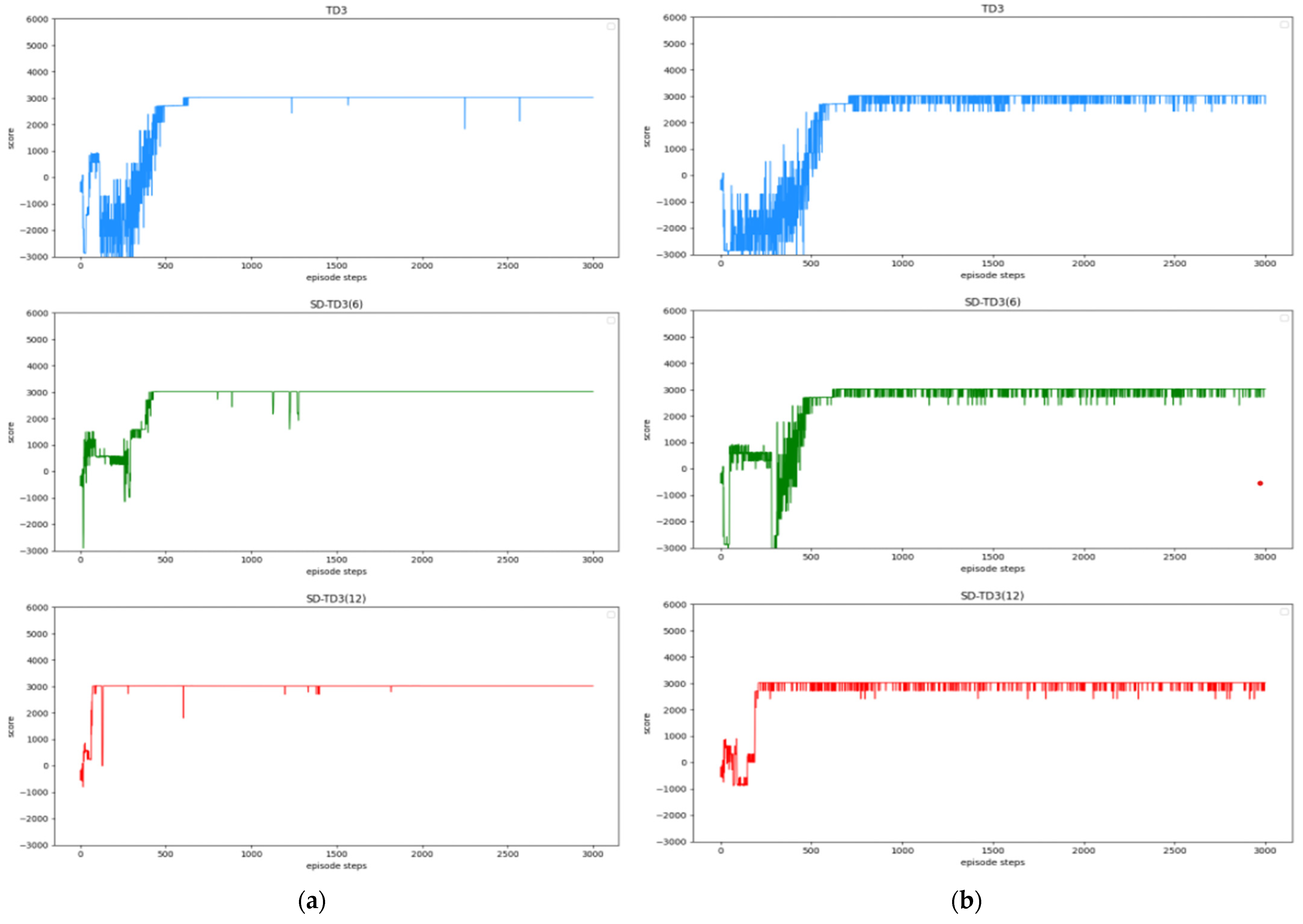
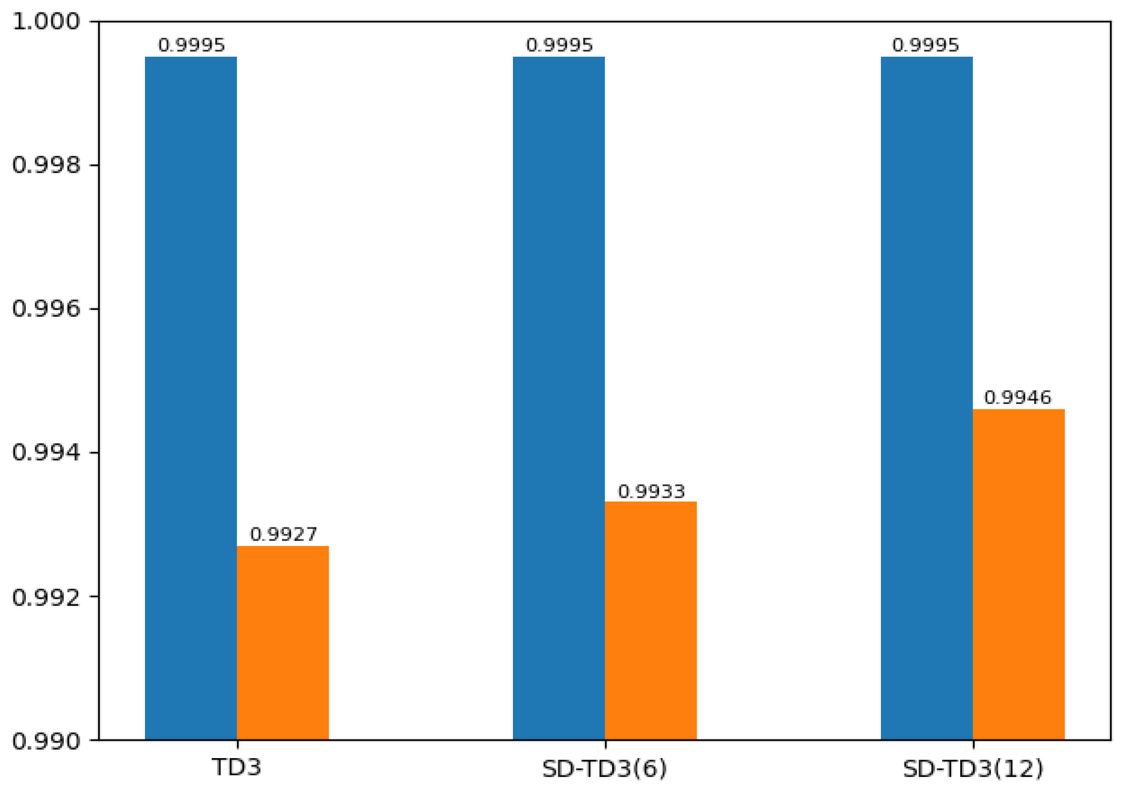
In this paper, we propose a state detection method based on the TD3 algorithm to solve the autonomous path planning problem of UAVs in low-altitude conditions. Firstly, the process of a UAV raid mission in a complex low-altitude environment was modeled, as were the static environment and dynamic environment of low-altitude flight. Similarly, in order to solve the problem of sparse reward in traditional reinforcement learning, a dynamic reward function with heuristic guidance is set up, which can make the algorithm model converge faster. On the basis of these works, combined with the state detection method, the SD-TD3 algorithm is proposed. The simulation results show that the convergence speed of the SD-TD3 algorithm model is faster than that of the TD3 algorithm model in both a static and a dynamic environment. In the static environment, the actual task completion rate of the SD-TD3 algorithm is similar to that of the TD3 algorithm, but in the dynamic environment, the success rate of the SD-TD3 algorithm model to complete the raid task is higher than that of the TD3 algorithm, and with the detailed division of the space state information in the direction of UAV travel, the success rate of the SD-TD3 algorithm model will also improve. In general, the SD-TD3 algorithm has a faster training convergence speed and a better ability to avoid dynamic obstacles than the TD3 algorithm. The SD-TD3 algorithm needs to accurately extract environmental information to determine the position of obstacles, but in practical applications, many sensors are needed to extract and process environmental information. This paper does not study the collaborative processing method of these sensors, so it will be challenging in practical applications. In future work, it can be further studied to change the input mode of the algorithm model and input more effective environmental information to promote the algorithm model’s ability to make correct decisions. At the same time, the SD-TD3 algorithm is combined and compared with other DRL algorithms, such as the PPO (proximal policy optimization) algorithm and SAC (soft actor critic) algorithm.


