Multi-Objective Optimization of a Small Horizontal-Axis Wind Turbine Blade for Generating the Maximum Startup Torque at Low Wind Speeds

Abstract

Generating a high startup torque is a critical factor for the application of small wind turbines in regions with low wind speed. In the present study, the blades of a small wind turbine were designed and optimized to maximize the output power and startup torque. For this purpose, the chord length and the twist angle were considered as design variables, and a multi-objective optimization study was used to assess the optimal blade geometry. The blade element momentum (BEM) technique was used to calculate the design goals and the genetic algorithm was utilized to perform the optimization. The BEM method and the optimization tools were verified with wind tunnel test results of the base turbine and Schmitz equations, respectively. The results showed that from the aerodynamic viewpoint, the blade of a small wind turbine can be divided into two sections: r/R < 0.52, which is responsible for generating the startup torque, and r/R ≥ 0.52, where most of the turbine power is generated. By increasing the chord length and twist angle (especially chord length) in the r/R < 0.52 section and following the ideal chord length and twist angle distributions in the r/R ≥ 0.52 part, a 140% rise in the startup torque of the designed blade was observed with only a 1.5% reduction in power coefficient, compared with the base blade. Thereby, the startup wind speed was reduced from 6 m/s for the base blade to 4 m/s for the designed blade, which provides greater possibilities for the operation of this turbine in areas with lower wind speeds.

1. Introduction

The seventh goal of the United Nations Sustainable Development is access to clean and affordable energy for all people [1]. According to the global sustainability indicators, the wind is one of the best renewable energy sources in terms of sustainability [2]. Wind turbines are employed to capture the kinetic energy of wind and convert it into electrical power. While the technology and research interest for large wind turbines are rapidly growing, small wind turbines (SWT) require further examination, since these turbines can be suitable tools for providing electricity [3], and using them is cost-effective [4].

For economic and technical reasons, SWTs do not have a pitch controller [5]. With the aid of this controller, the blade rotates around its axis and by changing the twist angle, the angle of attack is adjusted to the optimal level. Due to the absence of this mechanism in SWTs, it is not possible to optimally position the section of the blade in direction of the wind. This is especially important at low wind speeds and when SWTs begin rotating from a motionless state. Because in this state, the blade sections experience considerably high angles of attack, which result in reduced lifting force and startup torque. To solve this problem and increase the startup torque, SWTs usually have multiple blades [6]. Experimental results have shown that as the blade begins to rotate, the angles of attack decrease over time, which leads to a higher lift-to-drag ratio and as a result, raises the aerodynamic torque and facilitates the rotation and acceleration of the blade [7]. Thus, generating a high startup torque to overcome the generator resistive torque is a cardinal factor for using these turbines in areas with low wind speeds, which requires more investigation. Berges [8] employed simulation and experimental approaches to investigate the startup and performance of a decentralized electricity generation center based on SWTs in Kenya. The findings of this study indicated that SWTs are viable sources of electricity generation if they can work at low to medium wind speeds. Based on the literature, Computational Fluid Dynamic (CFD), Vortex Method (VM), and Blade Element Momentum (BEM) are common approaches that are used to predict the performance and aerodynamic forces of wind turbines. The aerodynamic behavior of SWTs was investigated in the work of Hansen and Madsen [9]. In their study, which was mostly focused on CFD and the BEM methods, they assessed various approaches for determining the aerodynamic properties of wind rotors. They regarded the BEM model as a simple yet rapid approach for calculations compared with the other aerodynamic models. They also stated that the CFD method is a great tool for verifying the designs because it has a very close agreement with experimental results.

The blade shape plays an essential role in the output power as well as the startup behavior of turbines and is generally determined by three parameters, including, the airfoil profile, and the distributions of twist angle (θ) and chord length (c) along the blade (see Figure 1). In large wind turbines, a group of airfoils is employed in various sections of the blades, each airfoil having its specific task. Thick airfoils are used near the hub to withstand structural stresses, and thinner airfoils with higher lift-to-drag (L/D) ratios are used at the blade tip to generate more power [10]. In contrast to large wind turbines, to reduce construction costs, only one airfoil is used along the blade of SWTs. These turbines typically operate at Reynolds numbers (Re) less than 500,000 [11]. Singh et al. [12] designed an airfoil specifically for application in a small horizontal-axis wind turbine (SHAWT) at low Reynolds numbers. Their modified airfoil presented significant improvements in terms of performance in comparison with other airfoils. Their findings showed that by using thin airfoils the adverse pressure gradient can be reduced on the suction side of the airfoil and consequently the aerodynamic performance of the turbine can be enhanced.

Regardless of the blade size, the θ and c profiles along the blade are determined based on the design objective or objectives. The first and most important objective in the design of a turbine blade is to achieve the maximum power coefficient (C_p) [13]. For this purpose, the analytical correlations presented in the literature [14] or optimization algorithms can be employed. In this regard, in recent years, the use of nature-inspired metaheuristic approaches to optimize wind turbine blades has substantially grown. As the name suggests, these algorithms are inspired by the behavior of animals or other natural processes. Some examples of popular nature-inspired metaheuristic algorithms are Cuckoo Search [15], Jumping Frogs Optimization [16], Bat Algorithm [17], Genetic Algorithm (GA) [18], Ant Colony Optimization [19], and Particle Swarm Optimization [20]. Soni et al. [21] compared the performance of twelve types of nature-inspired algorithms from the perspectives of accuracy, speed, convergence, and efficiency. Their results showed the GA provides rapid speed and also a great accuracy. This point has caused the widespread use of this algorithm for optimizing wind turbine blades [22,23].

Hassanzadeh et al. [13] increased the output power of a SHAWT by more than 8.5% by optimizing the θ and c profiles of its blade. The design and optimization of SWT blades for improving their C_p and startup time (T_s) has been carried out by Wood [10] and Pourrajabian et al. [22]. The results have shown that increasing the θ and c in the root region can reduce the T_s of the turbine. In another study, Pourrajabian et al. [24] suggested the use of hollow blades to reduce the blade inertia (J) for reducing the T_s of SWTs. Akbari et al. [25] investigated the effect of ten different airfoils on the performance of an SWT in terms of T_s and C_p. The results showed that SG6043 and BW-3 airfoils have the best performance in windy regions and regions with low wind speeds, respectively. The optimization of the control systems [26], minimizing mass [27], cost [23], and aerodynamic noise [28] are some of the other design and optimization objectives of wind turbine blades that have been examined by researchers.

Abdelsalam et al. [29] investigated the effect of linear and nonlinear θ and c profiles on the performance of an SWT with a rotor diameter of 1 m at wind speeds of 5–10 m/s. The results showed that the maximum C_p of linear and nonlinear models is 0.426 and 0.446 respectively. The blade with a linear distribution started to rotate at a wind speed of 5 m/s, while this value for the blade with a nonlinear distribution was found to be 6 m/s. Rector et al. [30] investigated the effect of solidity, the number of blades (N = 3, 6), and pitch angle on the performance of a SHAWT. The results showed that by increasing the solidity and the number of blades, the turbine performance improves at low wind speeds, but the rotor with three blades performs better at high wind speeds. The results of Eltayesh et al. [5] revealed that raising the number of blades reduces the maximum C_p and blade tip speed ratio, but it raises the startup torque and reduces the required wind speed for the start of the rotation. Similar results were observed in the research conducted by Wang and Chen [31]. In the recent study by Bourhis et al. [6], it was highlighted that with a fixed number of blades (N = 8), the increase in solidity due to the increase in the c leads to a better startup torque. They showed that by raising the solidity from 0.5 to 1.25, the required wind speed for the start of rotation is decreased from 5.8 m/s to 3.8 m/s. In their study, the effect of θ on the startup torque was not studied, while according to the work of Astolfi et al. [32], the θ is one of the most effective parameters in the startup process of wind turbines.

Based on the literature review, it can be observed that so far, to improve the startup performance of SWTs, researchers have mostly focused on increasing the number of blades and reducing the blade inertia and startup time. On the other hand, the startup torque capabilities have drawn less attention. Therefore, in the present study, an attempt is made to investigate the effect of the geometrical shape of the blade on the startup torque of an SWT. In this regard, the twist angle and chord length were chosen as the design variable, and to determine their distributions along the blade, a multi-objective optimization algorithm was used to maximize the output power as well as the startup torque. Indeed, in the current research, an attempt is made to answer the question that without increasing the number of blades and only by changing their geometrical shape, to what extent it is possible to increase the startup torque of a stationary blade so that the output power of the turbine does not drop significantly? The BEM method was employed to perform the relevant calculations and a genetic algorithm was used to perform the optimization process.

2. The Base Wind Turbine

The SHAWT that is examined in the present study was designed and experimentally assessed by Anderson et al. [33]. Figure 2 illustrates the geometrical presentation of this two-bladed turbine. A NACA4412 airfoil is employed as the profile of the blade. The geometry of this airfoil is illustrated in Figure 3. It is noteworthy that the NACA4412 airfoil was originally designed for application in the aviation industry, but due to the simplicity of its fabrication process, it has become one of the most popular airfoils in SWTs [34].

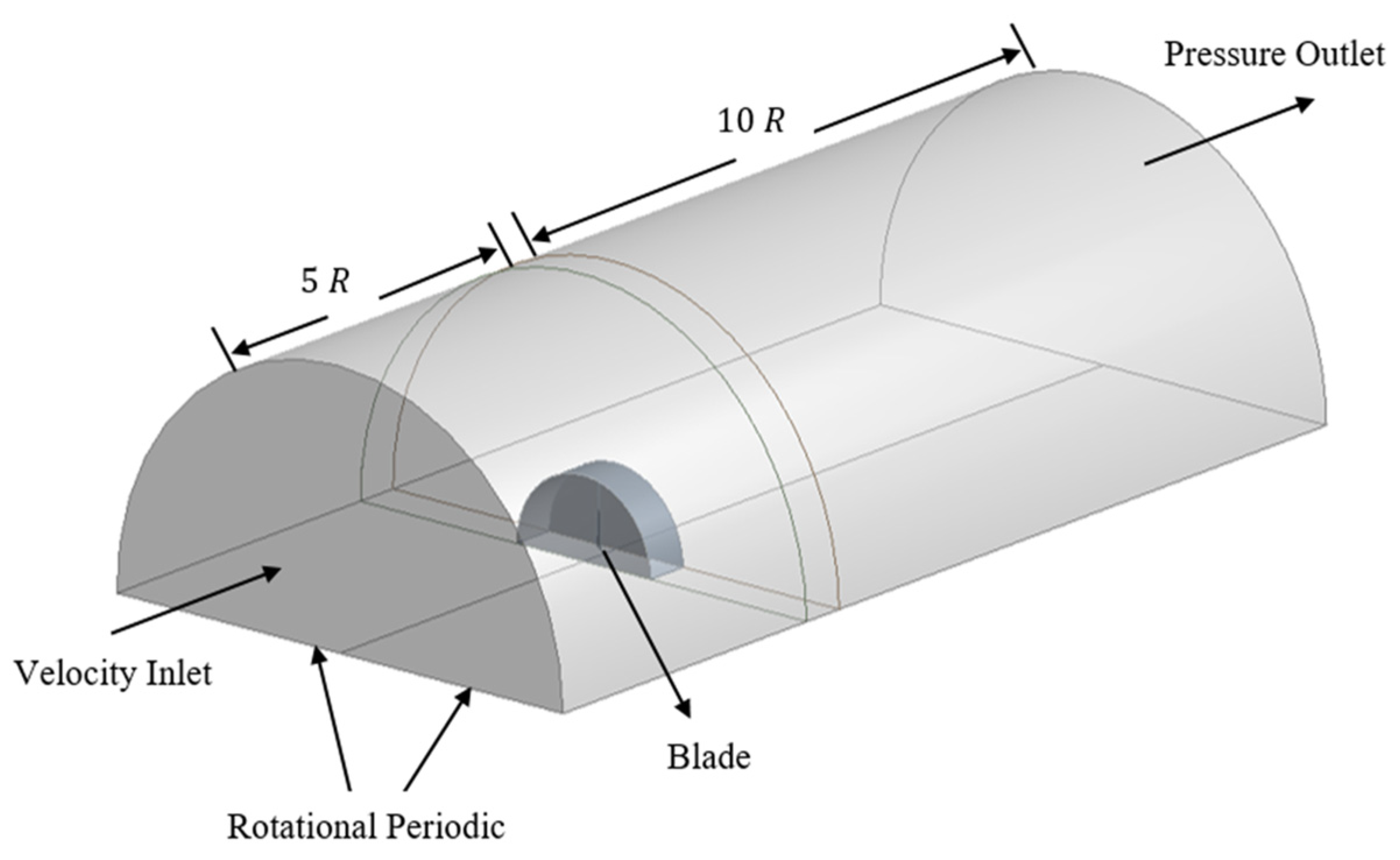
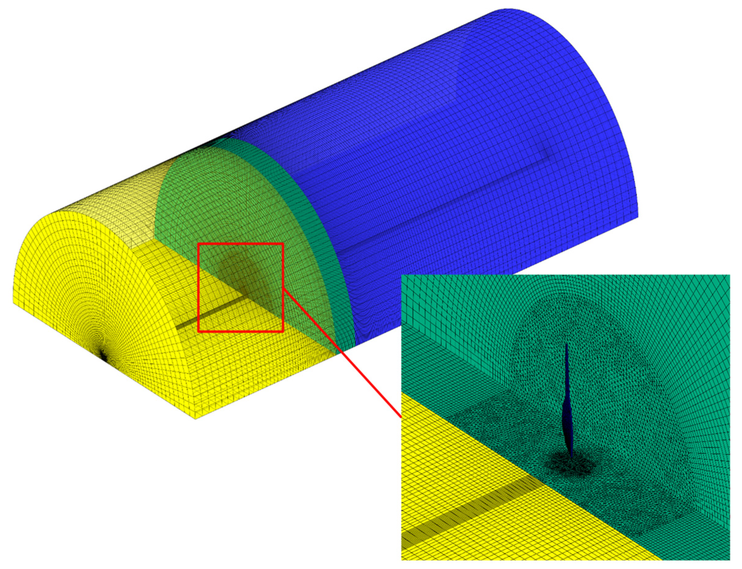
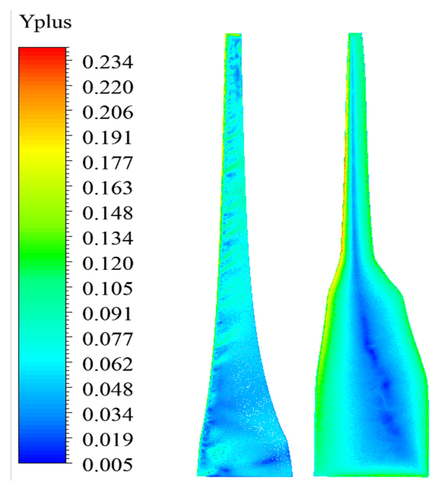
3. Numerical Methodology

3.1. Calculating Design Goals

The BEM method was employed to calculate the C_p as well as the startup torque. This method was proposed by Glauert [35] in 1935 [14,36]. In the BEM, the blade is separated into various individual elements, which have a particular θ and c values. Using conservation laws, including the continuity correlation and the momentum correlations for these elements, the amount of local forces is computed for the entire blade, and by summing the loadings along the blade, the total torque (Q) is obtained which is employed to calculate the C_p as follows:

$$C_p=\frac{Q\omega }{0.5\rho S{U}^3}$$

(1)

where, $\omega$, $\rho$, S, and U indicate the rotational velocity, air density, the blade swept area, and the wind speed, respectively. To consider the tip losses, Prandtl’s tip loss correction factor was used in the BEM calculations. This correction model (F) which is a function of the blade number (N), the flow angle (ϕ), and the local radius (r) is defined as follows [37]:

$$F=\frac{2{\cos }^{-1}\left(e^{-f}\right)}{\pi }$$

(2)

$$f=\frac{N\left(R-r\right)}{2r \sin \varphi }$$

(3)

$$\varphi =\theta +\alpha$$

(4)

in which, α represent the angle of attack.

When the blade is stationary, α values are higher than 20° in its sections [24], in which case these parts behave like flat plates from an aerodynamic viewpoint; therefore, the analytical lift and drag coefficients can be used in the startup analysis with satisfactory precision [38].

$$C_l=\sin 2\alpha$$

(5)

$$C_d=2 {\sin }^2 \alpha$$

(6)

By using Equations (5) and (6) in the BEM theory, the startup torque (Q_s) can be calculated as follows [24]:

$$Q_S=N\rho U^2{R}^3\underset{r_h}{\overset{1}{{\displaystyle \int }}}{(1+{\lambda }_r{}^2)}^{1/2}cr sin\theta \left(cos\theta -{\lambda }_{r}sin\theta \right)dr$$

(7)

where $r_h$, and ${\lambda }_r=\frac{r}{R}\lambda$ are the hub radius, and the local tip speed ratio respectively. In this equation, all dimensions and speeds are normalized based on the R and the wind speed (U), respectively. By inserting $\lambda =0$ in Equation (7), the value of the Q_s on a stationary blade can be calculated.

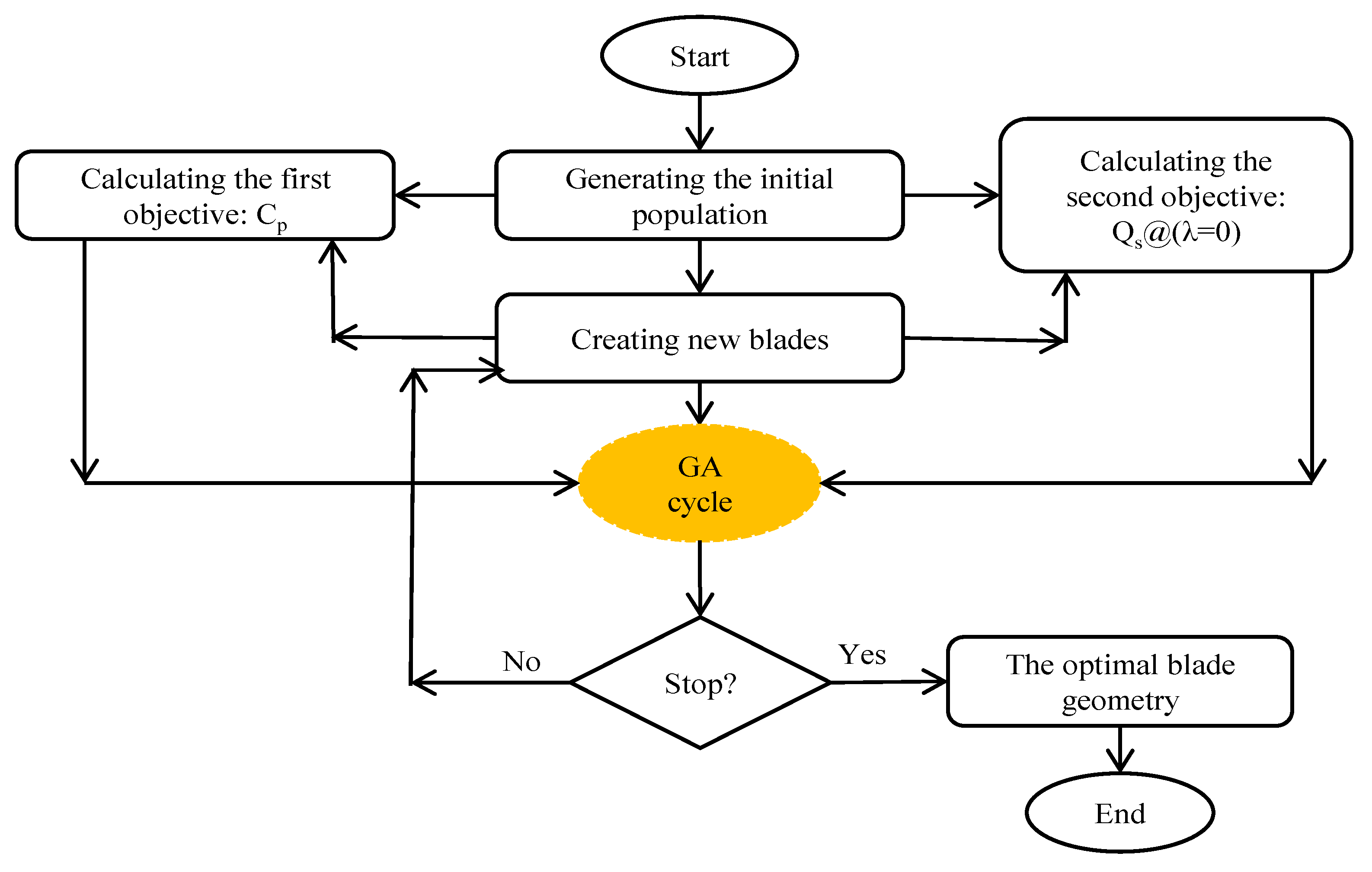
3.2. Multi-Objective Optimization

To determine the geometry of the optimal blades, the genetic algorithm method was used. Inspired by natural evolution, this algorithm was introduced by Holland [39] in 1975 and developed by Goldberg [40]. The results have shown that this algorithm has a good performance in the multi-objective optimization of wind turbine blades [24]. To find the optimal solutions, in the genetic cycle, three operators including, selection, crossover, and mutation are used one after another. The operation method is that at first, the primary population matrix, which includes chromosomes that are the candidate solutions or design variables, is created completely randomly. Each row of this matrix represents a blade. Subsequently, based on the value of the objective function, the best ones are selected as parents by the selection operator to produce children which may have a better objective function value with the help of the crossover operator. In the end, the mutation operator is used to prevent the algorithm from converging to the local solutions [41]. All these steps are repeated for a large number of generations until finally an optimal and global solution is obtained.

To achieve the two objectives that were previously mentioned, i.e., maximizing the C_p and Q_s, the following equation was considered as the objective function:

$$Maximize:\left(n\frac{C_P}{\max \left(C_P\right)}+\left(1-n\right)\frac{Q_s}{\max (Q_s)}\right)$$

(8)

where n is the parameter that determines the weight of each design goal in the objective function. The terms, $\max \left(C_P\right)$ and $\max \left(Q_s\right)$ are the maximum C_p and the maximum Q_s of the blades, respectively.

3.3. Configuring the Input Variables

Figure 4 shows a flowchart for the proposed optimization algorithm.

To perform the optimization, it is necessary to determine the value of the tip speed ratio ($\lambda$) at which the base turbine reaches its maximum C_p at a rated wind speed of 10 m/s. According to the experimental test results of this turbine, which are mentioned in the results section (validation of the BEM code), this value is equal to 10.16. The wind speed for the startup process was set at 5 m/s. It is noteworthy that although changing the startup wind speed ($U_s$) can completely alter the Q_s, it does not affect the geometric shape of the optimal blades because Equation (7) is independent of the Reynolds number. The considered range for the design variables based on the fabrication restrictions is listed in

Table 1. The considered range for the design variables [24].

Variable	Lower Limit	Upper Limit
$\theta$ (°)	−5	25
c/R	0.01	0.2

.

Twenty elements were considered along the blade; thereby, the number of the design variables in the genetic algorithm is 40.

Table 2. The input values in the GA [22].

Variable	Value
Population	3000
Number of generations	500
Selection rate	0.1
Mutation rate	0–0.1

shows the input parameters considered in the genetic algorithm.

4. Results and Discussion

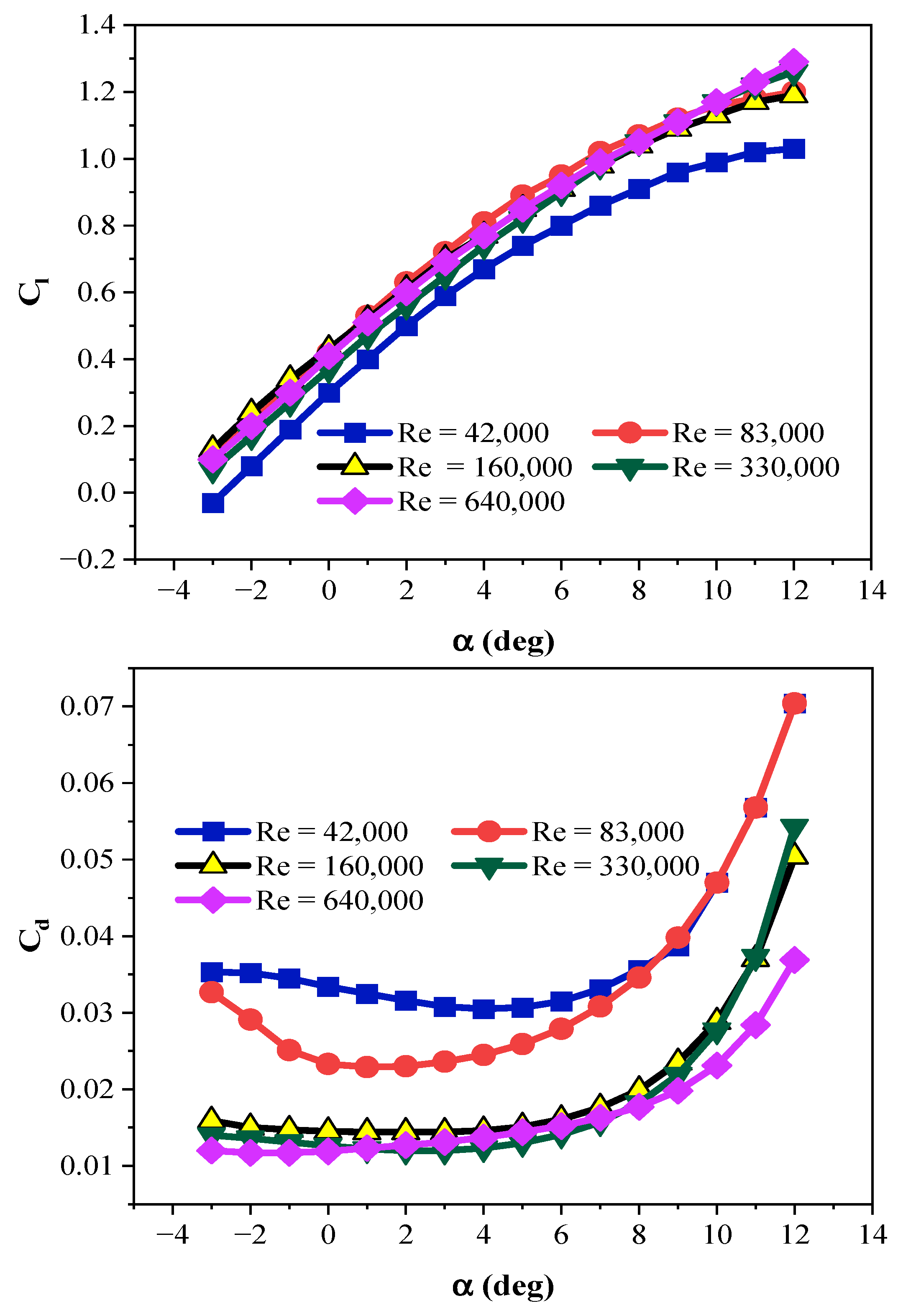
4.1. Validity of the BEM Technique

To check the validity of the BEM technique, this section compares the experimental data of the base turbine from the wind tunnel test with the data acquired for the current research. The drag and lift (C_d and C_l) coefficients of the NACA4412 profile, at different α and various Re numbers, are shown in Figure 5. These coefficients are tabulated and considering the Re and α of each element, the related lift, and drag values are calculated and called in the BEM and also optimization stages.

Figure 6 illustrates the $C_P$ alternations at various tip speed ratios ($\lambda$). By considering this figure, it can be noticed that the values acquired by the numerical code are in satisfactory agreement with the wind tunnel test data with a maximum deviation of 6.5%.

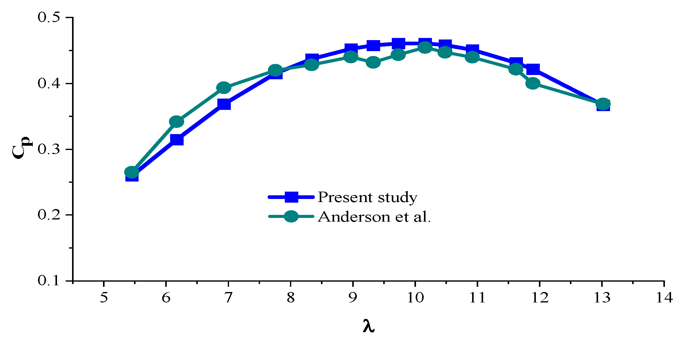
4.2. Validity of the Optimization Technique

The Schmitz formula [42] was utilized to examine the efficiency of the optimization code. By taking the air circulation behind the blade into account, and neglecting the drag and tip losses, these equations specify the distribution of $\theta$ and $c$ along the blade to achieve the maximum C_p.

$$\theta =\frac{2}{3}{\tan }^{-1}\left(\frac{1}{{\lambda }_r}\right)-\alpha$$

(9)

$$c=\frac{16\pi r}{N{C}_{l }} si{n}^2 \left(\frac{1}{3} {\tan }^{-1}\left(\frac{1}{{\lambda }_r}\right)\right)$$

(10)

To use these correlations, C_l and α should be determined at the maximum L/D ratio. For the NACA4412 airfoil, at $\mathrm{Re}=3\times {10}^5$, these values are 6° and 0.9, respectively [10]. By placing n = 1 in the objective function (Equation (8)), the distributions of $\theta$ and $c$ which are obtained from the optimization algorithm are compared with those from the ideal correlations (Equations (9) and (10)) in Figure 7.

As can be observed, the distributions are very close to each other, so it can be ensured that the final answer obtained from the optimization code is an optimal solution.

4.3. Performing the Optimization

By taking the conditions specified in Section 3.3 of the study into account, the optimization process was employed to design the optimal blades. In multi-objective optimization problems, more than one candidate answer exists for the designer, in which case the Pareto front is used to determine the best answer. Figure 8 shows the Pareto front for the $C_P$ and $Q_s$. As can be observed, the blade that generates the maximum power (n = 1) has the lowest $Q_s$. As the value of the n parameter decreases, the importance of the $Q_s$ in the objective function increases, which results in a reduction of the $C_P$. This is a trend that should be expected because in multi-objective optimization problems, concentrating on one objective weakens the other objective/objectives. However, it is worth noting that with a slight reduction in the $C_P$, a significant increase in the $Q_s$ is observed (see Figure 8).

Figure 8 illustrates the important point that the design of SWT blades has to be according to the wind potential of the region where it is going to be employed. Considering this, in windy areas where the aim of designing wind turbine blades is to reach the maximum C_p, the blades with n = 1 and n = 0.95 are recommended, while the blade with n = 0.75 is the best choice for generating a high Q_s for areas with low wind speeds. Figure 9 shows the distribution of $\theta$ and $c$ for the optimal blades.

As can be observed, by decreasing the n value, the optimization algorithm considers higher values for θ and c (especially c) for the inner part of the blade (r < 0.52). There are two reasons for this, which are discussed here. First, as mentioned in Section 3.1, when the blade is stationary, its sections experience high angles of attack. Therefore, one way to reduce them is to increase θ. Second, Equation (7), which was used to calculate the Q_s, is in direct relationship with c. Thus, the optimization algorithm tries to increase Q_s by raising c, of course in the design limit that was specified in Table 1. But the remarkable point regarding Figure 9 is that the shape of the blades is considerably similar at r/R ≥ 0.52, the reason for which is explained in detail in Section 4.4.

Since the present study aims to design a blade with a high Q_s to work at low wind speeds, the blade with n = 0.75 is selected as the optimal blade for further analysis. It should be noted that the blade with n = 0.7 was also considered in the objective function, but the optimization algorithm could not produce a smooth distribution for θ and c in the outer part of the blade. Because by reducing n in Equation (8), the optimization algorithm mostly focuses on the evolution of design variables on the inner part of the blade to raise the Q_s, which results in discrepancies in the outer part of the blade and a sharp reduction in the C_p. Thereby, it was ensured that the blade with n = 0.75 is the most suitable blade based on the design objectives.

Figure 10 compares the θ and c profiles of the optimal blade from the current study (with the objectives of maximizing the C_p and maximizing the Q_s) and the optimal blade designed for a 0.75 kW turbine by Pourrajbian et al. [24] (with the goals of maximizing the C_p and minimizing T_s).

As can be observed, c and θ distributions determined by Pourrajbian et al. have many discrepancies, which makes the blade manufacturing process impossible. In this situation, it is necessary to use the polynomial curve for fitting the results [10]. This issue takes the blade away from its optimal condition. The blade designed in this research does not have these discrepancies and will be examined and compared with the base blade in both CFD and BEM calculations with the same geometry. It is necessary to explain that the results of the present study show that from the aerodynamic viewpoint, the blade is divided into two completely different areas. The first half is responsible for creating Q_s and requires an increase in θ and c values, and the second half is responsible for generating the output power; for that part, the θ and c profiles can be obtained from ideal correlations.

4.4. The Power Generation Analysis

The purpose of this section is to further investigate the flow field around the base/designed blades using CFD beside the BEM analysis. In this regard, the C_p, as well as the aerodynamic torque generated along the blades, is examined. Figure 11 shows the geometry of the base and designed blades.

The steady-state, RANS form of governing equations, and Shear Stress Transport (SST) k-ω turbulence model were considered for the simulations that were carried out for the base/designed blades using the ANSYS Fluent software [43]. The second-order upwind technique was used to discretize the convection terms and a semi-implicit (SIMPLE) method was employed for the pressure-velocity coupling.

To reduce the computational cost, by applying a periodic boundary condition only one blade was modeled. The computational domain and the chosen boundary conditions are shown in Figure 12.

The domain was $\mathrm{½}$ of a cylinder (180° sector) and was divided into two zones: the blade zone and the outer zone. The boundary conditions were set as follows: velocity inlet for the inlet (located 5R upstream), pressure outlet for the outlet (located 10R upstream), symmetry for the outer boundary, periodic for the lateral planes, a solid wall with a no-slip condition for the blade surface, and interface for merging the separated frames. Additionally, the moving reference frame model was employed to simulate the rotation.

The precision of a CFD simulation depends on the quality of the generated mesh. Due to the complexity of the blade geometry, an unstructured mesh was used for the blade zone while because of the simple geometry of the outer zone, a structured mesh was applied for that region. Figure 13 depicts the mesh generated for the computational domain.

To improve the accuracy of the calculations in the boundary layer, a prism layer was created to cover the blade surface. Since the SST k-ω model needs $y^{+}<1$, the height of the first layer was considered to be $1\times {10}^{-6}$. Figure 14 shows the $y^{+}$ distribution contours on the suction side of the base/designed blades.

The grid-independency check was carried out by testing grids with different densities. The torque generated by the blades was selected as the basis to judge the grid-independency test results.

Figure 15 shows these results. Grids with $8.8\times {10}^6$ and $11.9\times {10}^6$ elements were selected for the base and designed blades, respectively.

Table 3. The C_p values of the base/designed blades.

Method	${\mathit{C}}_{\mathit{p}}$
	Base Blade	Designed Blade
Anderson et al. [33]	0.454	-
BEM	0.460	0.453
CFD	0.453	0.451

lists the C_p values obtained by the BEM and CFD methods for the base/designed blades. This table also shows the experimental C_p of the base turbine. Both methods predict a slight reduction in the C_p of the designed blade compared with the base blade, but this reduction is not noticeable, especially in the CFD method. The BEM technique, which is the basis of the present study calculations, predicts only a 1.5% reduction.

Figure 16 shows the aerodynamic torque generated during power generation in each element (20 elements) for the base/designed blades. As can be observed, the trend of changes in the generated torque in the two methods is very close.

The aerodynamic torque increases along the blade from the hub to $r/R=0.89$, but then decreases in $r/R>0.89$. The reason is the formation of tip vortices in this area of the blade. The influence of this three-dimensional phenomenon was considered by Prandtl’s tip correction factor (F) in the BEM method (see Section 3.1), but, the significant point is that the CFD results predict a greater tip loss compared with this correction factor. Figure 17 shows the tip vortices and Figure 18 presents the tip streamlines for the base/designed blades.

Tip vortices are the source of induced drag and they reduce the generated torque. These vortices are created because of the formation of a 3D spanwise flow due to the pressure difference between the pressure side and the suction side of the blade. It should be noted that the lower value of c at the tip of the designed blade slightly reduces the tip vortices compared with the base blade. One of the best ways to reduce these vortices is to use a winglet, which increases the kinetic energy captured by the blade by shifting the tip vortices from the blade tip to the winglet tip.

As mentioned in Section 4.3, the shapes of all the optimal blades are very close in $r/R\ge 052$. The reason is specified in this section. Since, according to Figure 16, most of the aerodynamic torque, which is used to generate power, is generated in the outer half of the blade, to maintain power, the optimization algorithm minimizes the changes in this part of the blade, even at low n values. This prevents a considerable reduction in power generation.

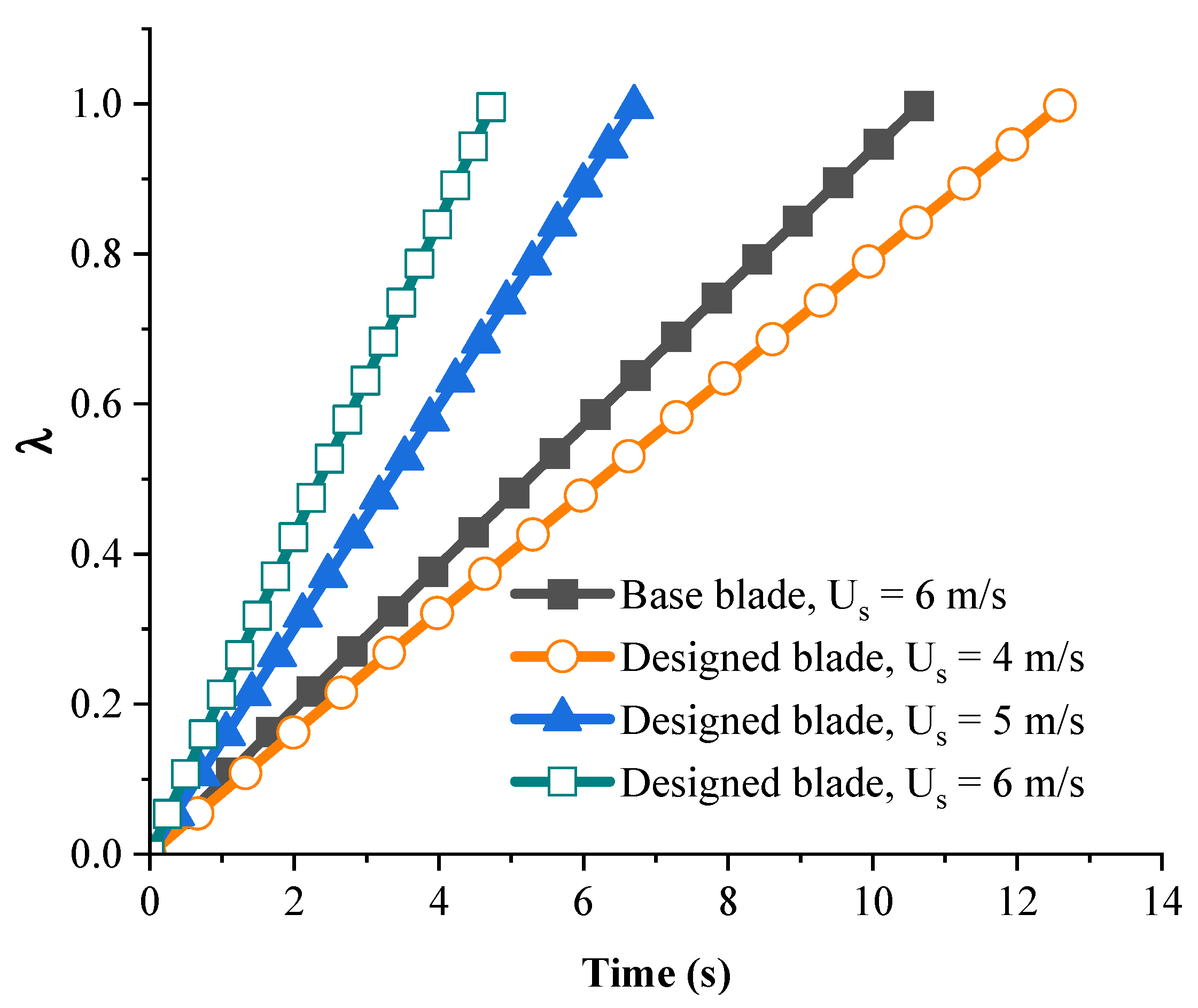
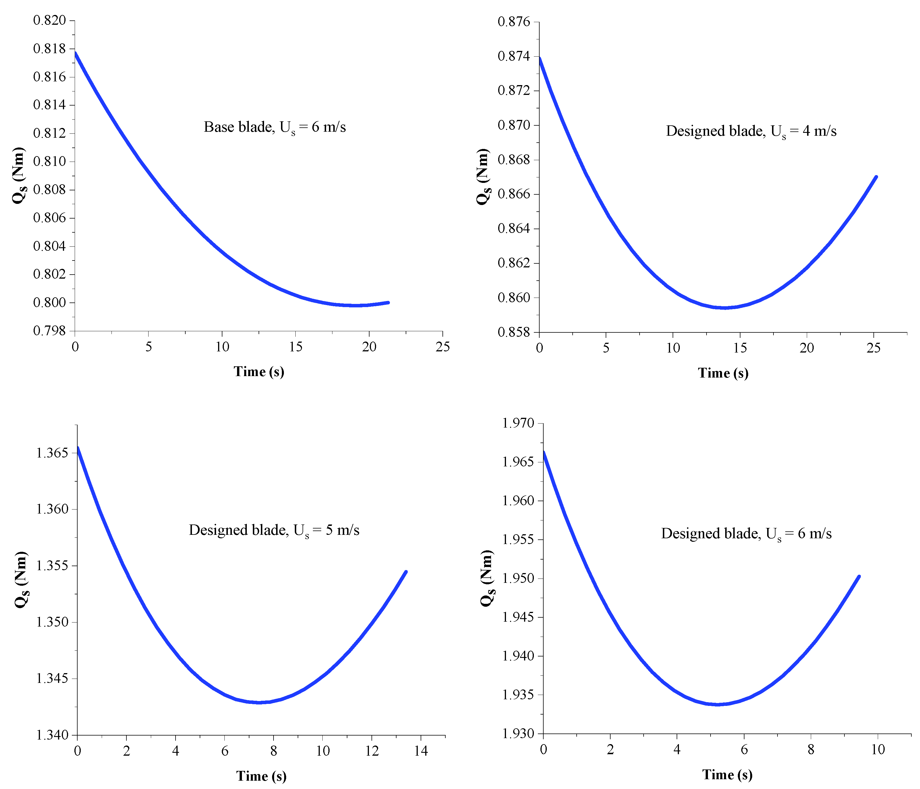
4.5. The Startup Behavior Analysis

Compared with the design condition, in which the blade elements have small and medium angles of attack, when the blade is stationary, the angles of attack are very high. Therefore, as mentioned before, Equation (7) is employed to analyze the startup process. It is necessary to explain that the analytical aerodynamic coefficients in this equation have acceptable results compared with the wind tunnel test analyses conducted at different Reynolds numbers and high angles of attack (See ref. [10]). According to this, the Q_s value of the base/designed blades is shown in Figure 19. The results show a 140% increase in the value of this parameter for the designed blade compared with the base blade. For further examination, the distribution of Q_s generated by each element is shown in Figure 20. By observing this figure, it is clear that most of the Q_s is generated in the inner half of the blade ($r/R<0.52$).

The interesting point is the negative Q_s in the tip elements of the blades, which is due to the negative θ in this region. Another parameter that has a cardinal role in the operation of SWTs at low wind speeds is T_s [24]. Indeed, generating a high Q_s becomes sensible as a practical improvement when the turbine has a low T_s so that power generation is not delayed. Raising the c in the inner part of the designed blade increases its moment of inertia, which can affect the rotational acceleration and hence the T_s of the turbine. Thereby, it is necessary to perform a T_s analysis. In this regard, the changes in $\lambda$ over time during the startup process can be considered as follows [24]:

$$\frac{d\lambda }{dt}=\frac{R\left(Q_s-Q_r\right)}{J{U}_s}$$

(11)

where, $Q_r$ is the resistive torque of the generator and $J$ is the blade moment of inertia, which can be calculated using the following correlation if all the lengths are normalized by R [22]:

$$J=N{\rho }_{b}A{R}^5\left[{{\displaystyle \int }}^{}{\left(cr\right)}^{2}dr+\frac{1}{12}\left({{\displaystyle \int }}^{}{c}^{4}co{s}^2\theta dr+A^2{{\displaystyle \int }}^{}{c}^{4}si{n}^2\theta dr\right)\right]$$

(12)

where, ${\rho }_b$ is the blade density, and A is the surface of the airfoil profile, the value of which for the NACA4412 airfoil is 0.082 ${\mathrm{m}}^2$ [10].

It is necessary to explain that the precision of Equation (11) was experimentally verified by Sessrego and Wood [44]. By solving this equation, from the stationary state to $\lambda =1$, the T_s is calculated [10]. In this study, the Adams–Moulton method was employed to calculate this equation, and the trapezoidal integration technique was used to calculate the blade inertia (Equation (12)). By considering ${\rho }_b=550 \mathrm{kg}/{\mathrm{m}}^3$ and also $Q_r=0.5 \mathrm{Nm}$ for the turbine of the present study [10,33], the T_s of the base/designed blades was investigated. The results are summarized in

Table 4. The T_s values of the base and designed blades at various wind speeds.

Case	J (kg·m2)	Ts (s)
		Us = 4 m/s	Us = 5 m/s	Us = 6 m/s
Base blade	0.798	-	-	10.63
Designed blade	1.691	12.59	6.69	4.71

for various wind speeds. In this table, the J values of the blades are also given.

As can be observed in this table, the base turbine is not able to rotate at wind speeds (U_s) of 4 and 5 m/s. On the other hand, the designed blade, despite having a higher J than the base blade, starts to rotate at U_s = 4 m/s and can be used to generate power. Figure 21 shows the changes of $\lambda$ during the startup process and Figure 22 shows the changes of Q_s up to $\lambda =2$ for the base and designed blades.

As shown in Figure 22, as the blade starts rotating, regardless of its geometry, at first, the Q_s slightly diminishes and then begins to rise. It should be noted that although the Q_s of the designed blade at U_s = 4 m/s is greater than the Q_s of the base blade at U_s = 6 m/s (see Figure 22), it has a higher T_s than the base blade. This is due to the lower J value of the base blade.

5. Conclusions

The design and optimization of the blades of an SWT with a rotor diameter of 3 m were carried out not only to reach the maximum power coefficient (C_p) but also for the maximum startup torque (Q_s) because these turbines usually lack a pitch control mechanism to adjust the optimal angle of attack. For this purpose, a genetic multi-objective optimization algorithm was employed. The twist angle (θ) and chord length (c) were considered as the design variables and the BEM method was utilized to calculate the design objectives. Validation studies were carried out for both the BEM technique and also the optimization algorithm. A weighting factor was used to make a compromise between the C_p and the Q_s, and different blades were designed by changing it. The outline of the research can be highlighted as follows:

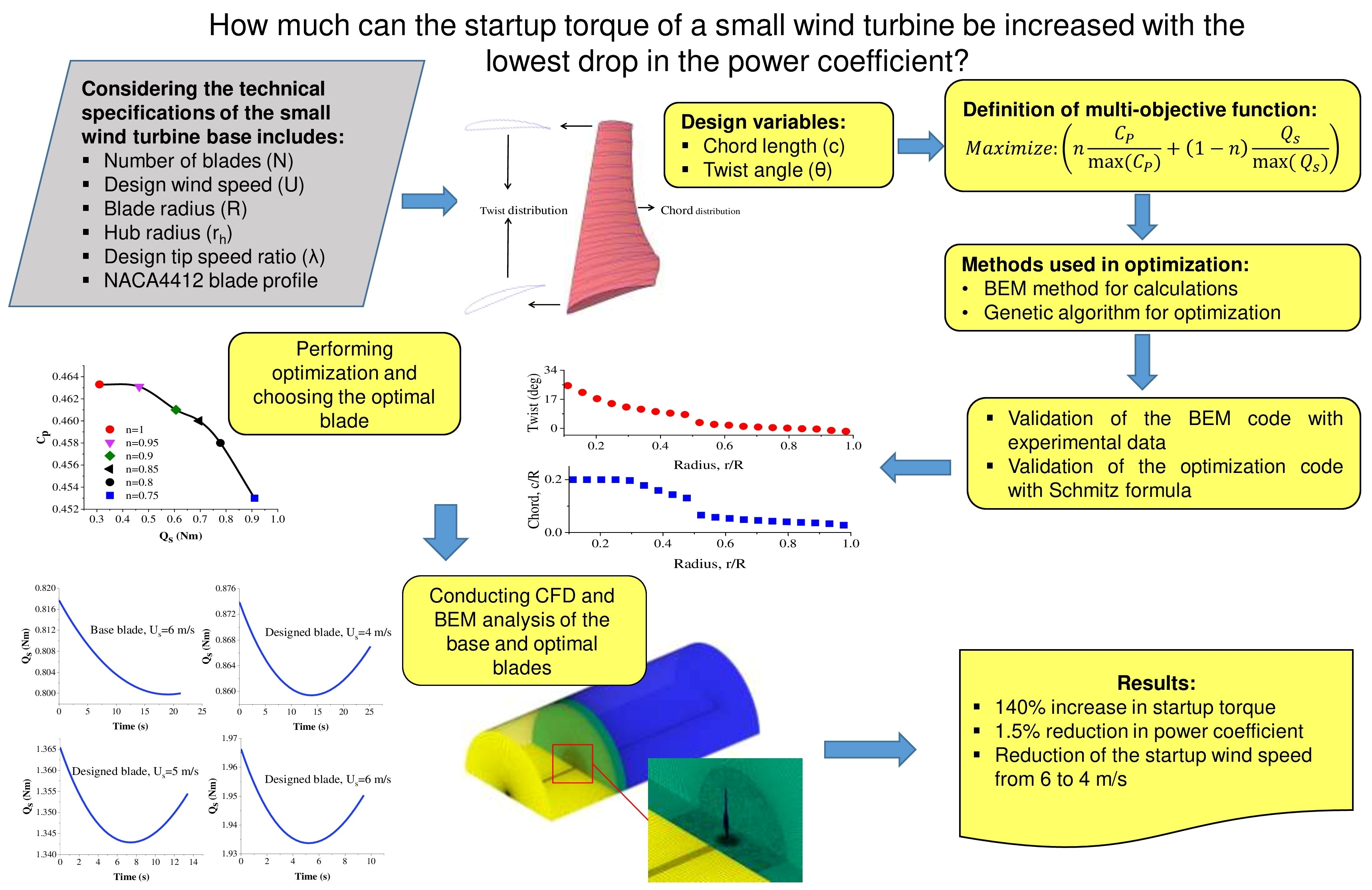
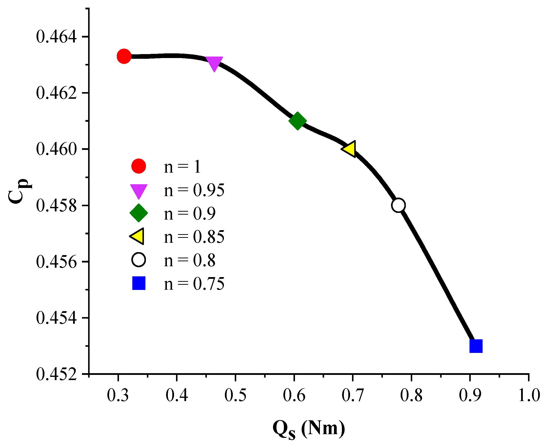
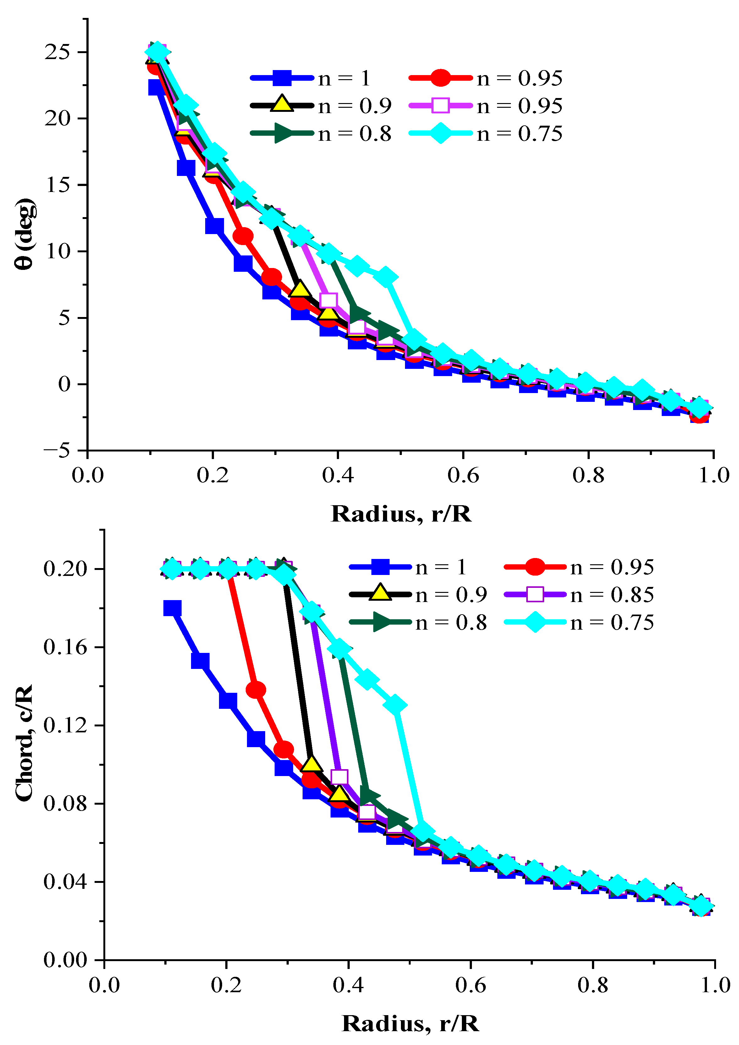
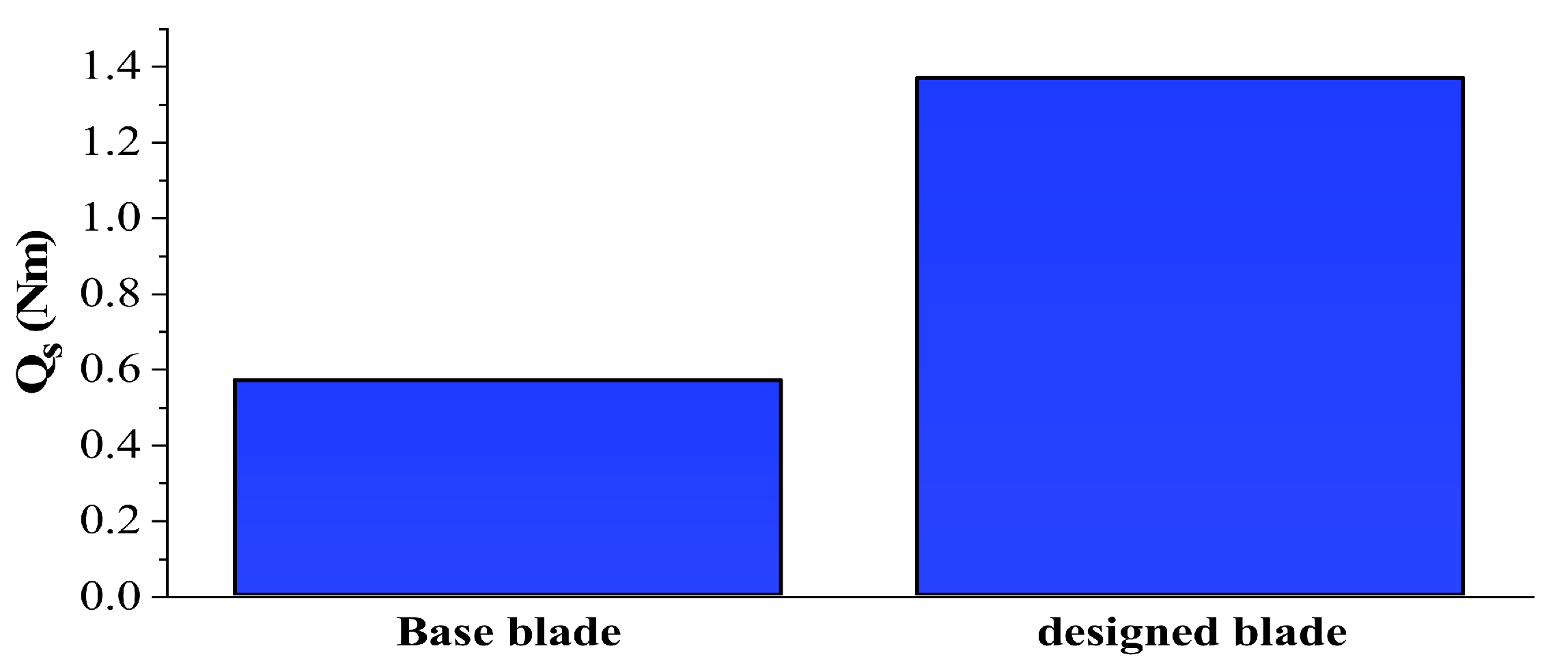
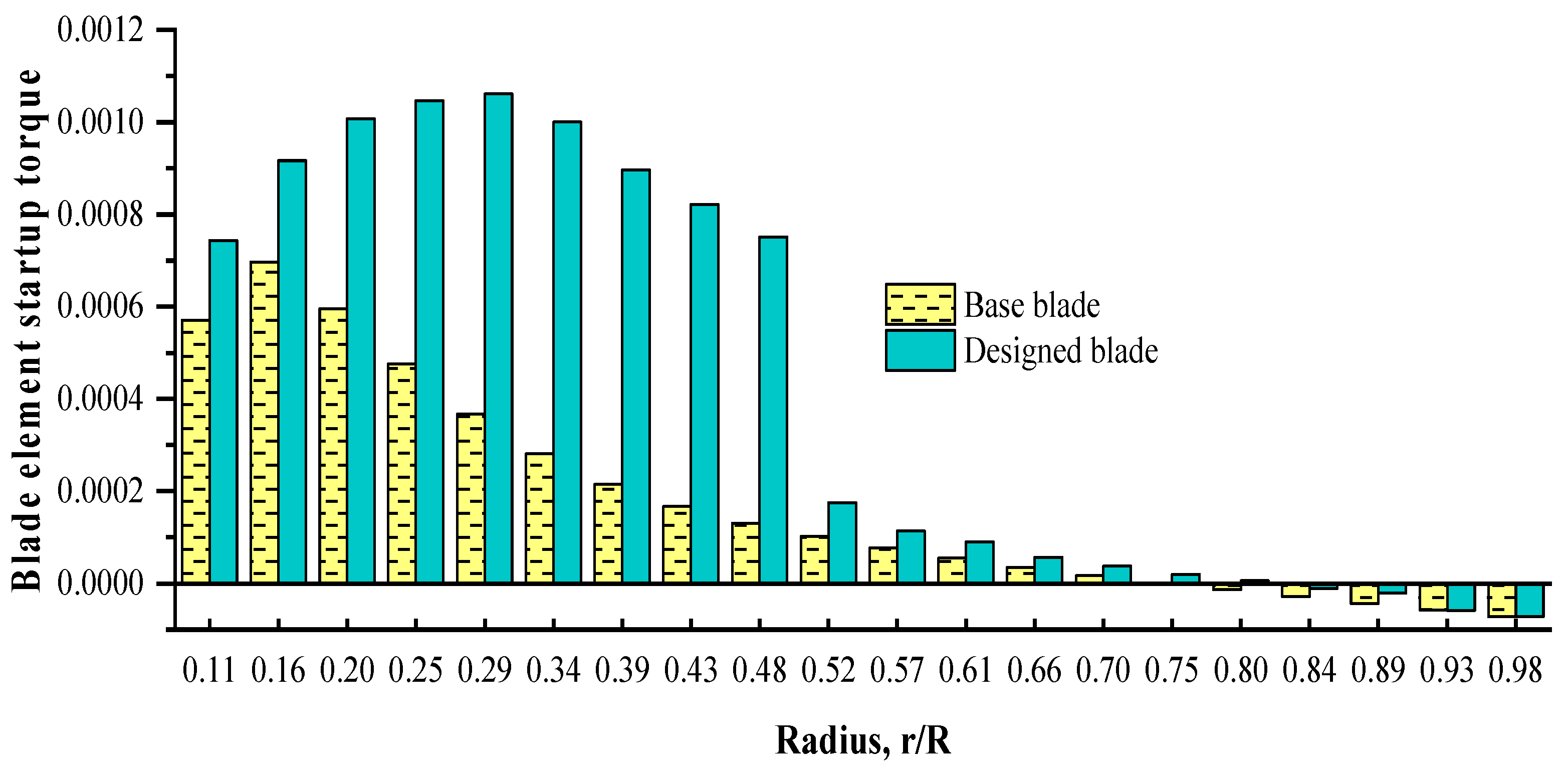
• By increasing the c and θ values in r/R < 0.52 and also following the ideal c and θ profiles in r/R ≥ 0.52, with only a 1.5% reduction in the C_p, the Q_s of the designed blade was augmented by 140% compared with the base blade. This increase in the Q_s reduced the startup wind speed from 6 m/s in the base blade to 4 m/s in the designed blade. This makes the turbine appropriate to use in more regions;
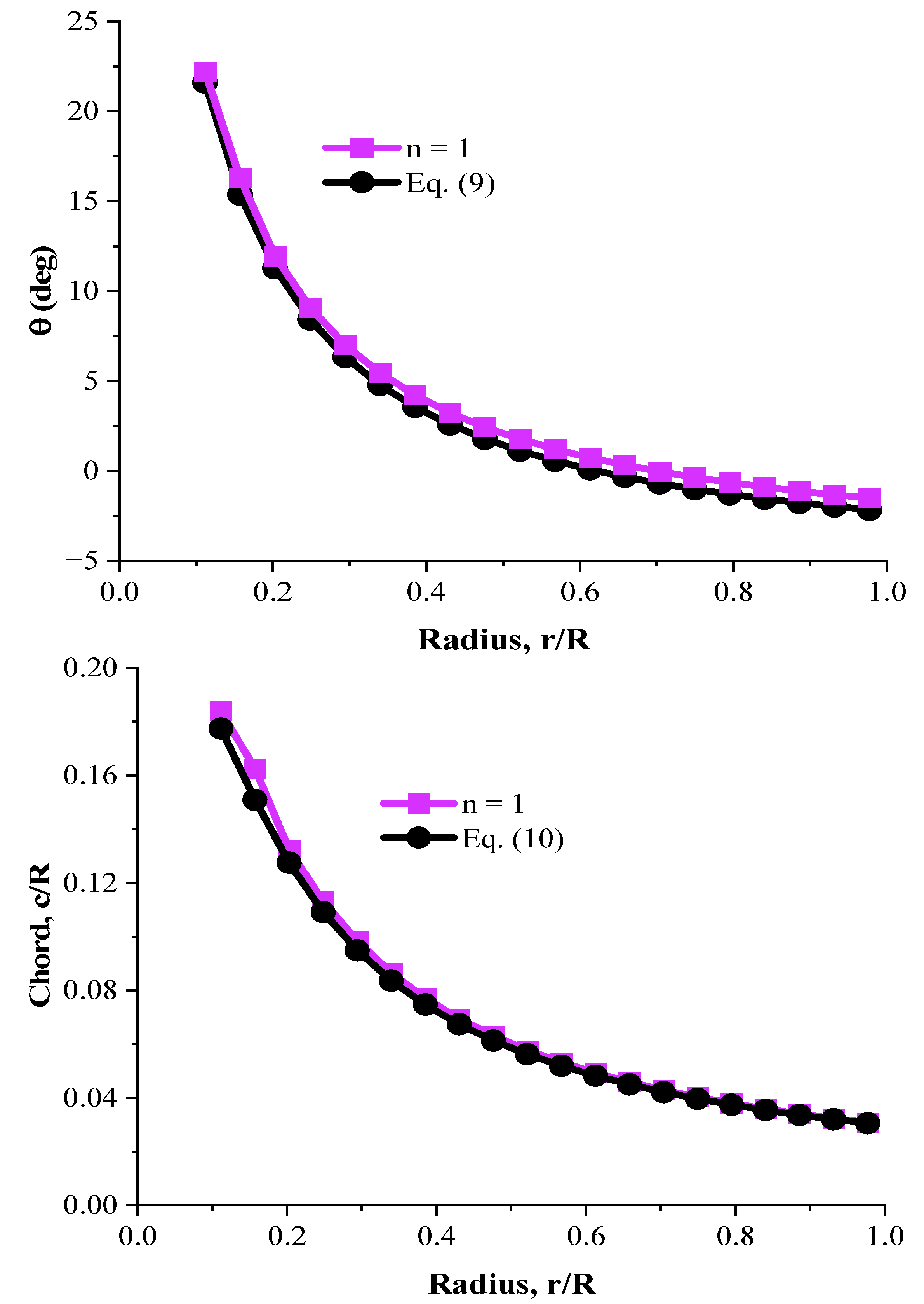
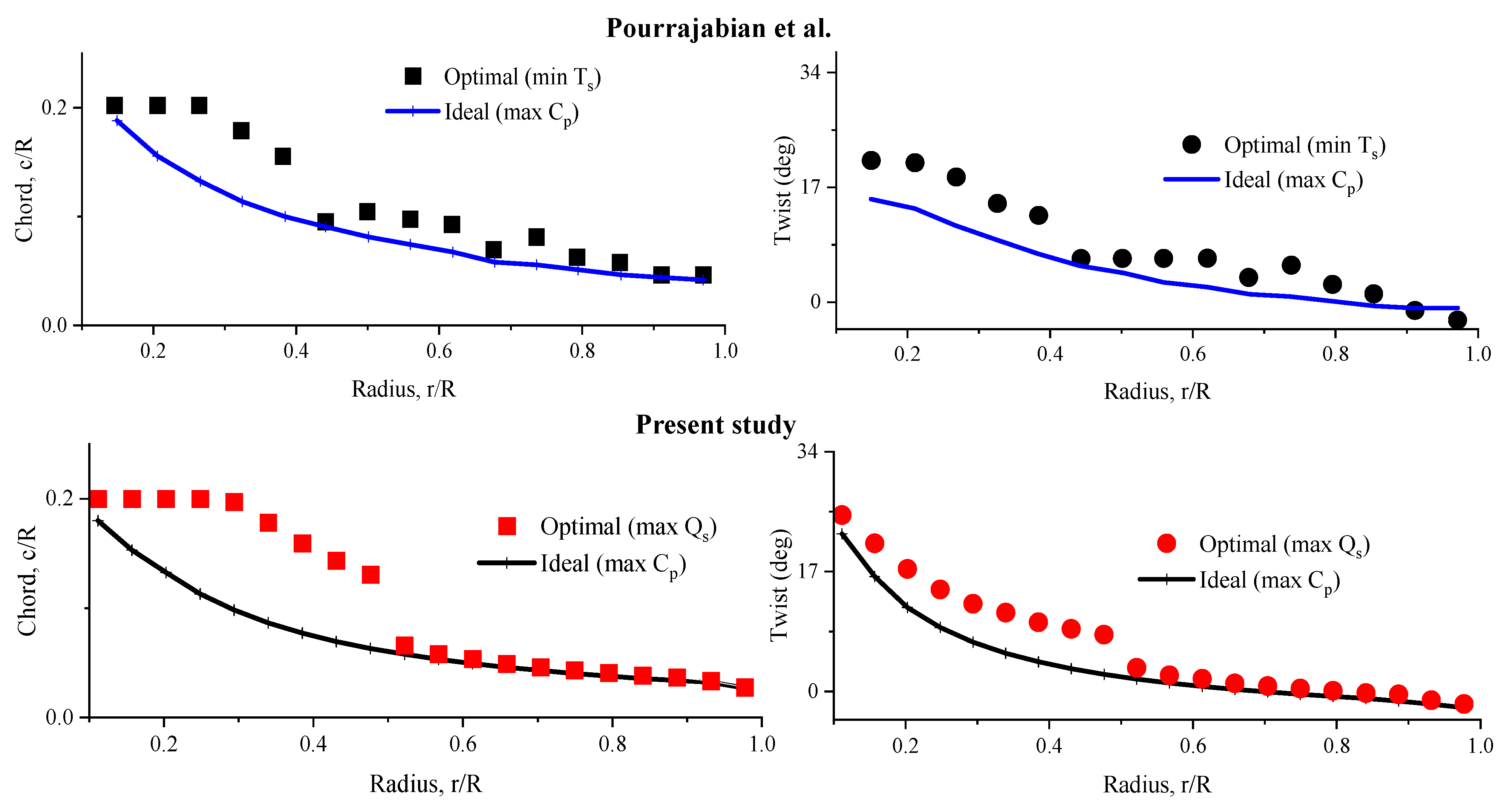
• In blade design, to obtain the maximum C_p, the genetic algorithm and the Schmitz equations reached a similar c and θ profiles, which indicates the high accuracy and capability of the genetic algorithm in optimizing wind turbine blades;
• The blade geometry designed with ideal equations produces the lowest Q_s, so these types of blades are not suitable for application in regions with low wind speed;
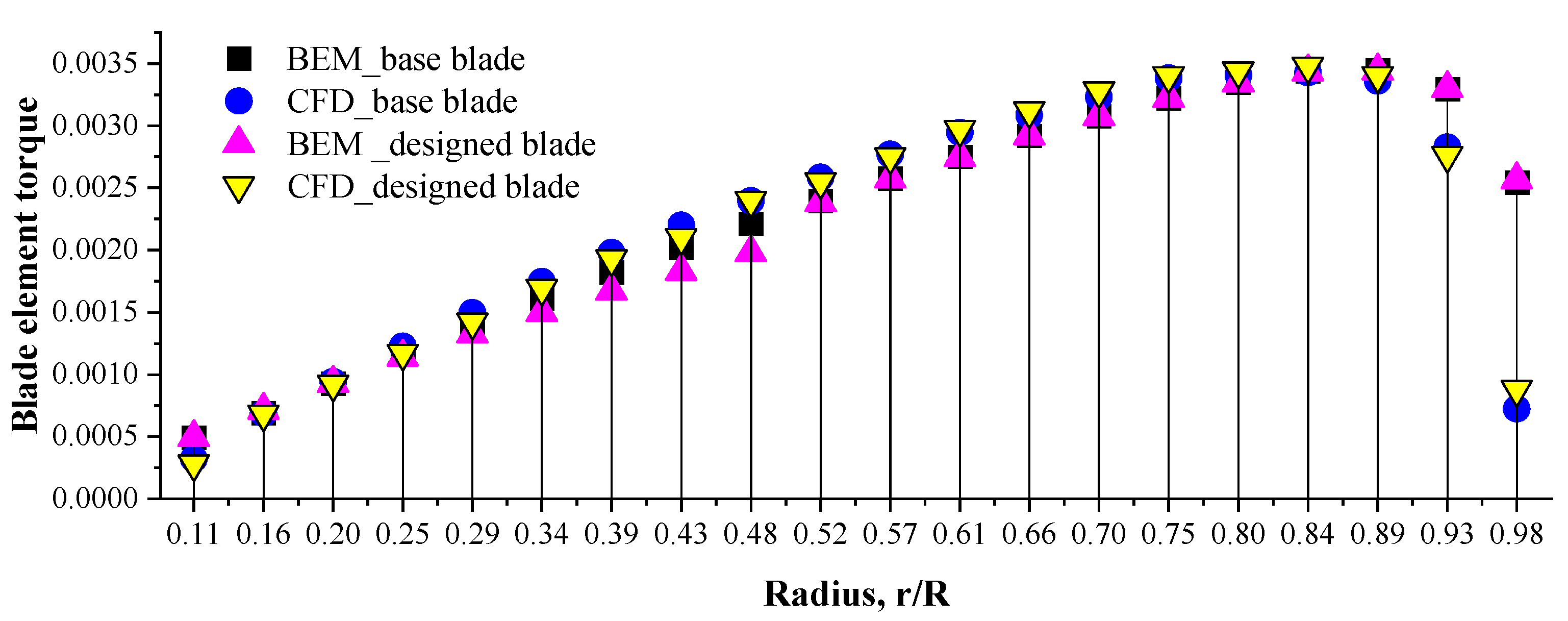
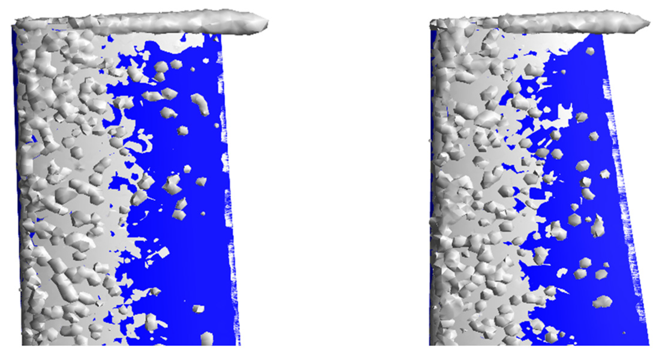
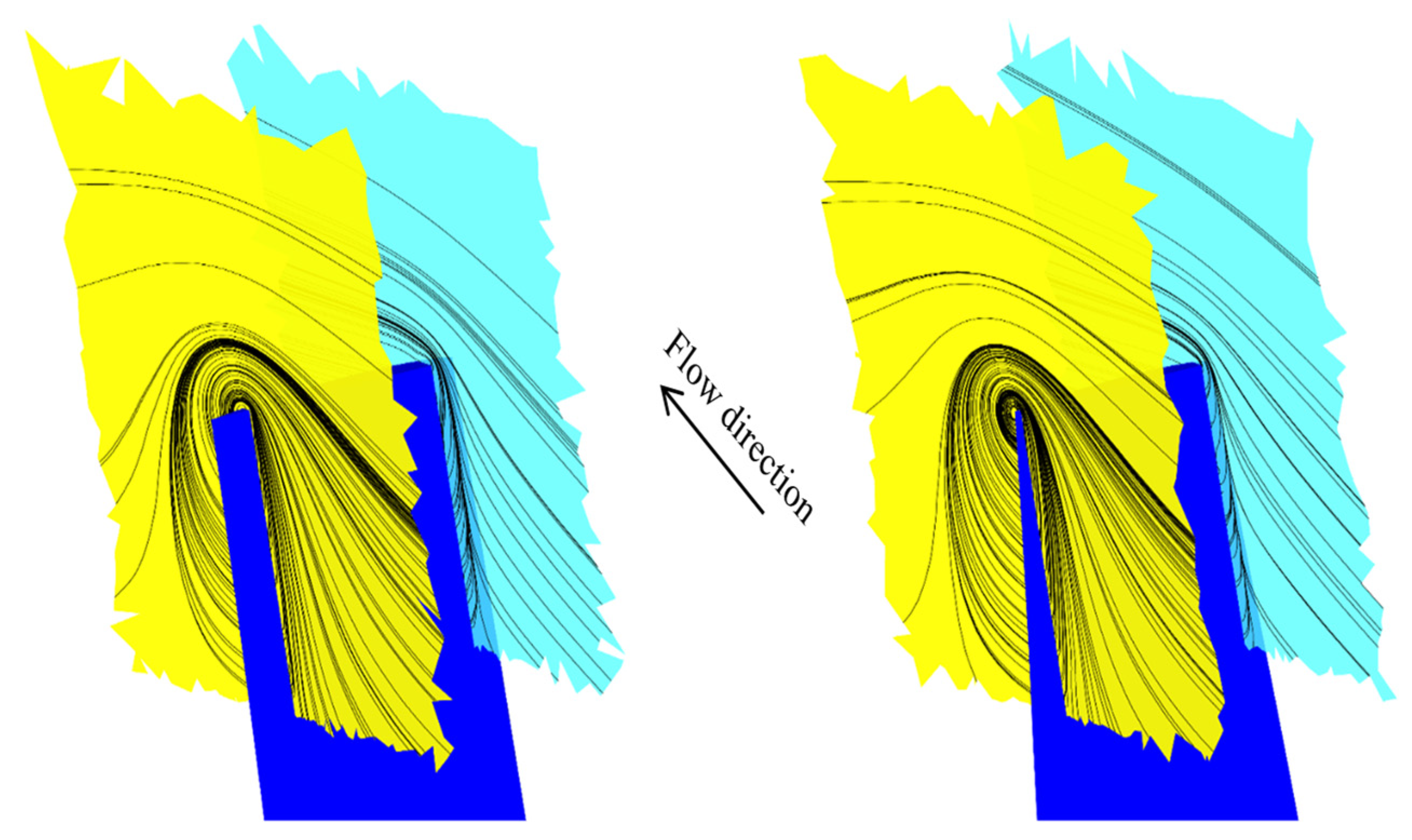
• The aerodynamic torque for power generation increases along the length of the blade from the hub to r/R = 0.89, and a good agreement can be seen between the CFD and BEM results up to this point, but after that, the aerodynamic torque decreases due to the formation of tip vortices. In this regard, the CFD method predicts a greater drop than Prandtl’s tip correction factor;
• Considering the Q_s in the objective function is very useful because, firstly, it leads to c and θ distributions without discrepancies, and, secondly, it results in a significant increase in the Q_s against a slight decrease in the output power. This compromise is very attractive for low-wind-speed areas;
• When the blade is stationary, the tip elements of the blade not only do not contribute to the Q_s but also can produce a negative torque which is due to the negative θ in this region.

References

1. United Nations. Transforming Our World: The 2030 Agenda for Sustainable Development; United Nations: New York, NY, USA, 2015.
2. Evans, A.; Strezov, V.; Evans, T.J. Assessment of Sustainability Indicators for Renewable Energy Technologies. Renew. Sustain. Energy Rev. 2009, 13, 1082–1088. [Google Scholar] [CrossRef]
3. Castellani, F.; Astolfi, D.; Becchetti, M.; Berno, F. Experimental and Numerical Analysis of the Dynamical Behavior of a Small Horizontal-Axis Wind Turbine under Unsteady Conditions: Part I. Machines 2018, 6, 52. [Google Scholar] [CrossRef]
4. Mostafaeipour, A. Economic Evaluation of Small Wind Turbine Utilization in Kerman, Iran. Energy Convers. Manag. 2013, 73, 214–225. [Google Scholar] [CrossRef]
5. Eltayesh, A.; Castellani, F.; Burlando, M.; Bassily Hanna, M.; Huzayyin, A.S.; El-Batsh, H.M.; Becchetti, M. Experimental and Numerical Investigation of the Effect of Blade Number on the Aerodynamic Performance of a Small-Scale Horizontal Axis Wind Turbine. Alex. Eng. J. 2021, 60, 3931–3944. [Google Scholar] [CrossRef]
6. Bourhis, M.; Pereira, M.; Ravelet, F. Experimental Investigation of the Effect of Blade Solidity on Micro-Scale and Low Tip-Speed Ratio Wind Turbines. 2022. Available online: https://papers.ssrn.com/sol3/papers.cfm?abstract_id=4049421 (accessed on 7 September 2022).
7. Wright, A.K.; Wood, D.H. The Starting and Low Wind Speed Behaviour of a Small Horizontal Axis Wind Turbine. J. Wind Eng. Ind. Aerodyn. 2004, 92, 1265–1279. [Google Scholar] [CrossRef]
8. Berges, B. Development of Small Wind Turbines; Technical University of Denmark: Lyngby, Denmark, 2007. [Google Scholar]
9. Hansen, M.O.L.; Aagaard Madsen, H. Review Paper on Wind Turbine Aerodynamics. J. Fluids Eng. Trans. ASME 2011, 133, 114001. [Google Scholar] [CrossRef]
10. Wood, D. Small Wind Turbines: Analysis, Design, and Application. In Green Energy and Technology; Springer: London, UK, 2011; Volume 38, ISBN 9781849961745. [Google Scholar]
11. Selig, M.S.; McGranahan, B.D. Wind Tunnel Aerodynamic Tests of Six Airfoils for Use on Small Wind Turbines. J. Sol. Energy Eng. 2004, 126, 986–1001. [Google Scholar] [CrossRef]
12. Singh, R.K.; Ahmed, M.R.; Zullah, M.A.; Lee, Y.H. Design of a Low Reynolds Number Airfoil for Small Horizontal Axis Wind Turbines. Renew. Energy 2012, 42, 66–76. [Google Scholar] [CrossRef]
13. Hassanzadeh, A.; Hassanabad, A.H.; Dadvand, A. Aerodynamic Shape Optimization and Analysis of Small Wind Turbine Blades Employing the Viterna Approach for Post-Stall Region. Alex. Eng. J. 2016, 55, 2035–2043. [Google Scholar] [CrossRef]
14. Burton, T.; Jenkins, N.; Sharpe, D.; Bossanyi, E. Wind Energy Handbook; John Wiley & Sons: Hoboken, NJ, USA, 2011; ISBN 111999392X. [Google Scholar]
15. Yang, X.S.; Deb, S. Cuckoo Search via Lévy Flights. In Proceedings of the 2009 World Congress on Nature & Biologically Inspired Computing (NaBIC 2009), Coimbatore, India, 9–11 December 2009; pp. 210–214. [Google Scholar] [CrossRef]
16. Garcia, F.J.M.; Pérez, J.A.M. Jumping Frogs Optimization: A New Swarm Method for Discrete Optimization. Doc. Trab. DEIOC 2008, 3, 1–10. [Google Scholar]
17. Yang, X.-S.S. A New Metaheuristic Bat-Inspired Algorithm BT—Nature Inspired Cooperative Strategies for Optimization (NICSO 2010). Stud. Comput. Intell. 2010, 284, 65–74. [Google Scholar]
18. Holland, J.H. Adaptation in Natural and Artificial Systems: An Introductory Analysis with Applications to Biology, Control, and Artificial Intelligence; MIT Press: Cambridge, MA, USA, 1992; ISBN 0262581116. [Google Scholar]
19. Dorigo, M.; Maniezzo, V.; Colorni, A. Ant System: Optimization by a Colony of Cooperating Agents. IEEE Trans. Syst. Man. Cybern. Part B Cybern. 1996, 26, 29–41. [Google Scholar] [CrossRef] [PubMed]
20. Engelbrecht, A.P. Fundamentals of Computational Swarm Intelligence; John Wiley & Sons: Hoboken, NJ, USA, 2005; Volume 599. [Google Scholar]
21. Soni, V.; Sharma, A.; Singh, V. A Critical Review on Nature Inspired Optimization Algorithms. IOP Conf. Ser. Mater. Sci. Eng. 2021, 1099, 012055. [Google Scholar] [CrossRef]
22. Pourrajabian, A. Effect of Blade Profile on the External/Internal Geometry of a Small Horizontal Axis Wind Turbine Solid/Hollow Blade. Sustain. Energy Technol. Assess. 2022, 51, 101918. [Google Scholar] [CrossRef]
23. Jureczko, M.; Mrówka, M. Multiobjective Optimization of Composite Wind Turbine Blade. Materials 2022, 15, 4649. [Google Scholar] [CrossRef]
24. Pourrajabian, A.; Dehghan, M.; Javed, A.; Wood, D. Choosing an Appropriate Timber for a Small Wind Turbine Blade: A Comparative Study. Renew. Sustain. Energy Rev. 2019, 100, 1–8. [Google Scholar] [CrossRef]
25. Akbari, V.; Naghashzadegan, M.; Kouhikamali, R.; Afsharpanah, F.; Yaïci, W. Multi-Objective Optimization and Optimal Airfoil Blade Selection for a Small Horizontal-Axis Wind Turbine (HAWT) for Application in Regions with Various Wind Potential. Machines 2022, 10, 687. [Google Scholar] [CrossRef]
26. Astolfi, D.; Castellani, F.; Natili, F. Wind Turbine Yaw Control Optimization and Its Impact on Performance. Machines 2019, 7, 41. [Google Scholar] [CrossRef]
27. Dal Monte, A.; Castelli, M.R.; Benini, E. Multi-Objective Structural Optimization of a HAWT Composite Blade. Compos. Struct. 2013, 106, 362–373. [Google Scholar] [CrossRef]
28. Clifton-Smith, M.J. Aerodynamic Noise Reduction for Small Wind Turbine Rotors. Wind Eng. 2010, 34, 403–420. [Google Scholar] [CrossRef]
29. Abdelsalam, A.M.; El-Askary, W.A.; Kotb, M.A.; Sakr, I.M. Experimental Study on Small Scale Horizontal Axis Wind Turbine of Analytically-Optimized Blade with Linearized Chord Twist Angle Profile. Energy 2021, 216, 119304. [Google Scholar] [CrossRef]
30. Rector, M.C.; Visser, K.D.; Humiston, C.J. Solidity, Blade Number, and Pitch Angle Effects on a One Kilowatt HAWT. In Proceedings of the Collection of Technical Papers—44th AIAA Aerospace Sciences Meeting, Reno, NV, USA, 9–12 January 2006; Volume 10, pp. 7281–7290. [Google Scholar]
31. Wang, S.-H.; Chen, S.-H. Blade Number Effect for a Ducted Wind Turbine. J. Mech. Sci. Technol. 2008, 22, 1984–1992. [Google Scholar] [CrossRef]
32. Astolfi, D.; Castellani, F.; Terzi, L. Wind Turbine Power Curve Upgrades. Energies 2018, 11, 1300. [Google Scholar] [CrossRef]
33. Anderson, M.B.; Milborrow, D.J.; Ross, J.N. Performance and Wake Measurements on a 3 M Diameter Horizontal Axis Wind Turbine. Comparison of Theory, Wind Tunnel and Field Test Data. In Proceedings of the International Symposium on Wind Energy Systems, Stockholm, Sweden, 21–24 September 1982; Volume 2, pp. 113–135. [Google Scholar]
34. Koca, K.; Genç, M.S.; Açıkel, H.H.; Çağdaş, M.; Bodur, T.M. Identification of Flow Phenomena over NACA 4412 Wind Turbine Airfoil at Low Reynolds Numbers and Role of Laminar Separation Bubble on Flow Evolution. Energy 2018, 144, 750–764. [Google Scholar] [CrossRef]
35. Glauert, H. Airplane Propellers. In Aerodynamic Theory; Springer: Berlin/Heidelberg, Germany, 1935; pp. 169–360. [Google Scholar]
36. Spera, D.A. Wind Turbine Technology; ASME Publishing: New York, NY, USA, 1994. [Google Scholar]
37. Castellani, F.; Astolfi, D.; Natili, F.; Mari, F. The Yawing Behavior of Horizontal-Axis Wind Turbines: A Numerical and Experimental Analysis. Machines 2019, 7, 15. [Google Scholar] [CrossRef]
38. Wood, D.H. A Blade Element Estimation of the Cut-in Wind Speed of a Small Turbine. Wind Eng. 2001, 25, 125–130. [Google Scholar] [CrossRef]
39. Holland, J. Adaptation in Natural and Artificial Systems; University of Michigan Press: Ann Arbor, MI, USA, 1975; Volume 7, pp. 390–401. [Google Scholar]
40. Goldberg, D.E. Genetic Algorithms; Pearson Education: Noida, India, 2013; ISBN 817758829X. [Google Scholar]
41. Haupt, R.L.; Haupt, S.E. Practical Genetic Algorithms; John Wiley & Sons: Hoboken, NJ, USA, 2004; ISBN 0471671754. [Google Scholar]
42. Gasch, R.; Twele, J. Blade Geometry According to Betz and Schmitz. In Wind Power Plants; Springer: Berlin/Heidelberg, Germany, 2012; pp. 168–207. [Google Scholar]
43. ANSYS Fluent Theory Guide; ANSYS, Inc.: Canonsburg, PA, USA, 2015.
44. Sessarego, M.; Wood, D. Multi-Dimensional Optimization of Small Wind Turbine Blades. Renew. Wind. Water Sol. 2015, 2, 9. [Google Scholar] [CrossRef] [Green Version]
Figure 1. Influential parameters in the shape of a wind turbine blade.
Machines 10 00785 g001
Figure 2. The geometry of the base turbine [33].
Machines 10 00785 g002
Figure 3. The geometry of the NACA4412 airfoil.
Machines 10 00785 g003
Figure 4. Flowchart of the optimization process.
Machines 10 00785 g004
Figure 5. The variations in the drag and lift coefficients of the NACA4412 profile [10].
Machines 10 00785 g005
Figure 6. The changes of C P at various λ for the current research and the study of Anderson et al. [33].
Machines 10 00785 g006
Figure 7. The distributions of θ (top) and c (bottom) obtained from the optimization algorithm and ideal correlations.
Machines 10 00785 g007
Figure 8. The Pareto front for the optimized blades.
Machines 10 00785 g008
Figure 9. The θ and c profiles for the blades with different n values.
Machines 10 00785 g009
Figure 10. The θ and c profiles of the optimal blade in the research of Pourrajabian et al. [24] and the optimal blade of the present study.
Machines 10 00785 g010
Figure 11. The geometry of the base (a) and designed (b) blades.
Machines 10 00785 g011
Figure 12. The computational domain and boundary conditions.
Machines 10 00785 g012
Figure 13. The generated mesh for the computational domain.
Machines 10 00785 g013
Figure 14. The y + distribution contours on the suction sides of the blades.
Machines 10 00785 g014
Figure 15. The grid-independency test results.
Machines 10 00785 g015
Figure 16. The generated aerodynamic torque along the blade during power generation.
Machines 10 00785 g016
Figure 17. The tip vortices of the base (left) and designed (right) blades.
Machines 10 00785 g017
Figure 18. The tip streamlines of the base (left) and designed (right) blades.
Machines 10 00785 g018
Figure 19. The Qs values generated by the base/designed blades.
Machines 10 00785 g019
Figure 20. The Qs generated in each element.
Machines 10 00785 g020
Figure 21. Changes of λ during the startup process for the designed and base blades.
Machines 10 00785 g021
Figure 22. Variations of the Qs up to λ = 2 for the designed and base blades.
Machines 10 00785 g022