Adaptive Neural-PID Visual Servoing Tracking Control via Extreme Learning Machine

Abstract

The vision-guided robot is intensively embedded in modern industry, but it is still a challenge to track moving objects in real time accurately. In this paper, a hybrid adaptive control scheme combined with an Extreme Learning Machine (ELM) and proportional–integral–derivative (PID) is proposed for dynamic visual tracking of the manipulator. The scheme extracts line features on the image plane based on a laser-camera system and determines an optimal control input to guide the robot, so that the image features are aligned with their desired positions. The observation and state–space equations are first determined by analyzing the motion features of the camera and the object. The system is then represented as an autoregressive moving average with extra input (ARMAX) and a valid estimation model. The adaptive predictor estimates online the relevant 3D parameters between the camera and the object, which are subsequently used to calculate the system sensitivity of the neural network. The ELM–PID controller is designed for adaptive adjustment of control parameters, and the scheme was validated on a physical robot platform. The experimental results showed that the proposed method’s vision-tracking control displayed superior performance to pure P and PID controllers.

1. Introduction

Robotic vision has important commercial and domestic applications such as in assembly and welding, fruit picking, and household services. Most robots, however, follow a set program to complete repetitive tasks. When discrepancies occur in the target or the robot, it tends to be unable to make timely environmental adjustments, which is largely due to the inherent lack of an adequate perception capability [1]. Visual servoing enables dexterous control of robots through continuous visual perception and has drawn consistent attention.

Since 1996, Hutchinson’s three classic surveys [2,3,4] have provided a systematic understanding of visual servoing. According to the representation of control signals, it can be categorized as position-based (PBVS), image-based (IBVS) or hybrid (HVS). In particular, IBVS has attracted widespread interest for its simple structure and insensitivity to calibration accuracy. Common methods of IBVS control are adaptive [5], sliding mode [6], fuzzy [7] and learning-based [8]. Saleem et al. [9] proposed an adaptive fuzzy-tuned proportional derivative (AFT-PD) control scheme to improve the visual tracking control of a mobile wheeled robot. YANG et al. [10] used radial basis function (RBF) neural networks to estimate the dynamic parameters of the robot and compensate for the robot’s torque to improve the tracking performance of the controller.

Most IBVS studies have been carried out under the assumption that the target is stationary, so visual tracking in dynamic scenes has rarely been considered. Certain researchers have estimated the Jacobi matrix of IBVS by developing an adaptive algorithm. Chang [11] and Gongye [12] proposed Kalman filtering to provide the unknown depth information of the image Jacobi matrix in real time and verified its practicality on a manipulator. Music [13] established particle filtering and the Broyden algorithm to estimate the Jacobian matrix. Simulation experiments were performed to compare the trajectory tracking performance in static and dynamic scenes. The results showed that the Broyden computation time was much less than that of particle filtering, but its performance was vulnerable to noise interference.

In recent work, learning-based IBVS control has been used to optimize the parameters or to construct nonlinear estimators [14,15]. RBF neural networks combined with PI controllers were used to improve the accuracy of trajectory tracking of a dual robotic arm [16]. From a different perspective, the RBF is used as the inverse kinematics solver of the robotic arm, which was obtained by training the samples of the forward kinematics. The results showed that the method effectively improves the positioning accuracy of visual servoing [17]. To address the low stability of the visual servoing, Shi [18] proposed using Q-learning to adjust the control parameters of visual servoing adaptively, and to optimize the parameters of Q-learning further using a fuzzy-based method to improve the convergence and the stability of the control system. Overall, the above works have proved the effectiveness of the method only in static scenarios. Indeed, the dynamic convergence and responsiveness have not been adequately analyzed.

The image feature extraction is also an essential aspect that affects the reliability behavior of the control system. In visual servoing, the system needs to extract valid features in the image sequence and drive the robot motion while minimizing errors between the current and the reference image. Therefore, the representation of the image Jacobi matrix, i.e., the velocity variation relationship between the target in image space and in Cartesian space, is an essential part of vision tracking. The point features [19], optical flow [20] and image moments [21] have been extensively studied in visual tracking. However, the reliability problem of feature matching in complex scenes has not been well addressed. To ameliorate that, direct visual servoing (DVS) has been proposed in recent years [22,23,24].

Instead of the common local image feature extraction techniques, DVS uses the whole image to construct a mapping relationship with the robot’s joint pose, which is obtained by acquiring a large amount of data, (usually several thousand samples) and feeding it into a neural network. Although DVS enhances the robustness of feature extraction and significantly reduces the time spent on image processing, the acquisition of its samples and the training process are time-consuming. Additionally, the network needs to be retrained when the environment changes, which greatly diminishes its practical feasibility.

As mentioned, in previous research findings, the primary limitation of the robot’s visual servoing dynamic tracking performance is the estimation speed and accuracy of the image Jacobi matrix, and the design of the controller [25]. Therefore, our work in this paper is focused on the above-mentioned bottlenecks. In the hardware system, a laser-camera vision system implements the acquisition of image information. The system consists of a camera rigidly mounted on the robot end-effector, and a laser stripe generator. The camera is used to acquire image information and the laser stripe generator is used to project visible light onto the table. The inertial principal axis of the target is recognized and used as desired image features, while the visible straight line on the plane is used as the current image feature. Hence, in this paper the visual tracking problem was transformed into an error minimization problem of line feature, the inimitable strengths of which have been proven in welding robots and bricklaying robots [26,27].

This research is concerned with implementing line feature visual servoing. This work was conducted within the framework of a robotic bricklaying project. The main partner was a construction company in Guangxi Province, and the primary concerns were to automate the robot’s masonry work, particularly precise brick placement, since relatively large operating errors may adversely affect the strength of the building. Cutting-edge masonry robots still require strict calibration of the hand-eye and working environment, which may lead to deteriorating operational effectiveness if unexpected deviations of the robot’s position occur. Thus, it is necessary to use the sensing technology with closed-loop control, such as visual servoing. Since manual masonry typically uses laser lines for alignment and the bricks are composed of three intersecting orthogonal planes from which points features may not be reliably extracted, we focused our research on enabling visual servoing based on line features.

For the design of the controller, a hybrid ELM–PID control scheme was proposed for real-time visual tracking by a six-degree-of-freedom robot. We gave the observation and the state-space equations by analyzing the motion rules of the camera and the object. The system was then represented as a time-varying multi-input/multi-output autoregressive moving average model. Subsequently, an ELM model was proposed to predict the relevant Jacobian information, which uses the measured data of the previous moment as an input to predict the result of the next moment. These prediction parameters were then used as the online input of the gradient descent algorithm. To perform faster adaptive tuning of the controller parameters, a three-layer structured BP neural network was used. The aim of this study was to perform an algorithm-level validation of robotic autonomous masonry and to further assess the positioning accuracy and control speed in static and dynamic environments.

This paper is organized as follows: Section 2 presents visual tracking modeling. In Section 3, we introduce the adaptive estimation of visual tracking. Section 4 analyzes the ELM–PID controller implementation. Section 5 shows the experimental design, and Section 6 analyzes the experimental results. Finally, conclusions are drawn in Section 7.

2. Visual Tracking Modeling

2.1. Camera Model and Feature Motion

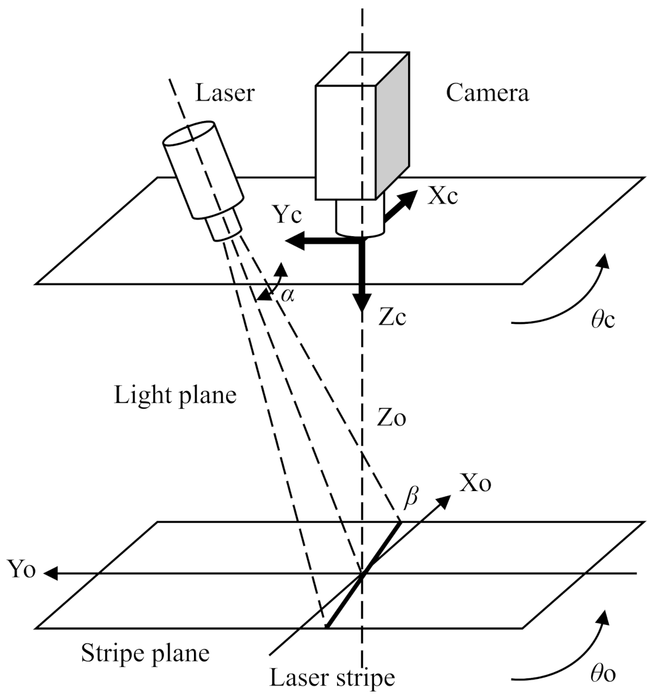
Visual tracking is implemented by a laser-camera system consisting of a camera mounted on the end-effector to acquire image information and guide the robot’s movement, as shown in Figure 1. The vision-tracking task in this paper was to align the laser streak line with the principal axis of inertia of the target image. A laser streak is visible light projected onto a plane by a laser sensor. The principal axis of inertia can be obtained by simple image processing. We define the camera’s focal point as the origin of the image plane. Assuming a perspective projection and the focal length to be unity, a point $\mathbf{P}=(X,Y,Z)$ in the camera frame projects onto a $\mathbf{p}=(x,y)$ in the image coordinates such that

$$x=\frac{X}{Z},y=\frac{Y}{Z}$$

(1)

Taking the temporal derivative of the projection in Equation (1), we obtain

$$\left\{\begin{array}{c}\dot{x}=\frac{\dot{X}Z-X\dot{Y}}{Z^2}\hfill \\ \dot{y}=\frac{\dot{Y}Z-Y\dot{Z}}{Z^2}\hfill \end{array}\right.$$

(2)

Consider a camera moving with a body velocity $v=(T,w)$ in the world frame and observing a world point $\mathbf{p}$ with camera-relative coordinates $\mathbf{P}=(X,Y,Z)$. Assume that the camera moves with a transnational velocity $\mathbf{T}=(T_X,T_Y,T_Z)$ and a rotational velocity $\mathrm{\Omega }=({\mathrm{\Omega }}_X,{\mathrm{\Omega }}_Y,{\mathrm{\Omega }}_Z)$. The velocity of the point relative to the camera frame is

$$\dot{\mathbf{P}}=-T\times \mathbf{P}-\mathrm{\Omega }$$

(3)

which we can write in scalar form as

$$\left\{\begin{array}{c}\dot{X}=-T_x-{\mathrm{\Omega }}_{y}Z+{\mathrm{\Omega }}_{z}Y\hfill \\ \dot{Y}=-T_y-{\mathrm{\Omega }}_{z}X+{\mathrm{\Omega }}_{x}Z\hfill \\ \dot{Z}=-T_z-{\mathrm{\Omega }}_{x}Y+{\mathrm{\Omega }}_{y}X\hfill \end{array}\right.$$

(4)

From combining Equations (2) and (4), and grouping terms we obtain

$$\left\{\begin{array}{c}\dot{x}=x\frac{T_Z}{Z}-\frac{T_X}{Z}+xy{\mathrm{\Omega }}_X-\left(1+x^2\right){\mathrm{\Omega }}_Y+y{\mathrm{\Omega }}_Z\hfill \\ \\ \dot{y}=y\frac{T_Z}{Z}-\frac{T_Y}{Z}+\left(1+y^2\right){\mathrm{\Omega }}_X-xy{\mathrm{\Omega }}_Y-x{\mathrm{\Omega }}_Z\hfill \end{array}\right.$$

(5)

Equation (5) defines the image Jacobi of the point features, which describe the velocity transformation between the spatial motion of the camera and the image feature points. Consider the visible light line as the laser beam’s projection on the image plane. The equation of the line on the image is expressed as follows

$$\rho =xcos\theta +ysin\theta$$

(6)

where $\rho$ is the signed vertical distance of the line to the origin, and $\theta$ is the angle of the line with respect to the x-axis. The coordinates of the points on the line are denoted as x and y. The velocity relationship of line feature can be given as

$$\left\{\begin{array}{c}\dot{\theta }={\lambda }_{\theta }cos\theta T_X+{\lambda }_{\theta }sin\theta T_Y-{\lambda }_{\theta }\rho T_Z-\rho cos\theta {\mathrm{\Omega }}_X-\rho sin\theta {\mathrm{\Omega }}_Y-{\mathrm{\Omega }}_Z\hfill \\ \dot{\rho }={\lambda }_{\rho }cos\theta T_X+{\lambda }_{\rho }sin\theta T_Y-{\lambda }_v\rho T_Z+{(1+\rho )}^{2}sin\theta {\mathrm{\Omega }}_X-{(1+\rho )}^{2}cos\theta {\mathrm{\Omega }}_Y\hfill \end{array}\right.$$

(7)

where ${\lambda }_{\theta }=(a_{i}sin\theta -b_{i}cos\theta )/d_i$, and ${\lambda }_{\rho }=(a_i\rho cos\theta +b_i\rho sin\theta +c_i)/d_i$. The parameters of $a_i$, $b_i$, $c_i$ and $d_i$ are the normal vectors of the polyhedral plane.

To convert from two-dimensional image coordinates to three-dimensional spatial coordinates, the system shown in Figure 1 must be calibrated accurately. In the process, the values of the disparity angle $\alpha$, the tilt angle $\beta$, and the offset $Y_o$ will be determined.

2.2. Observation Equation

Considering that quite a large part of the research has explored the use of lines in visual servoing by pegging out constant depth information (e.g., automated welding, lane keeping for autonomous driving), we simplified the problem to a set of assumptions. Suppose the object is moving in plane $P_A$ and the camera and laser stripe sensor are moving in plane $P_B$. Here, the two planes are parallel to each other, and the distance between them ($Z_o$) is constant. The z-axis of the camera is perpendicular to these two planes. Consider a coordinate point p, the intersection of a straight line and its perpendicular line through the origin. In the image space, the laser-stripe lines will be aligned with the minimum inertia principal axis of the object. The observation equations can be given as

$$\mathbf{x}:={(\rho cos\theta ,\rho sin\theta ,\theta -\frac{\pi }{2})}^T$$

(8)

$$\mathbf{y}:={(x,y,\omega )}^T$$

(9)

$$\mathbf{w}:={\left(w_x,w_y,w_{\omega }\right)}^T$$

(10)

$$\mathbf{y}=\mathbf{Cx}+\mathbf{w}$$

(11)

where $\omega$ is the tangent angle of the line; $\mathbf{C}={\mathbf{I}}_3$; and $\mathbf{w}$ is an observation noise vector. The measurement vector is acquired in a manner slightly different from the method used to track individual feature points.

2.3. State–Space Equation

Define each time $t=k{T}_s,k=1,2,3,\dots$, where $Ts$ denotes the sampling period, so that the observation Equation (11) becomes

$$\mathbf{y}\left(k\right)=\mathbf{C}\mathbf{x}\left(k\right)+\mathbf{w}\left(k\right)$$

(12)

The output vector $\mathbf{y}\left(k\right)$ can be obtained directly as the output of the vision. The state variables $\mathbf{x}\left(k\right)$ can be obtained if the white noise terms $\mathbf{w}\left(k\right)$ are ignored due to uncertainties.

$$T_{cZ}=T_{oZ}={\mathrm{\Omega }}_{cX}={\mathrm{\Omega }}_{cY}={\mathrm{\Omega }}_{oX}={\mathrm{\Omega }}_{oY}=0$$

(13)

To construct the state equation to describe the system dynamics, the velocities of the camera were defined as $(T_{cX},T_{cY},T_{cZ})$ and $({\mathrm{\Omega }}_{cX},{\mathrm{\Omega }}_{cY},{\mathrm{\Omega }}_{cZ})$, and the velocities of the object feature were denoted as $(T_{oX},T_{oY},T_{oZ})$ and $({\mathrm{\Omega }}_{oX},{\mathrm{\Omega }}_{oY},{\mathrm{\Omega }}_{oZ})$. Combining Equations (4)–(7) and (13), we have

$$U_c={\dot{x}}_c=cos\theta \dot{\rho }-\rho sin\theta \dot{\theta }=\left({\lambda }_{\rho }{cos}^2\theta -{\lambda }_{\theta }\rho sin\theta cos\theta \right)T_{cx}$$

(14)

$$V_c={\dot{y}}_c=sin\theta \dot{\rho }+\rho cos\theta \dot{\theta }=\left({\lambda }_{\rho }{sin}^2\theta +{\lambda }_{\theta }\rho sin\theta cos\theta \right)T_{cY}$$

(15)

$${\mathrm{\Theta }}_c={\dot{\omega }}_c=-{\mathrm{\Omega }}_{cZ}$$

(16)

$$U_o={\dot{x}}_o=-\frac{1}{Z_0}{T}_{ox}$$

(17)

$$V_o={\dot{y}}_o=-\frac{1}{Z_0}{T}_{oY}$$

(18)

$${\mathrm{\Theta }}_o={\dot{\omega }}_o=\left(y_o-x_o\right){\mathrm{\Omega }}_{oZ}$$

(19)

where $U_c$, $V_c$ and ${\mathrm{\Theta }}_c$ are the components of the tracking motion of the camera. $U_o$, $V_o$ and ${\mathrm{\Theta }}_o$ are the components of the tracking motion of the object. If the optical flow of the point $\mathbf{p}$ at moment k is $(U_k,V_k,{\mathrm{\Theta }}_k)$, its optical flow can be expressed as

$$U\left(k\right)=U_c\left(k\right)+U_o\left(k\right)=S_{cU}\left(k\right)T_{cX}\left(k\right)+S_{oU}\left(k\right)T_{oX}\left(k\right)$$

(20)

$$V\left(k\right)=V_c\left(k\right)+V_o\left(k\right)=S_{cV}\left(k\right)T_{cY}\left(k\right)+S_{oV}\left(k\right)T_{oY}\left(k\right)$$

(21)

$$\mathrm{\Theta }\left(k\right)={\mathrm{\Theta }}_c\left(k\right)+{\mathrm{\Theta }}_o\left(k\right)=S_{c\mathrm{\Theta }}\left(k\right){\mathrm{\Omega }}_{cZ}\left(k\right)+S_{o\mathrm{\Theta }}\left(k\right){\mathrm{\Omega }}_{oZ}\left(k\right)$$

(22)

where

$$S_{cU}\left(k\right)={\lambda }_{\rho }{cos}^2\theta -{\lambda }_{\theta }\rho sin\theta cos\theta$$

(23)

$$S_{cV}\left(k\right)={\lambda }_{\rho }{sin}^2\theta +{\lambda }_{\theta }\rho sin\theta cos\theta$$

(24)

$$S_{c\mathrm{\Theta }}\left(k\right)=-1,S_{oU}\left(k\right)=-\frac{1}{Z_0}$$

(25)

$$S_{oV}\left(k\right)=-\frac{1}{Z_0},S_{o\mathrm{\Theta }}\left(k\right)=y-x$$

(26)

By applying $U\left(k\right)=(x(k+1)-x\left(k\right))/T_s$; $V\left(k\right)=(y(k+1)-y\left(k\right))/T_s$, and $\mathrm{\Theta }\left(k\right)=(\omega (k+1)-\omega \left(k\right))/T_s$; and Equations (14)–(22) the state–space representation can be given as

$$\mathbf{x}(k+1)=\mathbf{A}\mathbf{x}\left(k\right)+\mathbf{Bu}\left(k\right)+\mathbf{D}\tau \left(k\right)$$

(27)

where $\mathbf{x}(k)=(x(k),y(k);{\omega (k))}^T\in R^3$ is the state vector; $\mathbf{u}\left(k\right)=(T_{cX}\left(k\right),T_{cY}\left(k\right),{\mathrm{\Omega }}_{cZ}{\left(k\right))}^T\in R^3$ is the input vector; and $\tau \left(k\right)=(T_{oX}\left(k\right),T_{oY}\left(k\right),{\mathrm{\Omega }}_{oZ}{\left(k\right))}^T\in R^3$ is the exogenous disturbances vector or the state-noise vector. $x\left(k\right)$, $y\left(k\right)$, and $\omega \left(k\right)$ are now the tracking errors respectively. The matrixes $\mathbf{A}$, $\mathbf{B}$ and $\mathbf{D}$ are given as

$$\mathbf{B}=T_s\left(\begin{array}{ccc}{\lambda }_{\rho }{cos}^2\theta -{\lambda }_{\theta }\rho sin\theta cos\theta & 0& 0\\ 0& {\lambda }_{\rho }{sin}^2\theta +{\lambda }_{\theta }\rho sin\theta cos\theta & 0\\ 0& 0& -1\end{array}\right)$$

(28)

$$\mathbf{D}=T_s\left(\begin{array}{ccc}-\frac{1}{Z_0}& 0& 0\\ 0& -\frac{1}{Z_0}& 0\\ 0& 0& y-x\end{array}\right),\mathrm{and}\mathbf{A}={\mathbf{I}}_3$$

(29)

Considering the scenarios where the depth information changes (e.g., robot grasping), Equations (13)–(29) will be modified acordingly. Evidently, the above changes do not affect any of the inference results after Section 2, so the proposed method is still valid outside the assumed constraints.

3. Adaptive Estimation of Visual Tracking

3.1. Adaptive Estimation Model

Dynamic parameters (i.e., relative poses between the camera and the object) are necessary for visual servoing. When they are known, the Kalman filter method can be used to control the system. However, in a practical scene, the dynamics of the camera and the object may be unknown. Adaptive control techniques can be used as an alternative method. Equation (27) can be expressed as the last n states and control inputs such that

$$\mathbf{x}(k+n)={\mathbf{A}}^n\mathbf{x}\left(k\right)+\sum _{i=1}^n{\mathbf{A}}^{i-1}[\mathbf{B}\mathbf{u}(k+n-i)+\mathbf{D}\tau (k+n-i)]$$

(30)

Suppose $\mathbf{A}$ is a characteristic polynomial such that

$$f\left(\lambda \right)={\lambda }^n+a_1{\lambda }^{n-1}+\cdots +a_n,n=3$$

(31)

and by applying the Cayley–Hamilton theorem, we can obtain

$$\begin{array}{cc}\hfill \mathbf{y}(k+n)=& -\sum _{j=1}^n{a}_j\mathbf{y}(k+n-j)+\sum _{j=1}^{n-1}{a}_{n-j}\sum _{i=1}^j\mathbf{C}{\mathbf{A}}^{i-1}\mathbf{B}\mathbf{u}(k+j-i)\hfill \\ \hfill & +\sum _{i=1}^n\mathbf{C}{\mathbf{A}}^{i-1}\mathbf{B}\mathbf{u}(k+n-i)+\sum _{j=1}^{n-1}{a}_{n-j}\sum _{i=1}^j\mathbf{C}{\mathbf{A}}^{i-1}\mathbf{D}\tau (k+j-i)\hfill \\ \hfill & +\sum _{i=1}^n\mathbf{C}{\mathbf{A}}^{i-1}\mathbf{D}\tau (k+n-i)+\sum _{i=1}^n{a}_j\mathbf{w}(k+n-j)+\mathbf{w}(k+n)\hfill \end{array}$$

(32)

According to the ARMAX model, the previous system can be written as

$$A\left(z^{-1}\right)y\left(k\right)=z^{-d}\left[B_{ij}\left(z^{-1}\right)\right]u\left(k\right)+\left[C_{ij}\left(z^{-1}\right)\right]\eta \left(k\right)$$

(33)

where

$$A\left(z^{-1}\right)=1+a_1{z}^{-1}+a_2{z}^{-2}+\cdots +a_n{z}^{-n}$$

(34)

$$B_{ij}\left(z^{-1}\right)=b_1^{ij}{z}^{-1}+b_2^{ij}{z}^{-2}+\cdots +b_n^{ij}{z}^{-n}$$

(35)

$$C_{ij}\left(z^{-1}\right)=c_1^{ij}{z}^{-1}+c_2^{ij}{z}^{-2}+\cdots +c_n^{ij}{z}^{-n}$$

(36)

where $n=3$ is the dimension of the vector; $\mathbf{y}\left(k\right)$ and $\mathbf{u}\left(k\right)$ are the n-dimensional output and input, respectively; $\eta \left(k\right)$ is the n-dimensional noise term that is a combination of the state noise $\tau \left(k\right)$ and the observation noise $w\left(k\right)$; and $z^{-1}$ is the unit delay operator. Since the image processing requires a finite time, d is defined as a delay factor with a value of 1. $A\left(z^{-1}\right)$ is a scalar polynomial in $z^{-1}$. $\left[B_{ij}{z}^{-1}\right]$ and $\left[C_{ij}{z}^{-1}\right]$ are the scalar polynomial matrices of $B_{ij}{z}^{-1}$ and $C_{ij}{z}^{-1}$, respectively. Moreover, $\eta \left(k\right)$ is a sequence of independent equidistributed Gaussian variables with 0 mean and ${\delta }^2$ variance.

3.2. Estimation Schemes

The unknown parameters of the system can be estimated by the least squares method. The predictor gives the optimal prediction based on the historical measurements. Equation (33) can be expressed in the form of an optimal predictor (d = 1) such that

$$c^{opt}\left(z^{-1}\right)y^{opt}(k+d\mid k)=\left[A_{ij}^{opt}\left(z^{-1}\right)\right]y\left(k\right)+\left[B_{ij}^{opt}\left(z^{-1}\right)\right]u\left(k\right)$$

(37)

where

$$c^{opt}\left(z^{-1}\right)=det\left[C_{ij}\left(z^{-1}\right)\right]$$

(38)

$$\left.y^{opt}(k+d\mid k)=\left\{y(k+d)-\left[F_{ij}\left(z^{-1}\right)\right]\eta (k+d)\right]\right\}$$

(39)

$$\left[A_{ij}^{opt}\left(z^{-1}\right)\right]=\left[G_{ij}\left(z^{-1}\right)\right]\left[{\Re }_{ij}\left(z^{-1}\right)\right]$$

(40)

$$\left[B_{ij}^{opt}\left(z^{-1}\right)\right]=\left[F_{ij}\left(z^{-1}\right)\right]\left[{\Re }_{ij}\left(z^{-1}\right)\right]\left[B_{ij}\left(z^{-1}\right)\right]$$

(41)

$$\left[{\mathfrak{R}}_{ij}\left(z^{-1}\right)\right]=Adj\left[C_{ij}\left(z^{-1}\right)\right]$$

(42)

where the $F\left(z^{-1}\right)$ and $G\left(z^{-1}\right)$ are obtained by using the division algorithm, and $C\left(z^{-1}\right)=F\left(z^{-1}\right)A\left(z^{-1}\right)+z^{-\mathrm{d}}G\left(z^{-1}\right)$, respectively. The term $y^{opt}(k+d\mid k)$ denotes the optimal output prediction, and the term $y\left(k\right)$ denotes the output of the adaptive predictor.

If $\left[A_i^{opt}\left(z^{-1}\right)\right]$ is denoted as the ith row of both $\left[A_{ij}^{opt}\left(z^{-1}\right)\right]$ and $\left[B_i^{opt}\left(z^{-1}\right)\right]$, we have

$$c^{opt}\left(z^{-1}\right)\left(y_i^{opt}(k+d\mid k)-y_i^{*}(k+d)\right)=\left[A_i^{opt}\left(z^{-1}\right)\right]y\left(k\right)+\left[B_i^{opt}\left(z^{-1}\right)\right]u\left(k\right)-c^{opt}\left(z^{-1}\right)y_i^{*}(k+d)$$

(43)

If the polynomials $c^{opt}\left(z^{-1}\right)$ have some of their zeros on the unit circle, a predictor with sub-optimal performance can be designed. ${\mathbf{y}}_i^{*}(k+1)$ is given by

$${\mathbf{y}}_i^{*}(k+1)={\Delta }_i^T\left(k\right){\widehat{\mathrm{\Phi }}}_i\left(k\right)$$

(44)

where

$${\Delta }_i^T\left(k\right)=\left(y\left(k\right),y(k-1),\cdots ,u_i\left(k\right),u_i(k-1),\cdots ,-y_i^{*}\left(k\right),-y_i^{*}(k-1),\cdots \right)$$

(45)

$${\widehat{\mathrm{\Phi }}}_i\left(k\right)=\left({\widehat{a}}_{i1}\left(k\right),{\widehat{a}}_{i2}\left(k\right),\cdots ,{\widehat{b}}_{i1}\left(k\right),{\widehat{b}}_{i2}\left(k\right),\cdots ,{\widehat{c}}_{i1}\left(k\right),{\widehat{c}}_{i2}\left(k\right),\cdots \right)$$

(46)

Due to the time-varying nature of the estimated parameters, the well-known least square error method is used to estimate the unknown values of the parameters and can be estimated on-line by

$${\widehat{\mathrm{\Phi }}}_i(k+1)={\widehat{\mathrm{\Phi }}}_i\left(k\right)+{\mathsf{\Gamma }}_i\left(k\right){\Delta }_i\left(k\right)e_i(k+1)$$

(47)

$${\mathsf{\Gamma }}_i\left(k\right)=\frac{1}{{\mu }_i}\left[{\mathsf{\Gamma }}_i(k-1)-\frac{{\mathsf{\Gamma }}_i(k-1){\Delta }_i\left(k\right){\Delta }_i^T\left(k\right){\mathsf{\Gamma }}_i(k-1)}{{\mu }_i+{\Delta }_i^T\left(k\right){\mathsf{\Gamma }}_i(k-1){\Delta }_i\left(k\right)}\right]$$

(48)

$$e_i(k+1)=y_i(k+1)-y_i^{*}(k+1)$$

(49)

where the superscript i refers to the object model; the caret indicates the estimated value; ${\mu }_i\in (0,1]$ is a forgetting factor used to discount an exponential decay of the past data. ${\mathsf{\Gamma }}_i\left(k\right)$ is a covariance matrix.

4. ELM–PID Control Algorithm for Visual Servo

4.1. Extreme Learning Machine

ELM is a single hidden layer feedforward neural network proposed by Huang [28]. It differs significantly from the traditional feedforward neural network by using a gradient descent algorithm in the training phase. The weights and biases between the input and hidden layers of the network are set randomly and not adjusted after setting. Instead of iterative adjustment, the weights $\mathbf{\beta }$ between the hidden and output layers are determined by solving the generalized inverse matrix. Compared with traditional back-propagation learning algorithms, ELM has better training speed and generalization performance [29,30]. For N arbitrary samples $({\mathbf{X}}_i,{\mathbf{t}}_i)$, where ${\mathbf{X}}_i={\left[x_{i1},x_{i2},\cdots ,x_{in}\right]}^T\in {\mathbf{R}}^n$; and ${\mathbf{t}}_i={\left[t_{i1},t_{i2},\cdots ,t_{im}\right]}^T\in {\mathbf{R}}^m$. The output ${\mathbf{O}}_j$ of the network with L hidden layer nodes can be expressed as

$${\mathbf{O}}_j=\sum _{i=1}^L{\beta }_{i}g\left({\mathbf{w}}_i·{\mathbf{X}}_j+b_i\right),j=1,2,\cdots ,N$$

(50)

where $g(.)$ is the sigmoid activation function; ${\mathbf{w}}_i=[w_{i1},w_{i2},\dots ,w_{in}]$; and b is the weight and the bias between the input and hidden layers, and $\mathbf{\beta }={[{\beta }_1,{\beta }_2,\dots ,{\beta }_L]}^T$ is the weight between the hidden and output layers.

The goal of learning in this network is to minimize output error, which can be expressed as

$$\sum _{j=1}^N∥{\mathbf{O}}_j-{\mathbf{t}}_j∥=0$$

(51)

and can also be written in matrix form such as

$$\mathbf{H}\mathbf{\beta }=\mathbf{T}$$

(52)

where $\mathbf{H}=g\left({\mathbf{w}}_i·{\mathbf{X}}_j+b_i\right)$ is the output matrix of the hidden layer; $\mathbf{\beta }$ is the weight of the output layer; and $\mathbf{T}$ is the desired output matrix of the network. They are expressed as

$$\mathbf{H}\left(W_1,\cdots ,W_L,b_1,\cdots ,b_L,X_1,\cdots ,X_L\right)={\left[\begin{array}{ccc}g\left(W_1·X_1+b_1\right)& \cdots & g\left(W_L·X_1+b_L\right)\\ ⋮& \cdots & ⋮\\ g\left(W_1·X_N+b_1\right)& \cdots & g\left(W_L·X_N+b_L\right)\end{array}\right]}_{N\times L}$$

(53)

$$\mathbf{\beta }={\left[\begin{array}{c}{\beta }_1^T\\ ⋮\\ {\beta }_L^T\end{array}\right]}_{L\times m}$$

(54)

$$\mathbf{T}={\left[\begin{array}{c}{T}_1^T\\ ⋮\\ T_N^T\end{array}\right]}_{L\times m}$$

(55)

The solution can be obtained as

$$\mathbf{\beta }={\mathbf{H}}^{†}\mathbf{T}$$

(56)

where ${\mathbf{H}}^{†}$ is the Moore–Penrose matrix of $\mathbf{H}$.

4.2. ELM–PID Visual Tracking Controller

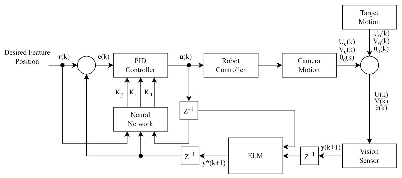
In the ELM–PID scheme, the ELM network is used to predict the system output value, which is the image Jacobian information. The structure of the ELM network is defined as six input nodes, eighteen hidden nodes and three output nodes. The input vector is $[\mathbf{u}\left(k\right),\mathbf{y}\left(k\right)]\in {\mathbf{R}}^6$, and the output vector is ${\mathbf{y}}^{*}\left(k\right)={[x\left(k\right),y\left(k\right),\omega \left(k\right)]}^T\in {\mathbf{R}}^3$. The block diagram of the ELM–PID controller is shown in Figure 2. In this scheme, $r\left(k\right)$ and $e\left(k\right)$ are the desired feature position and system error signal, respectively; $\mathbf{u}\left(k\right)$ is the PID output signal; and $\mathbf{y}\left(k\right)$ and ${\mathbf{y}}^{*}\left(k\right)$ are the output of the current and predicted feature position respectively. The tracking process of the visual servo includes the training and self-adjusting phases.

In the training phase the initial parameters of $K_P$, $K_I$ and $K_D$ are set at 10, 1 and 0.01, respectively. The robot controller is essentially an image Jacobi matrix, which describes the mapping relationship between the motion velocity of the features in image space and the robot joint angle. It guides the manipulator movement according to the input signal $\mathbf{u}$ and outputs the corresponding feature position. The sampling frequency is set to 50 ms. The collected input value $\mathbf{u}$ and output value $\mathbf{y}$ are used as the ELM’s training set. which will be normalized for the training.

In the self-adjusting phase the incremental PID algorithm is employed, and the digital PID controller can be expressed in discrete time as

$$\Delta u\left(k\right)=K_p(k-1)x_1\left(k\right)+K_i(k-1)x_2\left(k\right)+K_d(k-1)x_3\left(k\right)$$

(57)

The control law is given as

$$u\left(k\right)=u(k-1)+\Delta u\left(k\right)$$

(58)

where $\mathbf{u}$ is output of the PID controller; k is the iteration step, and

$$\left\{\begin{array}{c}e\left(k\right)=\mathbf{r}\left(k\right)-{\mathbf{y}}^{*}\left(k\right)\\ x_1=e\left(k\right)-e(k-1)\\ x_2=e\left(k\right)\\ x_3=e\left(k\right)-2e(k-1)+e(k-2)\end{array}\right.$$

(59)

The cost function of the controller is defined as

$$E\left(k\right)=\frac{1}{2}{e}^2\left(k\right)$$

(60)

During the operation, back-propagation was used to adjust the weights of the network and minimize the cost function E. The self-tuning steps are given as

$$\left\{\begin{array}{ll}\hfill \Delta K_p=-\eta & \frac{\partial E\left(k\right)}{\partial y\left(k\right)}\frac{\partial y\left(k\right)}{\partial u\left(k\right)}\frac{\partial u}{\partial K_p(k-1)}\hfill \\ \hfill & =\eta e\left(k\right)\frac{\partial y\left(k\right)}{\partial u\left(k\right)}{x}_1\left(k\right)\hfill \\ \hfill \Delta K_i=-& \eta \frac{\partial E\left(k\right)}{\partial y\left(k\right)}\frac{\partial y\left(k\right)}{\partial u\left(k\right)}\frac{\partial u}{\partial K_i(k-1)}\hfill \\ \hfill & =\eta e\left(k\right)\frac{\partial y\left(k\right)}{\partial u\left(k\right)}{x}_2\left(k\right)\hfill \\ \hfill \Delta K_d=-\eta & \frac{\partial E\left(k\right)}{\partial y\left(k\right)}\frac{\partial y\left(k\right)}{\partial u\left(k\right)}\frac{\partial u}{\partial K_d(k-1)}\hfill \\ \hfill & =\eta e\left(k\right)\frac{\partial y\left(k\right)}{\partial u\left(k\right)}{x}_3\left(k\right)\hfill \end{array}\right.$$

(61)

where $\eta$ is the learning rate, and $\frac{\partial y}{\partial u}$ is the Jacobian parameter of the visual servoing system.

Assuming that the sampling period were small enough, the two adjacent sampling points could be considered as linearly varying. Thus, we can obtain an approximation of the inverse Jacobi matrix such that

$$\frac{\partial y}{\partial u}\approx \frac{\partial y^{*}}{\partial u}=\sum _{i=1}^l{\omega }_{im}{\beta }_i{g}^{\prime }\left({\omega }_{i}u+b\right)$$

(62)

where l is the number of nodes in the hidden layer; $\beta$ is the output weight; b is the bias of the hidden layer; and ${\omega }_{im}$ is the corresponding weight in vector ${\omega }_i$ with input $\mathbf{u}$. The calculation $K_P$, $K_I$ and $K_D$ for incremental PID is given as

$$\left\{\begin{array}{l}{K}_p\left(k\right)=K_p(k-1)+\Delta K_p\left(k\right)+{\alpha }_1\left(K_p(k-1)-K_p(k-2)\right)\\ K_i\left(k\right)=K_i(k-1)+\Delta K_i\left(k\right)+{\alpha }_2\left(K_i(k-1)-K_i(k-2)\right)\\ K_d\left(k\right)=K_d(k-1)+\Delta K_d\left(k\right)+{\alpha }_3\left(K_d(k-1)-K_d(k-2)\right)\end{array}\right.$$

(63)

where $\alpha \in (0,1)$ is the momentum coefficient.

5. Experiments

As previously mentioned, this research pursued the accurate and rapid localization, and anti-disturbance capability of a line feature visual servoing. In this section, we focus on the experimental validation of the control scheme of the line feature visual servo, especially in its behavior of positioning accuracy and dynamic performance. The proposed method was validated and evaluated by testing on a six-degree-of-freedom manipulator arm. The controller code was implemented in a Robot Operating System (ROS) and the connection between the ROS and the robot was based on TCP/IP. During the tests, the tracking accuracy, the convergence speed of the feature error, the velocity component and the trajectory of the end-effector among the comparative methods will be verified.

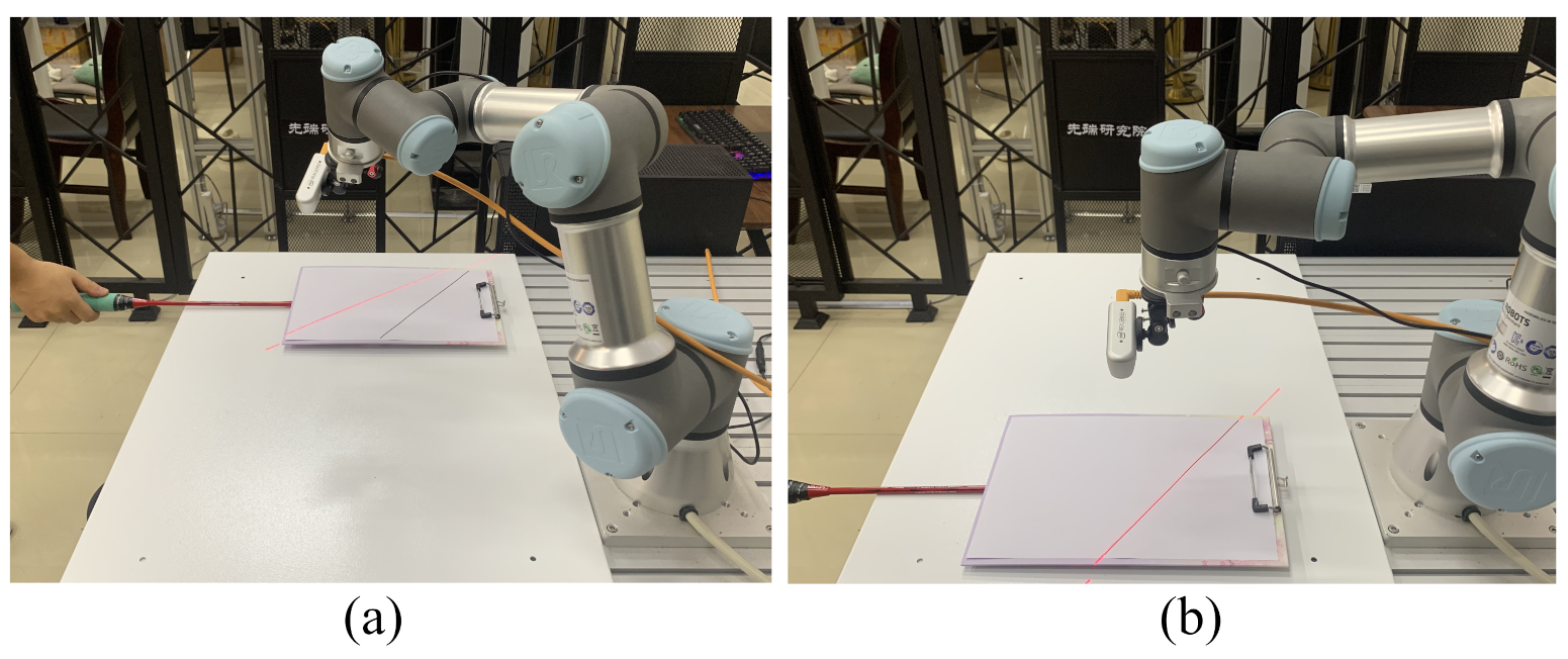
In the experiment, a black line 230 mm long and 1 mm wide was printed on paper to simulate the line features of the target. The goal of visual tracking is to control the movement of the robotic arm so that the visible red line emitted by the thlaser generator on the robot arm is aligned with the black line on the working plane. Figure 3 shows the Universal Robots UR3 robot used in this experiment. An Intel RealSense D415 RGB-D camera was used to provide RGB and depth information about the scene. Both sensors were mounted on the end-effector of the UR3 robot.

Due to the simplified representation of the target, the image lines can be identified in a straightforward way by applying the Hough transform. The block diagram of the control loop of the system is shown in Figure 2. During aligning, the target and end-effector planes are kept parallel at a distance of $Z_o$ = 680 mm. The z-axis of the camera coordinate system was perpendicular to the above two planes. The control system input was the desired position, which was the translation of the x-axis and y-axis of the camera coordinate system and the rotation of the z-axis. The unknown 3D parameters $(\theta ,\rho ,{\lambda }_{\theta },{\lambda }_{\rho })$ between the camera and the object were estimated by using the adaptive optimal predictor in Equations (31)–(33). The sampling period of the experiments was set to 50 ms.

In the first experiment, The ELM–PID controller was implemented to verify the positioning capability of the static target. Line segments printed on paper represented the line features of the target, and the projection of the laser beam on a plane was used as the current line feature, as shown in Figure 4. The robot was initialized with a specific pose, and its end-effector was 40 cm above the table. The target was placed in a random pose but always within the camera’s field of view.

In the second experiment, the performance of the ELM–PID controller in dynamic visual tracking is evaluated by using the black-lined paper to simulate the line feature of target. This piece of paper was attached to a hand grip, and random translational motions of the target were carried out by pulling the hand grip manually, as shown in Figure 5. The target was always within the camera’s field of view during the motion. The visual servoing control performance of the proposed method will be analyzed for pixel error of the image features, the convergence speed of feature error and the trajectories of motion.

6. Results

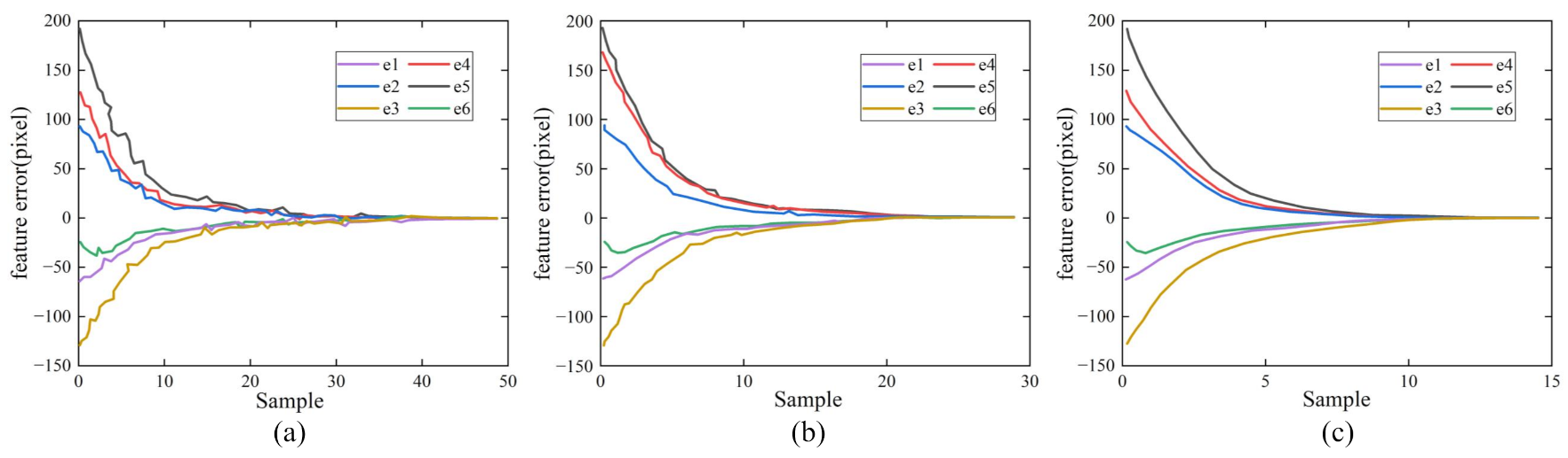
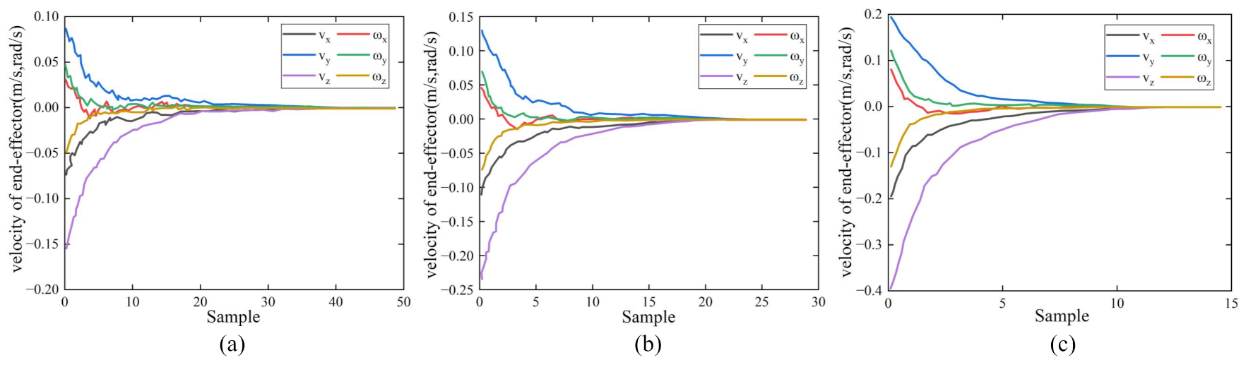
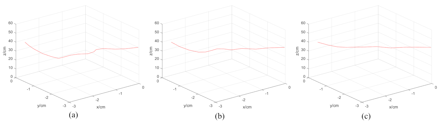
The static test of the first experiment showed that all three methods guided the robot to the target and achieve the positioning of line features. Figure 6 shows the feature error convergence curves for the current and desired features in the image plane. As shown in Figure 6a, the error convergence curve of the P controller had significant fluctuations, and convergence was completed at the 49th sample. It can be seen in Figure 6b that, the convergence curve of the PID controller was smoother than that of the P controller, which converged at the 29th sample. The ELM–PID controller had the best performance regarding the convergence curve and convergence rate, which had a smooth curve and reached the vision-servoing task at only the 14th sample. Figure 7 shows the velocity comparison of the robot’s end-effector with the three controllers. It can be seen in Figure 7a,b that, the P controller and the PID controller exhibited noticeable peaks in the motion velocity trajectory, which implied that there may be some defects in the smoothness of the robot motion. Its initial translational velocities in the x-, y- and z-axes were −0.19, 0.19, and 0.40 m/s, respectively, and the corresponding rotation velocities were 0.08, 0.12, and −0.13 rad/s, which were around 155 and 70% larger than P and PID controllers in overall initial velocity. Accordingly, we found that the motion trajectory of the robot arm showed some jitter from Figure 8a,b. In Figure 8c, it can be seen that the ELM–PID algorithm had a larger initial motion velocity, faster convergence, and smoother motion velocity profile of the end-effector. The Cartesian space motion trajectory of the ELM–PID algorithm was also much closer to a straight line, as shown in Figure 8c.

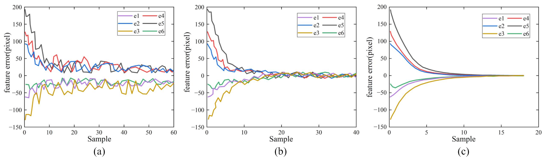
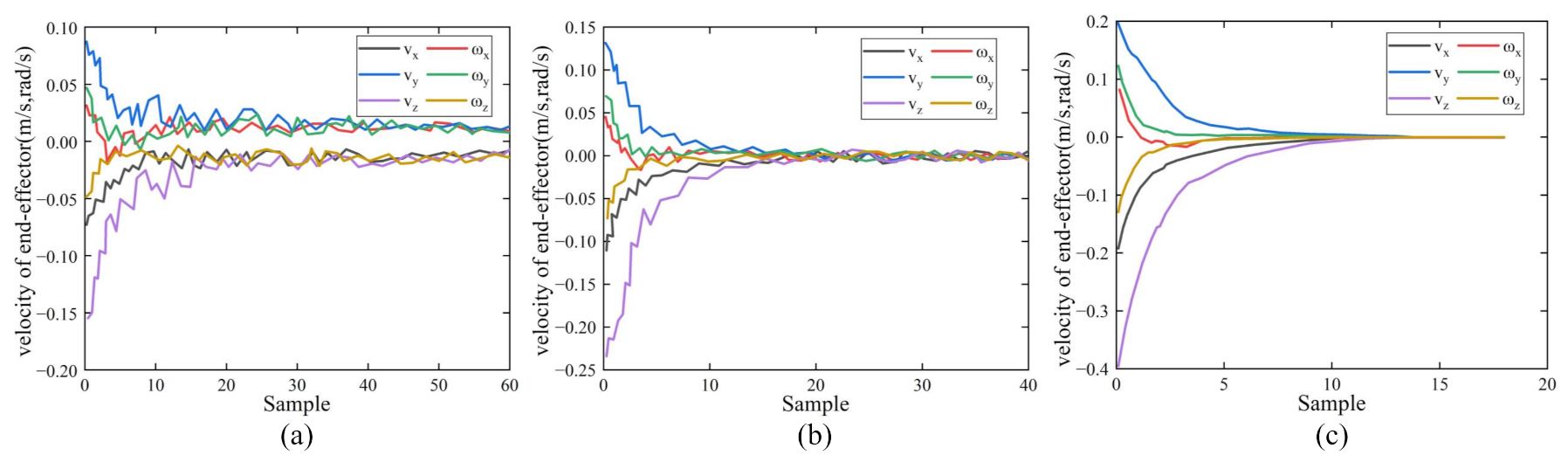
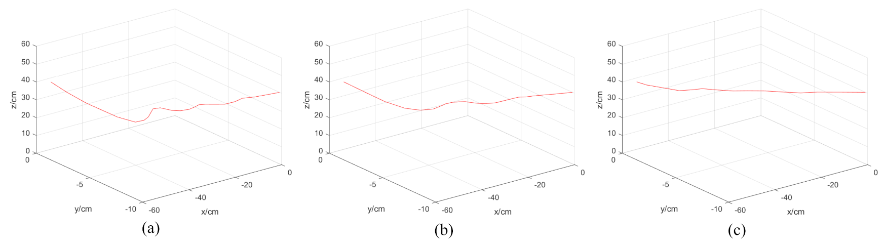
The dynamic tests of the second experiment showed that the ELM–PID controller had superior visual tracking performance for moving objects. Figure 9 illustrates the convergence curves of the feature error in the image plane between the current and reference features. Since the target was in constant motion, the feature error convergence curve was degraded compared to the first experiment. As shown in Figure 9a, the feature error curve of the P controller had noticeable jitter and failed to converge. Figure 9b shows that the convergence curve of the PID controller was more stable than that of the P controller, but the convergence took longer to complete. The ELM–PID controller had an ideal curve and converged faster, reaching the vision servo task at the 18th sample step. Figure 10 shows the velocity comparison of the end-effector corresponding to the above three vision controllers. It can be seen in Figure 10a,b that, prominent jagged peaks appeared in the motion velocity trajectories of the P and PID controller, which suggested that the robot motion process had poor smoothness. The ELM–PID algorithm improved the stability of the velocity components of the end-effector, as shown in Figure 10c. The ELM–PID still has a larger initial velocity and steeper velocity convergence curves in the dynamic test. Its initial translational velocities in the x-, y- and z-axis were −0.19, 0.19 and 0.40 m/s, respectively, and the corresponding rotational velocities were 0.08, 0.12 and −0.13 rad/s, which outperformed the P and PID controllers by around 156 and 71% in overall initial velocity. Figure 11 shows that the Cartesian space motion trajectory of the ELM–PID algorithm was closer to a straight line, and the path length was distinctly shorter than the previous two.

In essence, the P controller had substantial limitations and poor following performance in the dynamic vision tracking tasks. Although the pure PID controller accomplished dynamic vision servoing, the tracking efficiency was unsatisfactory, which may be because of the PID parameters were not in the first-rank interval. The ELM–PID exhibited the optimal error accuracy and convergence speed, steadier speed performance and faster speed convergence in both the static and dynamic vision tracking tests. The end-effector’s trajectory profile further indicated that it had fewer redundant kinematic trajectories.

7. Conclusions

This paper proposed a hybrid ELM–PID control approach for real-time robotic visual tracking of a moving target. The system consists of a visual feedback controller with self-adjusting capabilities. The image processing and camera control are performed in parallel online. The approach uses an adaptive predictor to estimate the 3D-related parameters between the camera and the object in motion. The processing of the camera image necessitates the vision sampling periods to be 50 ms and the motion of the object is assumed to be smooth. Since the dynamics of the object are unknown, the velocity and position of the object determined from the successive images are predicted using an ARMAX model. The desired trajectory points are generated online based on the relative position and velocity of the camera and the object. The online planner determines the desired trajectory points (sub-goal) one sampling period ahead. The ELM–PID controller is then constructed for visual tracking of static and moving targets. Comparing the visual servo methods based on the P and PID controller, the ELM–PID controller demonstrated the optimal visual tracking capability in both the static and dynamic tracking tests. By this method, online estimation of image Jacobi matrices was performed with an extreme learning machine, which overcame the long training time of traditional neural networks and solved the singularity of the Jacobi matrices. The gradient descent algorithm was also used to adjust the PID controller parameters adaptively, improving the controller’s dynamic performance. The principal contributions of this work are as follows:

• We developed a mathematical expression for the visual tracking of a line feature. This model was based on measurements of the vector of discrete displacements obtained by a laser-camera system;
• We presented the self-tuning control scheme of a hybrid ELM–PID. The scheme was efficient for a nonlinear system and objects in motion by composing an ELM–PID control and adaptive prediction;
• The constructed laser camera system was able to achieve low-cost, real-time vision tracking. The comprehensive experiments validated the suitability of the method for vision tracking with combined vision and control.

In future work, an attempt would be made to transplant the algorithm to industrial robots and to further tune and optimize the algorithm in industrial scenes.

References

- Castelli, F.; Michieletto, S.; Ghidoni, S.; Pagello, E. A machine learning-based visual servoing approach for fast robot control in industrial setting. Int. J. Adv. Robot. Syst. 2017, 14, 1729881417738884. [Google Scholar] [CrossRef]
- Hutchinson, S.; Hager, G.; Corke, P. Visual servoing with hand-eye manipulator-optimal control approach. IEEE Trans. Robot. Autom. 1996, 12, 651–670. [Google Scholar] [CrossRef]
- Chaumette, F.; Hutchinson, S. Visual servo control. I. Basic approaches. IEEE Robot. Autom. Mag. 2006, 13, 82–90. [Google Scholar] [CrossRef]
- Chaumette, F.; Hutchinson, S. Visual servo control. II. Advanced approaches [Tutorial]. IEEE Robot. Autom. Mag. 2007, 14, 109–118. [Google Scholar] [CrossRef]
- Wang, H.; Cheah, C.C.; Ren, W.; Xie, Y. Passive separation approach to adaptive visual tracking for robotic systems. IEEE Trans. Control Syst. Technol. 2018, 26, 2232–2241. [Google Scholar] [CrossRef]
- Liu, H.; Zhu, W.; Dong, H.; Ke, Y. Hybrid visual servoing for rivet-in-hole insertion based on super-twisting sliding mode control. Int. J. Control Autom. Syst. 2020, 18, 2145–2156. [Google Scholar] [CrossRef]
- Indrazno, S.; Laxmidhar, B.; McGinnity, T.; Sonya, C. Image-based visual servoing of a 7-DOF robot manipulator using an adaptive distributed fuzzy PD controller. IEEE Trans. Mechatron. 2014, 19, 512–523. [Google Scholar]
- Jardine, P.T.; Kogan, M.; Givigi, S.N.; Yousefi, S. Adaptive predictive control of a differential drive robot tuned with reinforcement learning. Int. J. Adapt. Control Signal Process. 2019, 33, 410–423. [Google Scholar] [CrossRef]
- Bhatti, O.S. Adaptive fuzzy-pd tracking controller for optimal visual-servoing of wheeled mobile robots. J. Control Eng. Appl. Inform. 2017, 19, 58–68. [Google Scholar]
- Yang, C.; Chen, J.; Ju, Z.; Annamalai, A.S. Visual servoing of humanoid dual-arm robot with neural learning enhanced skill transferring control. Int. J. Humanoid Robot. 2018, 15, 1750023. [Google Scholar] [CrossRef]
- Chang, T.Y.; Chang, W.C.; Cheng, M.Y.; Yang, S.S. Dynamic visual servoing with Kalman filter-based depth and velocity estimator. Int. J. Adv. Robot. Syst. 2021, 18, 17298814211016674. [Google Scholar] [CrossRef]
- Gongye, Q.; Cheng, P.; Dong, J. Image-based visual servoing with depth estimation. Trans. Inst. Meas. Control 2022, 44, 1811–1823. [Google Scholar] [CrossRef]
- Musić, J.; Bonković, M.; Cecić, M. Comparison of uncalibrated model-free visual servoing methods for small-amplitude movements: A simulation study. Int. J. Adv. Robot. Syst. 2014, 11, 108. [Google Scholar] [CrossRef]
- Durdevic, P.; Ortiz-Arroyo, D. A deep neural network sensor for visual servoing in 3d spaces. Sensors 2020, 20, 1437. [Google Scholar] [CrossRef]
- Shi, H.; Wu, H.; Xu, C.; Zhu, J.; Hwang, M.; Hwang, K.S. Adaptive image-based visual servoing using reinforcement learning with fuzzy state coding. IEEE Trans. Fuzzy Syst. 2020, 28, 3244–3255. [Google Scholar] [CrossRef]
- Qu, J.; Zhang, F.; Fu, Y.; Li, G.; Guo, S. Adaptive neural network visual servoing of dual-arm robot for cyclic motion. Ind. Robot. Int. J. 2017, 44, 210–221. [Google Scholar] [CrossRef]
- Ak, A.; Topuz, V.; Ersan, E. Visual servoing application for inverse kinematics of robotic arm using artificial neural networks. Stud. Inform. Control 2018, 27, 183–190. [Google Scholar] [CrossRef]
- Shi, H.; Li, X.; Hwang, K.S.; Pan, W.; Xu, G. Decoupled visual servoing with fuzzy Q-Learning. IEEE Trans. Ind. Inform. 2016, 14, 241–252. [Google Scholar] [CrossRef]
- Muthusamy, R.; Ayyad, A.; Halwani, M.; Swart, D.; Gan, D.; Seneviratne, L.; Zweiri, Y. Neuromorphic eye-in-hand visual servoing. IEEE Access 2021, 9, 55853–55870. [Google Scholar] [CrossRef]
- Argus, M.; Hermann, L.; Long, J.; Brox, T. Flowcontrol: Optical flow based visual servoing. In Proceedings of the 2020 IEEE/RSJ International Conference on Intelligent Robots and Systems (IROS), Las Vegas, NV, USA, 25–29 October 2020; pp. 7534–7541. [Google Scholar]
- Shao, Q.; Hu, J.; Fang, Y.; Liu, W.; Qi, J.; Zhu, G.N. Image moments based visual servoing of robot using an adaptive controller. In Proceedings of the 2016 Asia-Pacific Conference on Intelligent Robot Systems (ACIRS), Tokyo, Japan, 20–22 July 2016; pp. 57–61. [Google Scholar]
- Saxena, A.; Pandya, H.; Kumar, G.; Gaud, A.; Krishna, K.M. Exploring convolutional networks for end-to-end visual servoing. In Proceedings of the 2017 IEEE International Conference on Robotics and Automation (ICRA), Singapore, 29 May–3 June 2017; pp. 3817–3823. [Google Scholar]
- Bateux, Q.; Marchand, E.; Leitner, J.; Chaumette, F.; Corke, P. Training deep neural networks for visual servoing. In Proceedings of the 2018 IEEE International Conference on Robotics and Automation (ICRA), Brisbane, Australia, 21–25 May 2018; pp. 3307–3314. [Google Scholar]
- Sadeghi, F.; Toshev, A.; Jang, E.; Levine, S. Sim2real viewpoint invariant visual servoing by recurrent control. In Proceedings of the IEEE Conference on Computer Vision and Pattern Recognition, Salt Lake City, UT, USA, 18–22 June 2018; pp. 4691–4699. [Google Scholar]
- Wu, J.; Jin, Z.; Liu, A.; Yu, L.; Yang, F. A survey Of learning-Based control of robotic visual servoing systems. J. Frankl. Inst. 2022, 359, 556–577. [Google Scholar] [CrossRef]
- Andreff, N.; Espiau, B.; Horaud, R. Visual servoing from lines. Int. J. Robot. Res. 2002, 21, 679–699. [Google Scholar] [CrossRef]
- Wang, H.; Liu, Y.H.; Zhou, D. Adaptive visual servoing using point and line features with an uncalibrated eye-in-hand camera. IEEE Trans. Robot. 2008, 24, 843–857. [Google Scholar] [CrossRef]
- Huang, G.B.; Zhu, Q.Y.; Siew, C.K. Extreme learning machine: Theory and applications. Neurocomputing 2006, 70, 489–501. [Google Scholar] [CrossRef]
- Liao, S.; Feng, C. Meta-ELM: ELM with ELM hidden nodes. Neurocomputing 2014, 128, 81–87. [Google Scholar] [CrossRef]
- Zou, W.; Yao, F.; Zhang, B.; Guan, Z. Improved Meta-ELM with error feedback incremental ELM as hidden nodes. Neural Comput. Appl. 2018, 30, 3363–3370. [Google Scholar] [CrossRef]
Figure 1.
Configuration of the laser-camera system with a camera and a laser stripe generator.
Figure 2.
Block diagram of adaptive visual tracking system with ELM–PID controller.
Figure 3.
The experimental platform of visual servoing tracking.
Figure 4.
Experiment 1: Static positioning with line features. (a) The robot’s pose before attempting to reach the goal. (b) The robot in the goal state.
Figure 5.
Experiment 2: dynamic target tracking trials. (a) The laser line and the black line are not yet aligned, and the robot is tracking. (b) The laser line and the black line are aligned, and the robot is in the goal state.
Figure 6.
Comparison of image feature errors of the three controllers on the static positioning test. (a) P controller. (b) PID controller. (c) ELM–PID controller.
Figure 7.
Comparison of robot’s end-effector velocities of the three controllers on the static positioning test. (a) P controller. (b) PID controller. (c) ELM–PID controller.
Figure 8.
Comparison of the robot’s end-effector trajectory of the three controllers on the static positioning test. (a) P controller. (b) PID controller. (c) ELM–PID controller.
Figure 9.
Comparison of image feature errors of the three controllers on the dynamic visual tracking test. (a) P controller. (b) PID controller. (c) ELM–PID controller.
Figure 10.
Comparison of robot’s end-effector velocities of the three controllers on the dynamic visual tracking test. (a) P controller. (b) PID controller. (c) ELM–PID controller.
Figure 11.
Comparison of robot’s end-effector trajectory of the three controllers on the dynamic visual tracking test. (a) P controller. (b) PID controller. (c) ELM–PID controller.
Publisher’s Note: MDPI stays neutral with regard to jurisdictional claims in published maps and institutional affiliations. |
© 2022 by the authors. Licensee MDPI, Basel, Switzerland. This article is an open access article distributed under the terms and conditions of the Creative Commons Attribution (CC BY) license (https://creativecommons.org/licenses/by/4.0/).
Share and Cite
MDPI and ACS Style
Luo, J.; Zhu, L.; Wu, N.; Chen, M.; Liu, D.; Zhang, Z.; Liu, J. Adaptive Neural-PID Visual Servoing Tracking Control via Extreme Learning Machine. Machines 2022, 10, 782. https://doi.org/10.3390/machines10090782
AMA Style
Luo J, Zhu L, Wu N, Chen M, Liu D, Zhang Z, Liu J. Adaptive Neural-PID Visual Servoing Tracking Control via Extreme Learning Machine. Machines. 2022; 10(9):782. https://doi.org/10.3390/machines10090782
Chicago/Turabian StyleLuo, Junqi, Liucun Zhu, Ning Wu, Mingyou Chen, Daopeng Liu, Zhenyu Zhang, and Jiyuan Liu. 2022. "Adaptive Neural-PID Visual Servoing Tracking Control via Extreme Learning Machine" Machines 10, no. 9: 782. https://doi.org/10.3390/machines10090782
Note that from the first issue of 2016, this journal uses article numbers instead of page numbers. See further details here.