

Fourier-Based Adaptive Signal Decomposition Method Applied to Fault Detection in Induction Motors
 , ,
, ,  ,
, 
Abstract
:1. Introduction
2. Materials and Methods
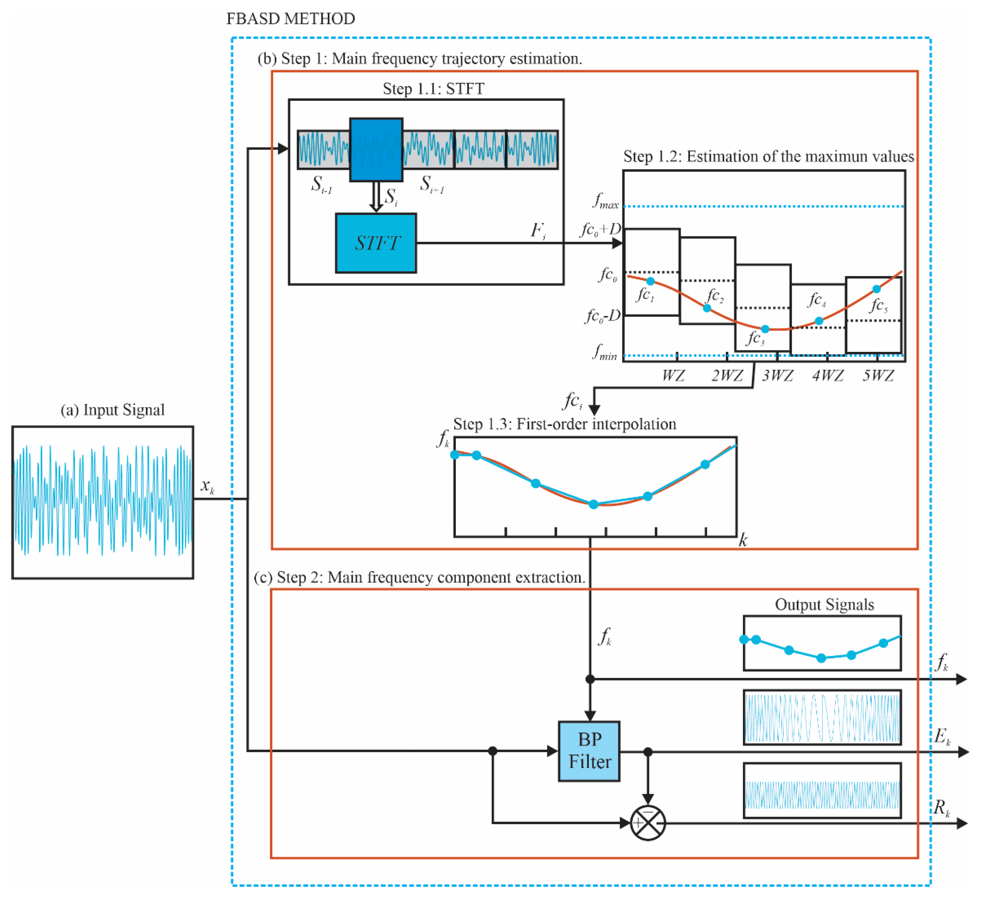
2.1. Fourier-Based Adaptive Signal Decomposition (FBASD)
2.1.1. Step 1. Main Frequency Trajectory Estimation
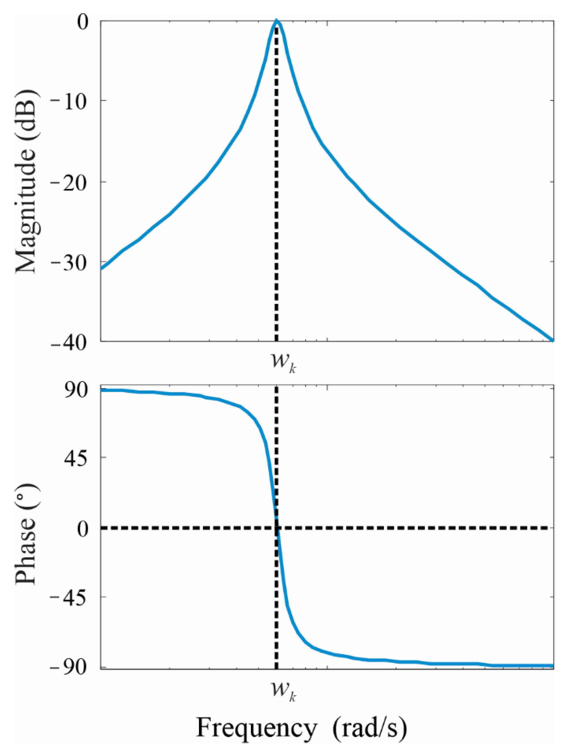
2.1.2. Step 2. Main Frequency Component Extraction
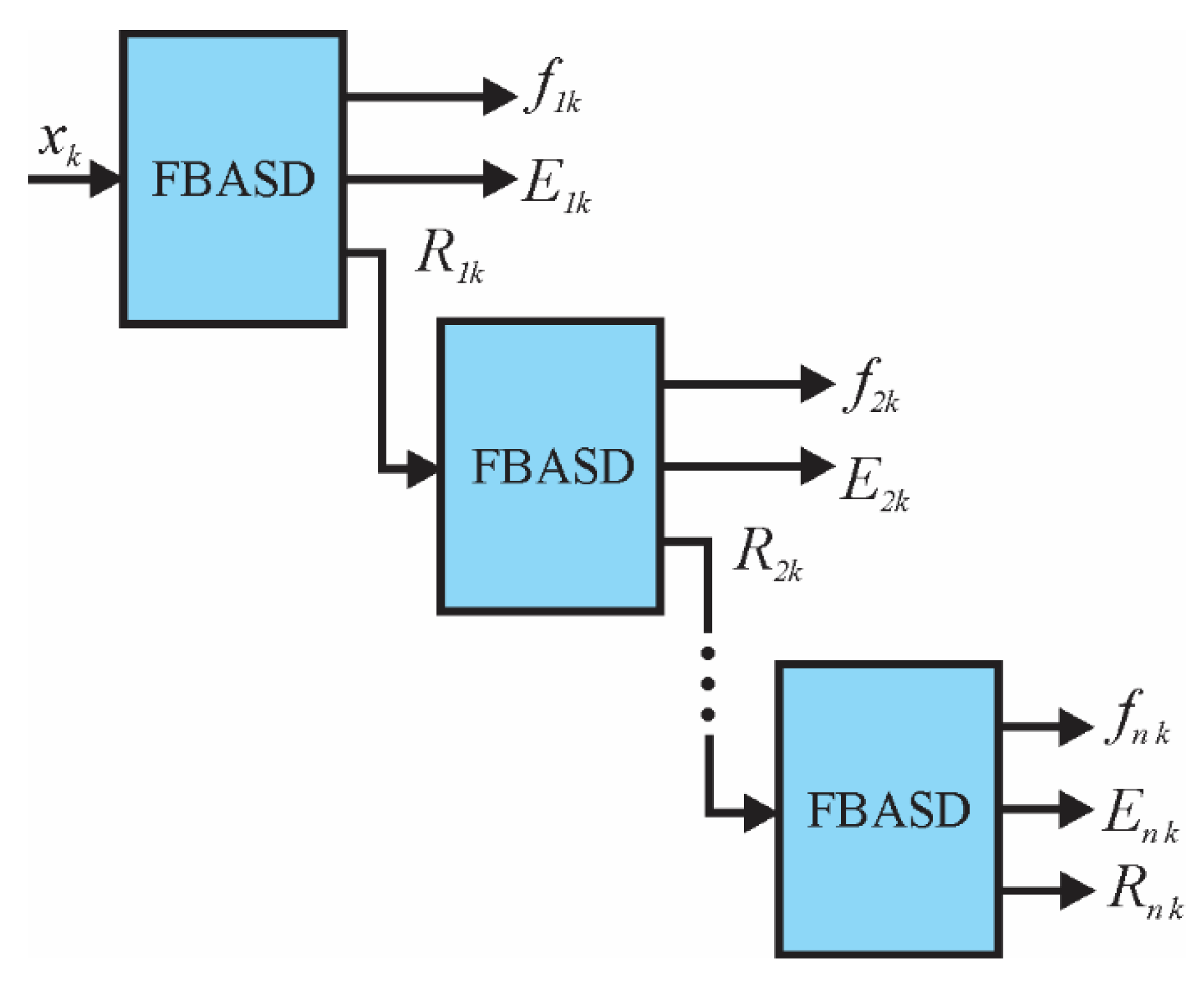
2.2. Extraction of N Time-Frequency Components
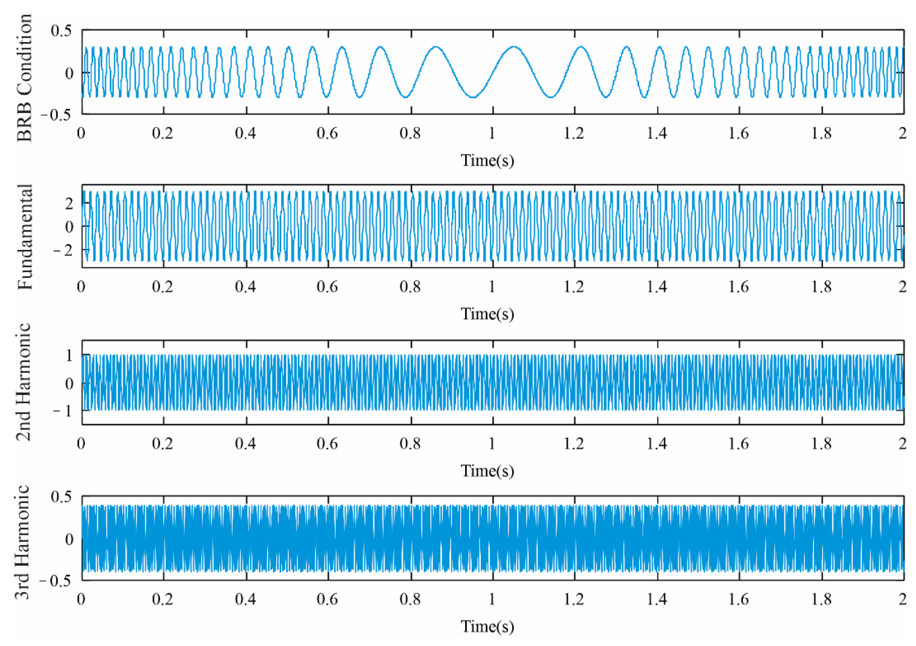
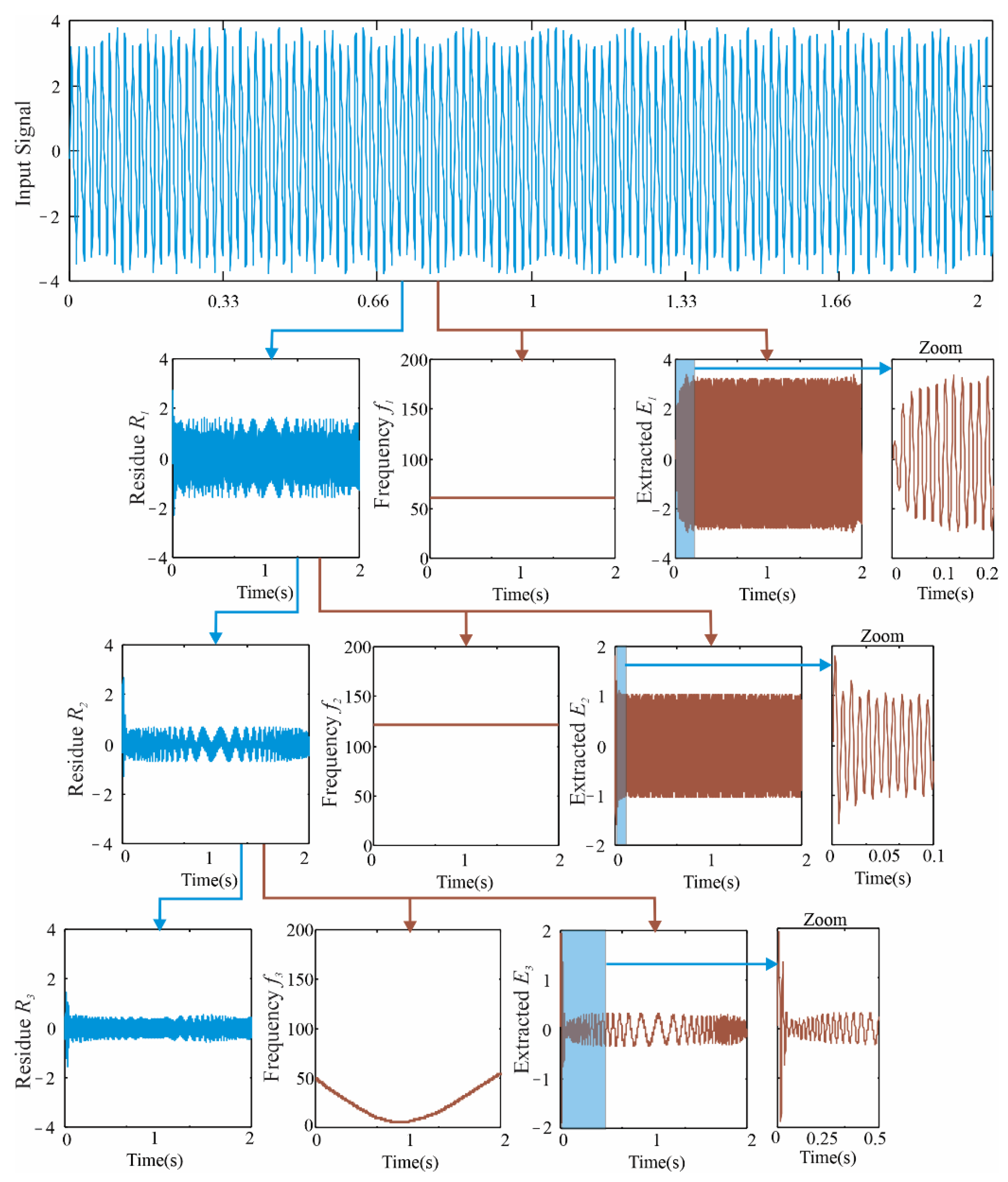
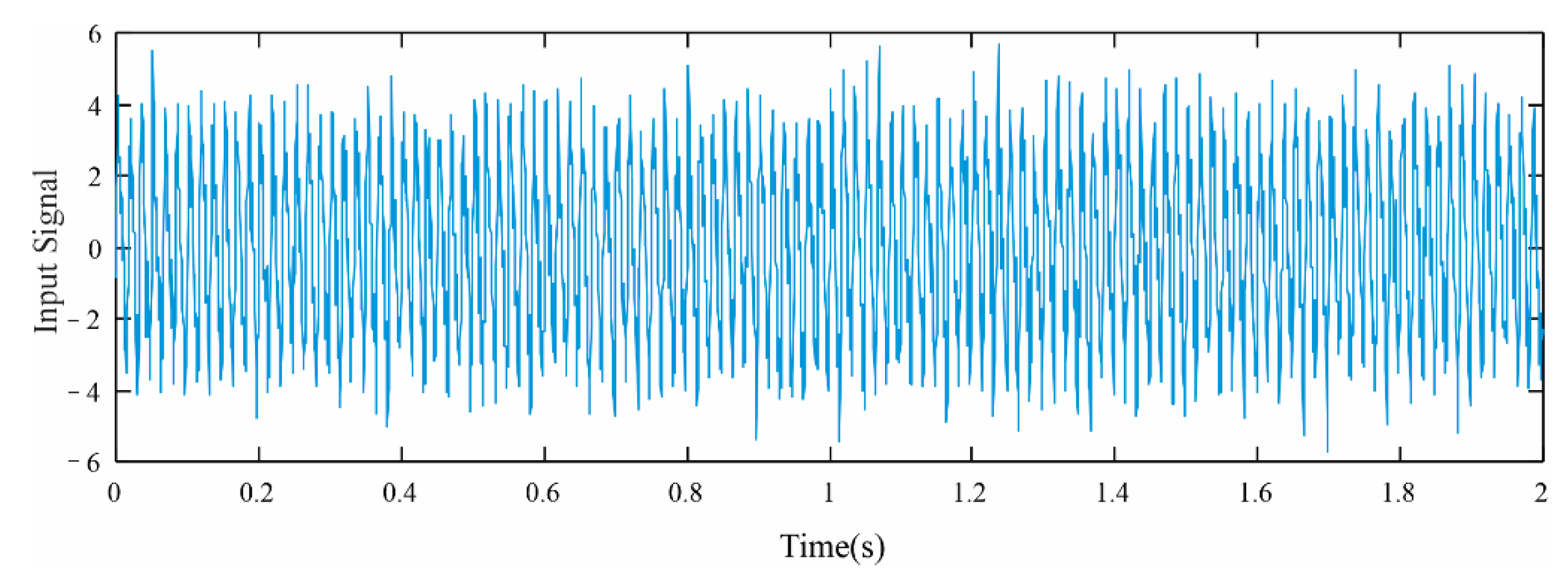
2.3. Simulation
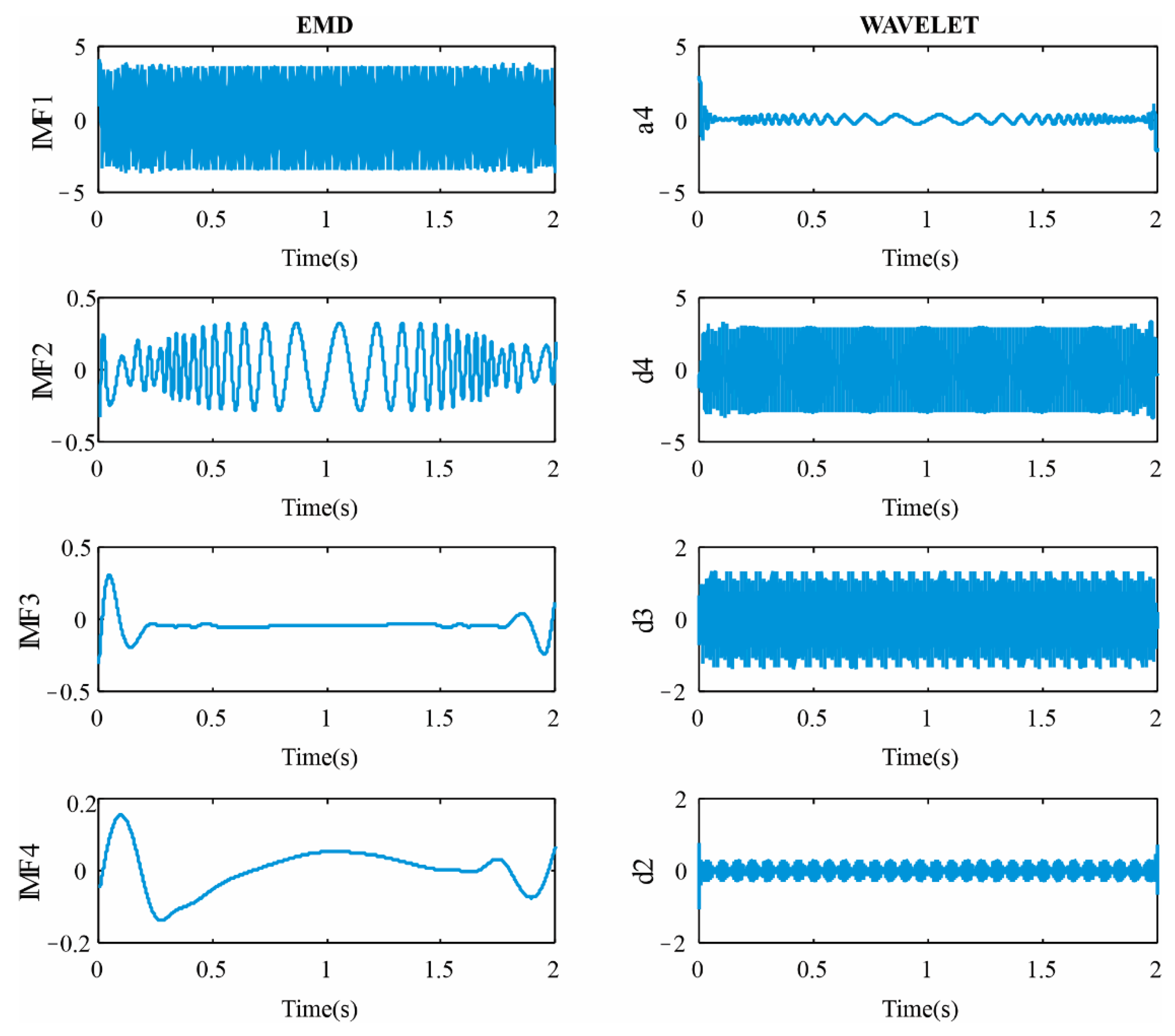
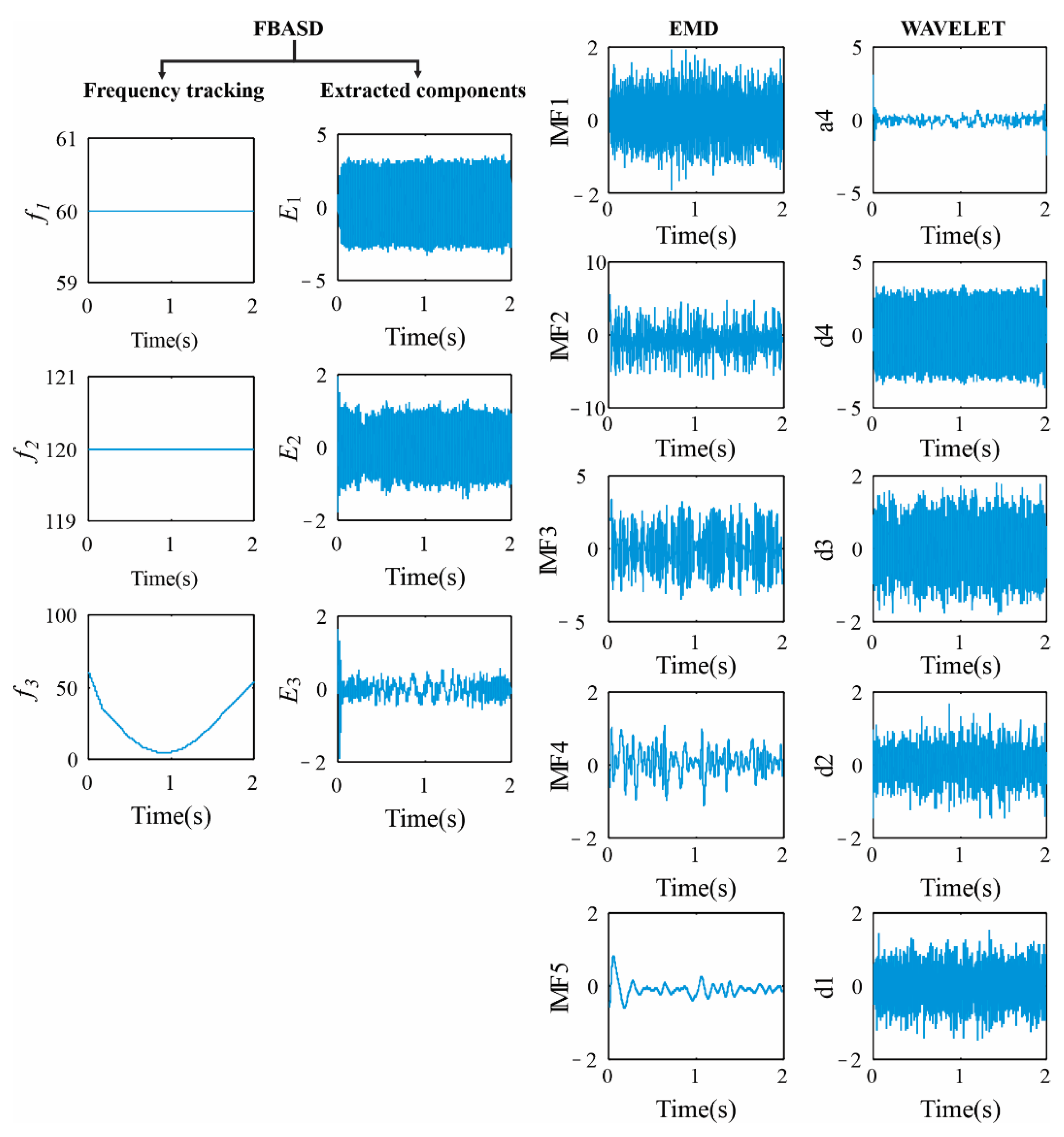
2.4. Comparison
3. Results
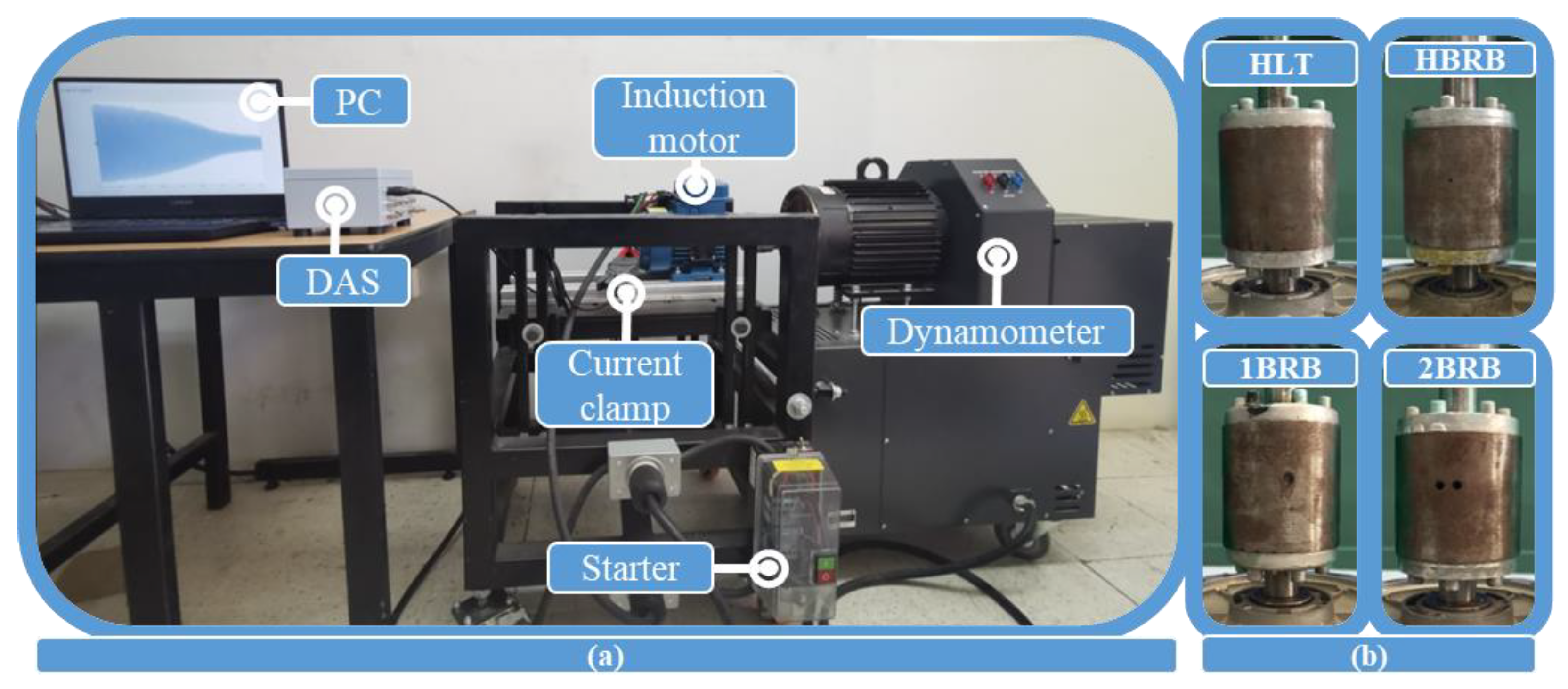
3.1. Experimental Setup
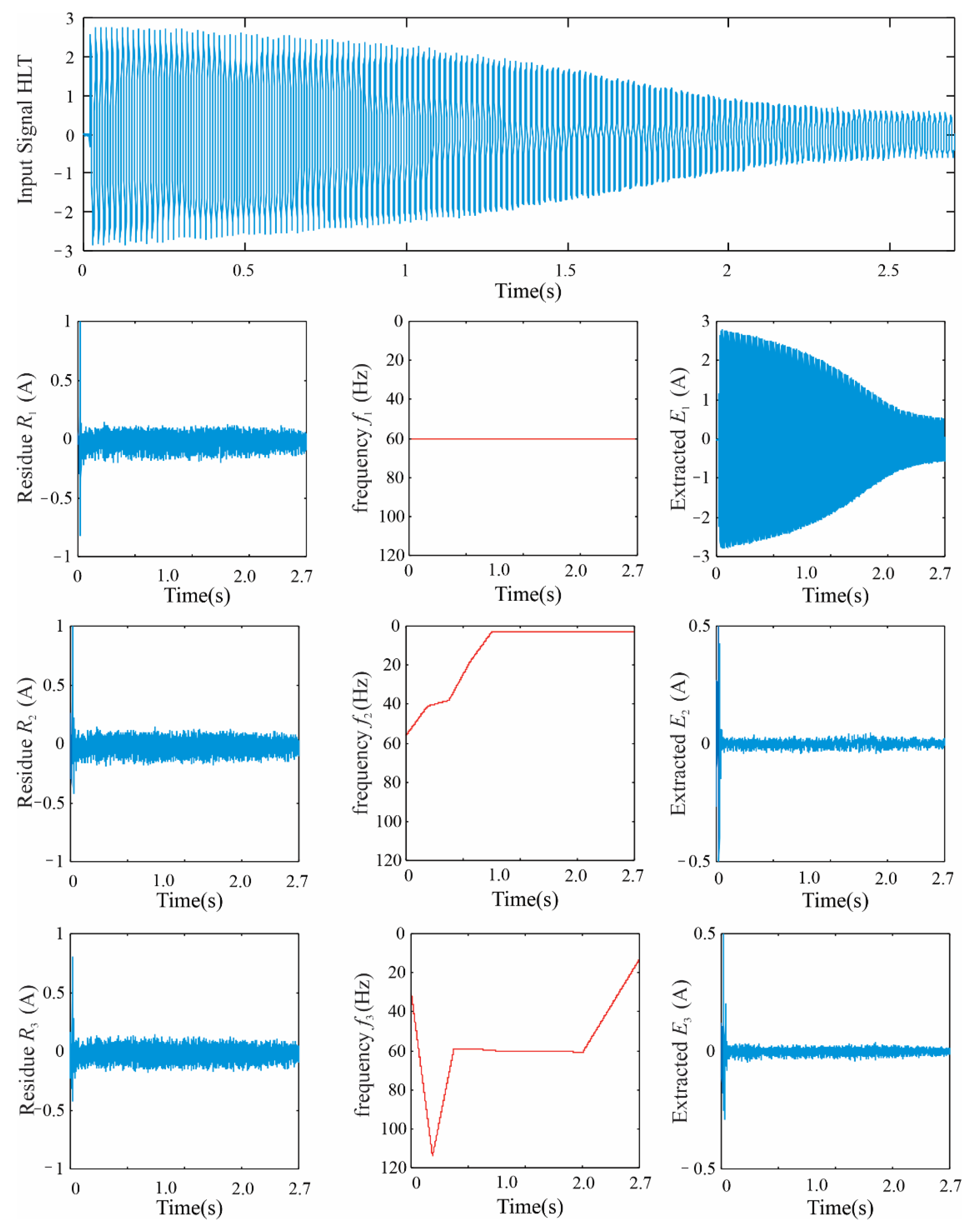
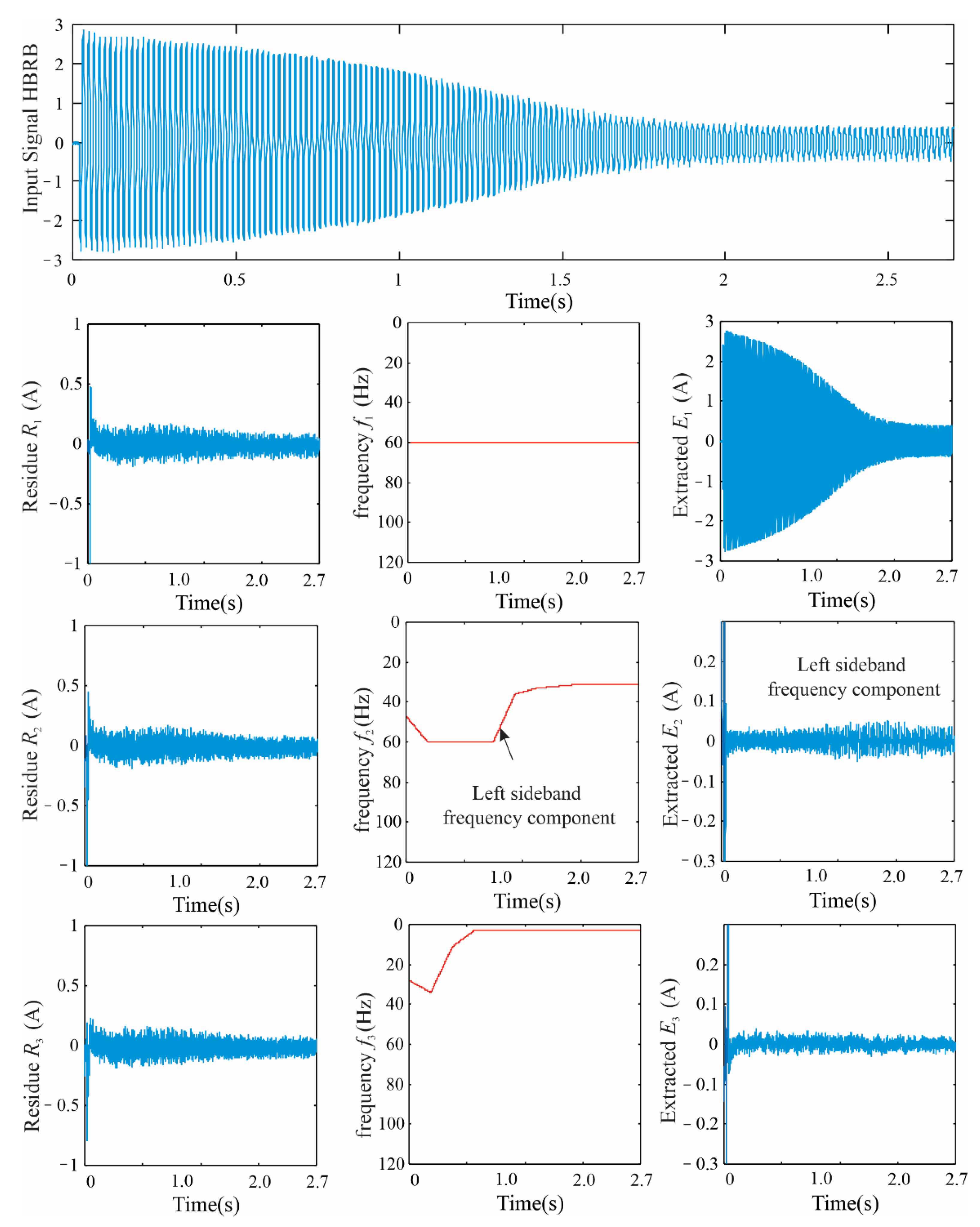
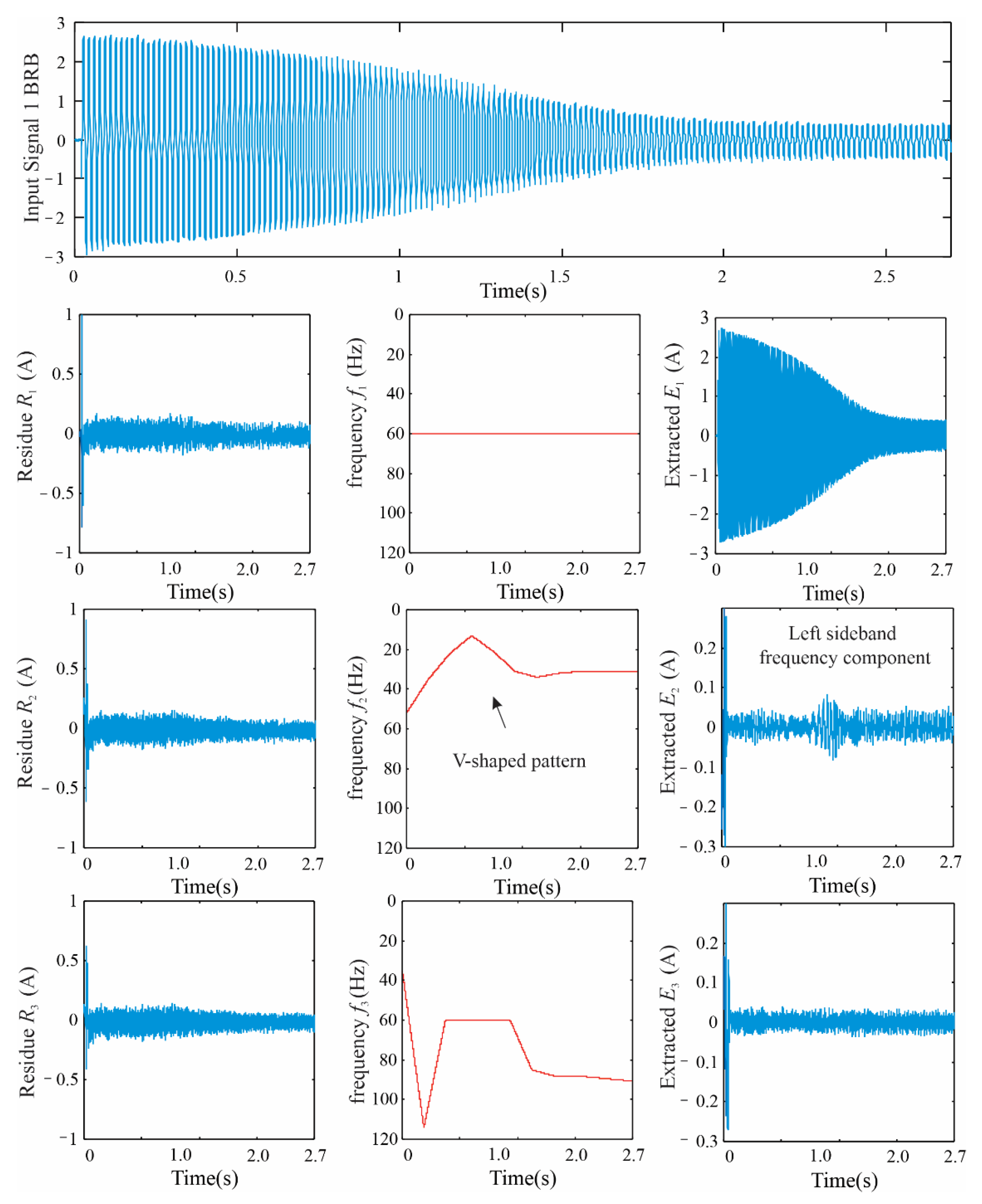
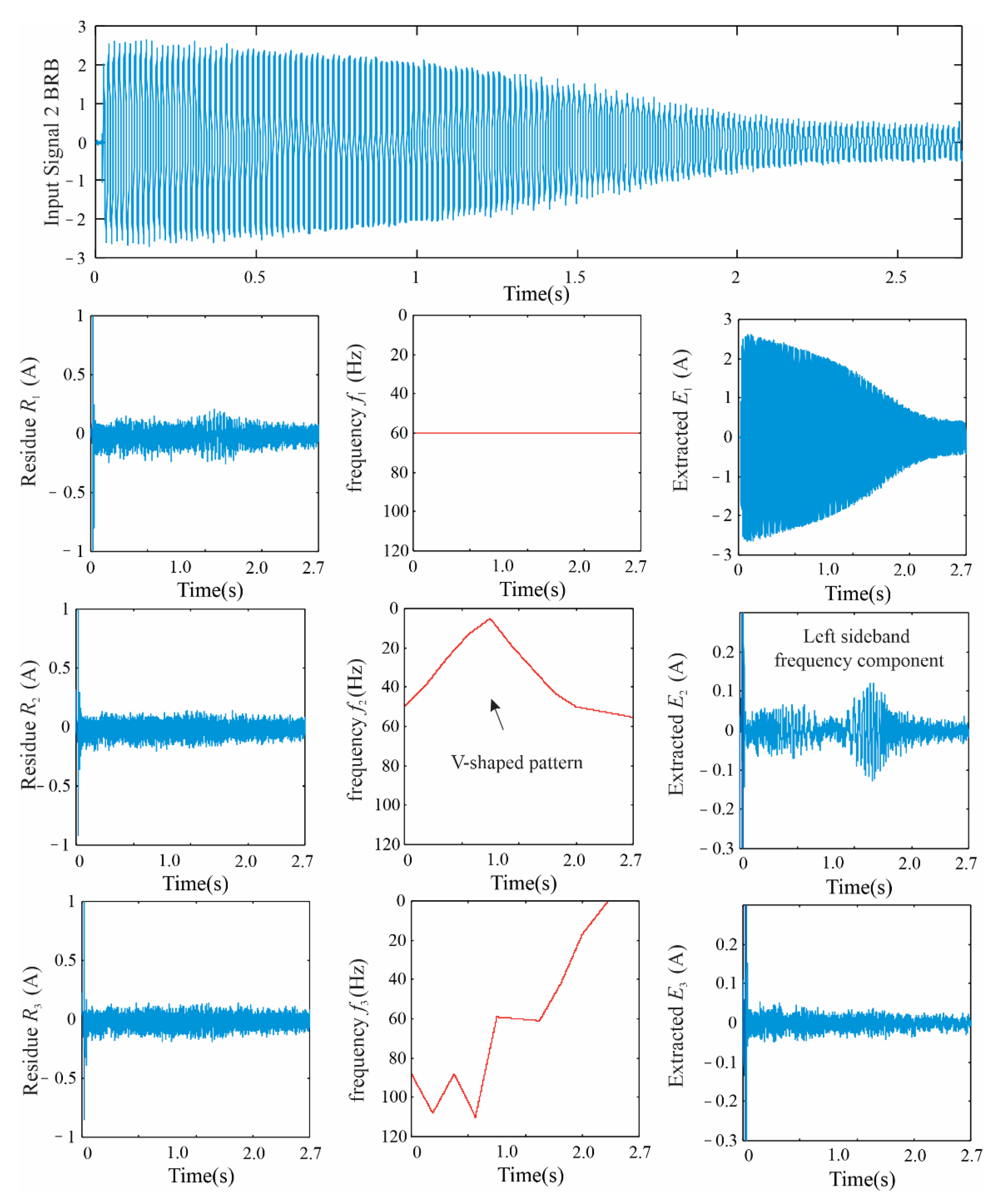
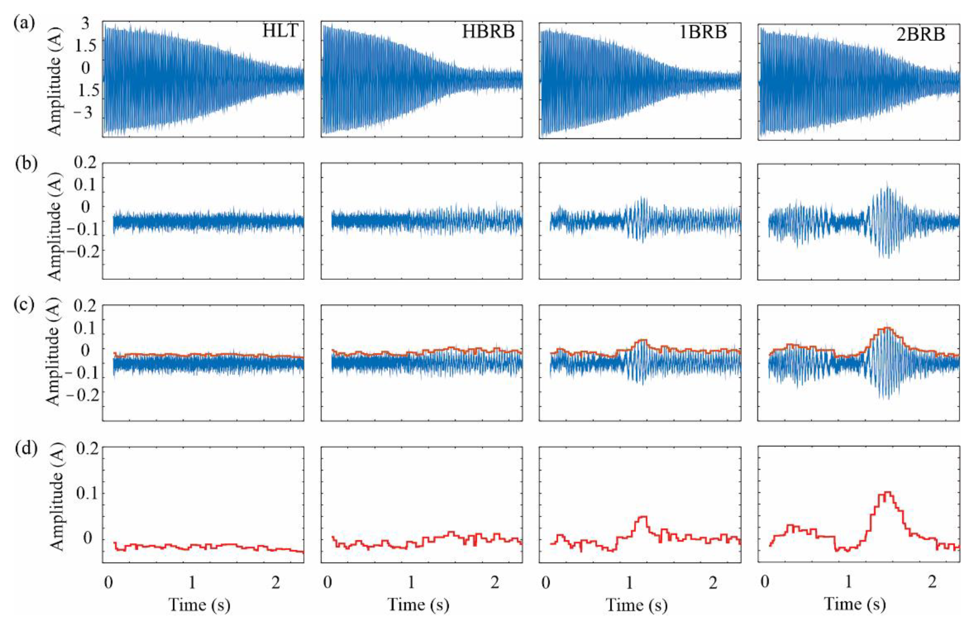
3.2. FBASD Results
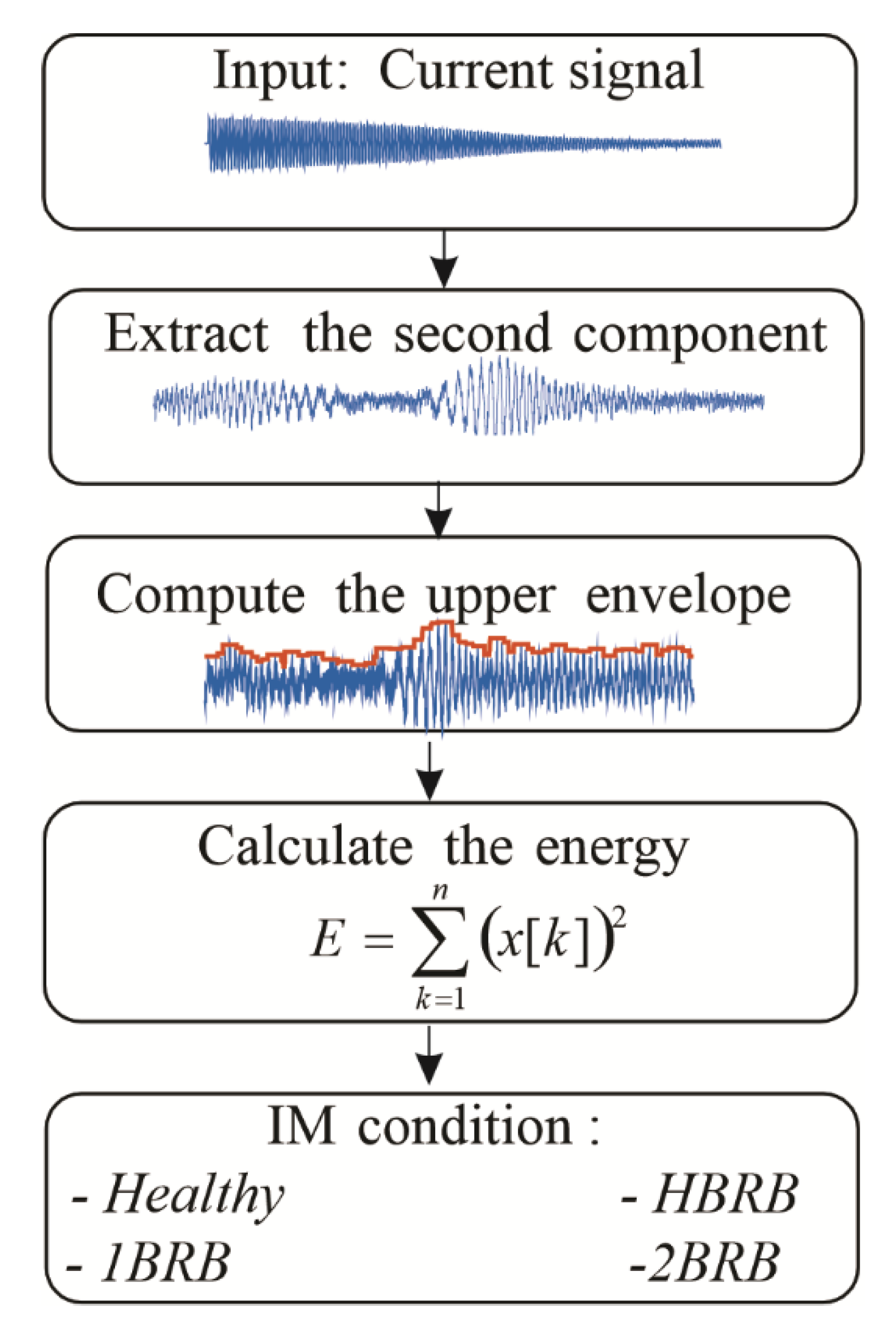
3.3. Classification Algorithm
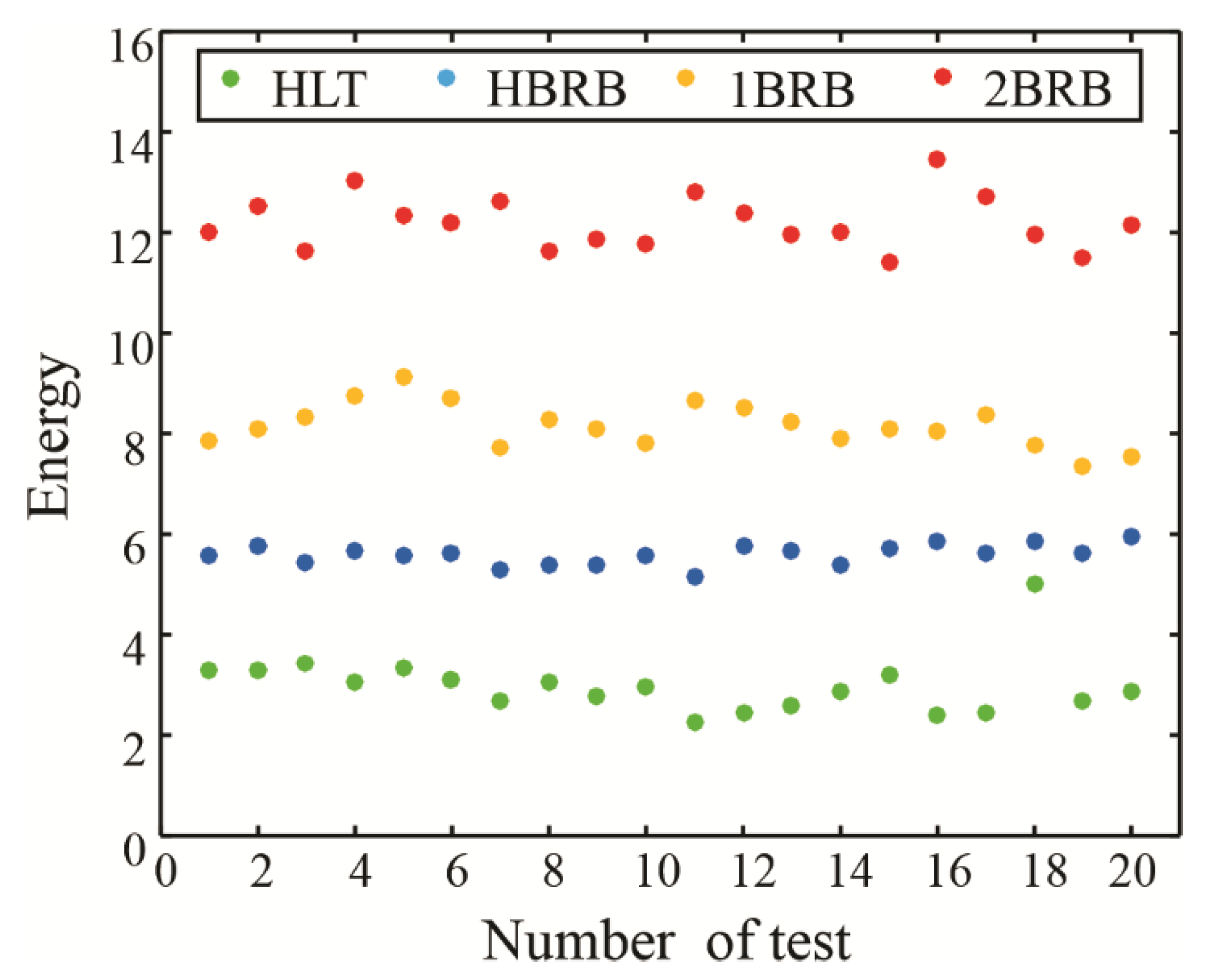
3.4. Classification Results
4. Discussion
5. Conclusions
Author Contributions
Funding
Institutional Review Board Statement
Informed Consent Statement
Data Availability Statement
Conflicts of Interest
References
- Bilal, A.; Toomas, V.; Anton, R.; Ants, K.; Anouar, B. A survey of broken rotor bar fault diagnostic methods of induction motor. Electr. Cont. Comm. Eng. 2018, 14, 117–124. [Google Scholar]
- Huang, L.; Hu, N.; Yang, Y.; Chen, L.; Wen, J.; Shen, G. Study on Electromagnetic-Dynamic Coupled Modeling Method-Detection by Stator Current of the Induction Motors with Bearing Faults. Machines 2022, 10, 682. [Google Scholar] [CrossRef]
- Chen, P.; Xie, Y.; Li, D. Thermal Field and Stress Analysis of Induction Motor with Stator Inter-Turn Fault. Machines 2022, 10, 504. [Google Scholar] [CrossRef]
- Gonzalez-Cordoba, J.L.; Granados-Lieberman, D.; Osornio-Rios, R.A.; Romero-Troncoso, R.J.; de Santiago-Perez, J.J.; Valtierra-Rodriguez, M. Methodology for overheating identification on induction motors under voltage unbalance conditions in industrial processes. J. Sci. Ind. Res. 2016, 75, 100–107. [Google Scholar]
- Lamim-Filho, P.C.M.; Baccarini, L.M.R.; Batista, F.B.; Alves, D.A. Broken rotor bar detection using empirical demodulation and wavelet transform: Suitable for industrial application. Electr. Eng. 2018, 100, 2253–2260. [Google Scholar] [CrossRef]
- Miljković, D. Brief review of motor current signature analysis. HDKBR INFO Mag. 2015, 5, 14–26. [Google Scholar]
- Rivera-Guillen, J.R.; de Santiago-Perez, J.J.; Amezquita-Sanchez, J.P.; Valtierra-Rodriguez, M.; Romero-Troncoso, R.J. Enhanced FFT-based method for incipient broken rotor bar detection in induction motors during the startup transient. Measurement 2018, 124, 277–285. [Google Scholar] [CrossRef]
- Shi, P.; Chen, Z.; Vagapov, Y.; Zouaoui, Z. A new diagnosis of broken rotor bar fault extent in three phase squirrel cage induction motor. Mech. Syst. Signal Proc. 2014, 42, 388–403. [Google Scholar] [CrossRef]
- Ojaghi, M.; Sabouri, M.; Faiz, J. Performance analysis of squirrel-cage induction motors under broken rotor bar and stator inter-turn fault conditions using analytical modeling. IEEE T. Magn. 2018, 54, 8203705. [Google Scholar] [CrossRef]
- Abd-el-Malek, M.; Abdelsalam, A.K.; Hassan, O.E. Induction motor broken rotor bar fault location detection through envelope analysis of start-up current using Hilbert transform. Mech. Syst. Signal Proc. 2017, 93, 332–350. [Google Scholar] [CrossRef]
- Reis, M.S.; Gins, G. Industrial process monitoring in the big data/industry 4.0 era: From detection, to diagnosis, to prognosis. Processes 2017, 5, 35. [Google Scholar] [CrossRef]
- Cusido, J.; Rosero, J.; Aldabas, E.; Ortega, J.A.; Romeral, L. New fault detection techniques for induction motors. Electr. Pow. Q. Util. Mag. 2006, 2, 39–46. [Google Scholar]
- Sharma, A.; Verma, P.; Mathew, L.; Chatterji, S. Using Motor Current Analysis for Broken Rotor Bar Fault Detection in Rotary Machines. In Proceedings of the International Conference on Communication and Electronics Systems, Coimbatore, India, 15–16 October 2018; pp. 329–334. [Google Scholar]
- Sinha, A.K.; Hati, A.S.; Benbouzid, M.; Chakrabarti, P. ANN-Based Pattern Recognition for Induction Motor Broken Rotor Bar Monitoring under Supply Frequency Regulation. Machines 2021, 9, 87. [Google Scholar] [CrossRef]
- Mazouji, R.; Khaloozadeh, H.; Arasteh, M. Fault Diagnosis of Broken Rotor Bars in Induction Motors Using Finite Element Analysis. In Proceedings of the IEEE Power Electronics, Drive Systems, and Technologies Conference, Tehran, Iran, 4–6 February 2020; pp. 1–5. [Google Scholar]
- Chen, S.; Zivanovic, R. Estimation of frequency components in stator current for the detection of broken rotor bars in induction machines. Measurement 2010, 43, 887–900. [Google Scholar] [CrossRef]
- Souza, M.V.; Lima, J.C.O.; Roque, A.M.P.; Riffel, D.B. A Novel Algorithm to Detect Broken Bars in Induction Motors. Machines 2021, 9, 250. [Google Scholar] [CrossRef]
- Singh, G.; Naikan, V.N.A. Detection of half broken rotor bar fault in VFD driven induction motor drive using motor square current MUSIC analysis. Mech. Syst. Signal Proc. 2018, 110, 333–348. [Google Scholar] [CrossRef]
- Climente-Alarcon, V.; Antonino-Daviu, J.A.; Riera-Guasp, M.; Vlcek, M. Induction motor diagnosis by advanced notch fir filters and the wigner–ville distribution. IEEE T. Ind. Electro. 2014, 61, 4217–4227. [Google Scholar] [CrossRef]
- Eren, L.; Askar, M.; Devaney, M. Motor current signature analysis via four-channel FIR filter banks. Measurement 2016, 89, 322–327. [Google Scholar] [CrossRef]
- Liu, Y.; Guo, L.; Wang, Q.; An, G.; Guo, M.; Lian, H. Application to induction motor faults diagnosis of the amplitude recovery method combined with FFT. Mech. Syst. Signal Proc. 2010, 24, 2961–2971. [Google Scholar] [CrossRef]
- Gaeid, K.S.; Ping, H.W.; Khalid, M.; Salih, A.L. Fault diagnosis of induction motor using MCSA and FFT. Electr. Electr. Eng. 2011, 1, 85–92. [Google Scholar]
- Ameid, T.; Menacer, A.; Talhaoui, H.; Harzelli, I. Rotor resistance estimation using Extended Kalman filter and spectral analysis for rotor bar fault diagnosis of sensorless vector control induction motor. Measurement 2017, 111, 243–259. [Google Scholar] [CrossRef]
- Ayhan, B.; Trussell, H.J.; Chow, M.-Y.; Song, M.-H. On the use of a lower sampling rate for broken rotor bar detection with DTFT and AR-based spectrum methods. IEEE T. Ind. Electron. 2008, 55, 1421–1434. [Google Scholar] [CrossRef]
- Pons-Llinares, J.; Antonino-Daviu, J.A.; Riera-Guasp, M.; Pineda-Sanchez, M.; Climente-Alarcon, V. Induction motor diagnosis based on a transient current analytic Wavelet transform via frequency B-splines. IEEE T. Ind. Electron. 2011, 58, 1530–1544. [Google Scholar] [CrossRef]
- Konar, P.; Chattopadhyay, P. Bearing fault detection of induction motor using wavelet and support vector machines (SVMs). Appl. Soft. Comput. 2011, 11, 4203–4211. [Google Scholar] [CrossRef]
- Saidi, L.; Ali, J.B.; Fnaiech, F. Bi-spectrum based-EMD applied to the non-stationary vibration signals for bearing faults diagnosis. ISA T. 2014, 53, 1650–1660. [Google Scholar] [CrossRef]
- Faiz, J.; Ghorbanian, V.; Ebrahimi, B.M. EMD-based analysis of industrial induction motors with broken rotor bars for identification of operating point at different supply modes. IEEE T. Ind. Inform. 2014, 10, 957–966. [Google Scholar] [CrossRef]
- Liu, D.; Xiao, Z.; Hu, X.; Zhang, C.; Malik, O.P. Feature extraction of rotor fault based on EEMD and curve code. Measurement 2019, 135, 712–724. [Google Scholar] [CrossRef]
- Zarei, J.; Poshtan, J. Bearing fault detection using wavelet packet transform of induction motor stator current. Tribol. Int. 2007, 40, 763–769. [Google Scholar] [CrossRef]
- Keskes, H.; Braham, A. Recursive undecimated Wavelet packet transform and DAG SVM for induction motor diagnosis. IEEE T. Ind. Inform. 2015, 11, 1059–1066. [Google Scholar] [CrossRef]
- Elbouchikhi, E.; Choqueuse, V.; Benbouzid, M. Induction machine bearing faults detection based on a multi-dimensional MUSIC algorithm and maximum likelihood estimation. ISA T. 2016, 63, 413–424. [Google Scholar] [CrossRef]
- Gugaliya, A.; Singh, G.; Naikan, V.N.A. Effective combination of motor fault diagnosis techniques. In Proceedings of the International Conference on Power, Instrumentation, Control and Computing, Thrissur, India, 12–20 January 2018; pp. 1–5. [Google Scholar]
- Sadeghian, A.; Ye, Z.; Wu, B. Online detection of broken rotor bars in induction motors by Wavelet packet decomposition and artificial neural networks. IEEE T. Instrum. Meas. 2009, 58, 2253–2263. [Google Scholar] [CrossRef]
- Proakis, J.G.; Manolakis, D.G. Digital Signal Processing: Principles Algorithms and Applications, 3rd ed.; Prentice-Hall International Inc.: Hoboken, NJ, USA, 1996. [Google Scholar]
- Valtierra-Rodriguez, M.; Rivera-Guillen, J.R.; Basurto-Hurtado, J.A.; de Santiago-Perez, J.J.; Granados-Lieberman, D.; Amezquita-Sanchez, J.P. Convolutional Neural Network and Motor Current Signature Analysis during the Transient State for Detection of Broken Rotor Bars in Induction Motors. Sensors 2020, 20, 3721. [Google Scholar] [CrossRef] [PubMed]
- Huang, N.E.; Shen, Z.; Long, S.R.; Wu, M.C.; Shih, H.H.; Zheng, Q.; Yen, Z.-C.; Tung, C.C.; Liu, H.H. The empirical mode decomposition and Hilbert spectrum for nonlinear and nonstationary time series analysis. Proc. R. Soc. A 1998, 545, 903–995. [Google Scholar] [CrossRef]
- Amezquita-Sanchez, J.P.; Adeli, H. Signal processing techniques for vibration-based health monitoring of smart structures. Arch. Comput. Methods Eng. 2016, 23, 1–15. [Google Scholar] [CrossRef]
- Garcia-Calva, T.A.; Morinigo-Sotelo, D.; Fernandez-Cavero, V.; Garcia-Perez, A.; Romero-Troncoso, R.D.J. Early detection of broken rotor bars in inverter-fed induction motors using speed analysis of startup transients. Energies 2021, 14, 1469. [Google Scholar] [CrossRef]
- Benbouzid, M.E.H. A review of induction motors signature analysis as a medium for faults detection. IEEE T. Ind. Electron. 2000, 47, 984–993. [Google Scholar] [CrossRef]
- Huang, S.; Tong, Y.; Zhao, W. A denoising algorithm for an electromagnetic acoustic transducer (EMAT) signal by envelope regulation. Meas. Sci. Technol. 2010, 21, 085206. [Google Scholar] [CrossRef]


| Signal | Method | NMSE Ideal | NMSE Noisy |
|---|---|---|---|
| FBASD | 0.989 | 0.980 | |
| EMD | 0.867 | 0.364 IMF2 | |
| Wavelet | 0.987 | 0.980 | |
| FBASD | 0.830 | 0.340 | |
| EMD | 0.648 | 0.207 IMF4 | |
| Wavelet | 0.900 | 0.250 | |
| FBASD | 0.950 | 0.900 | |
| EMD | N.D. * | N.D. * | |
| Wavelet | 0.880 | 0.790 |
| Feature | FBASD | EMD | Wavelet |
|---|---|---|---|
| Basis | Semi-adaptive | Adaptive | Non-adaptive |
| Configuration parameters | Frequency range, froc | Standard deviation | Wavelet Mother, decomposition level |
| Frequency information | Yes | No | No |
| Frequency range of interest | Yes | No | Partially |
| Computing time (seconds) | 0.005 | 1.83 | 0.023 |
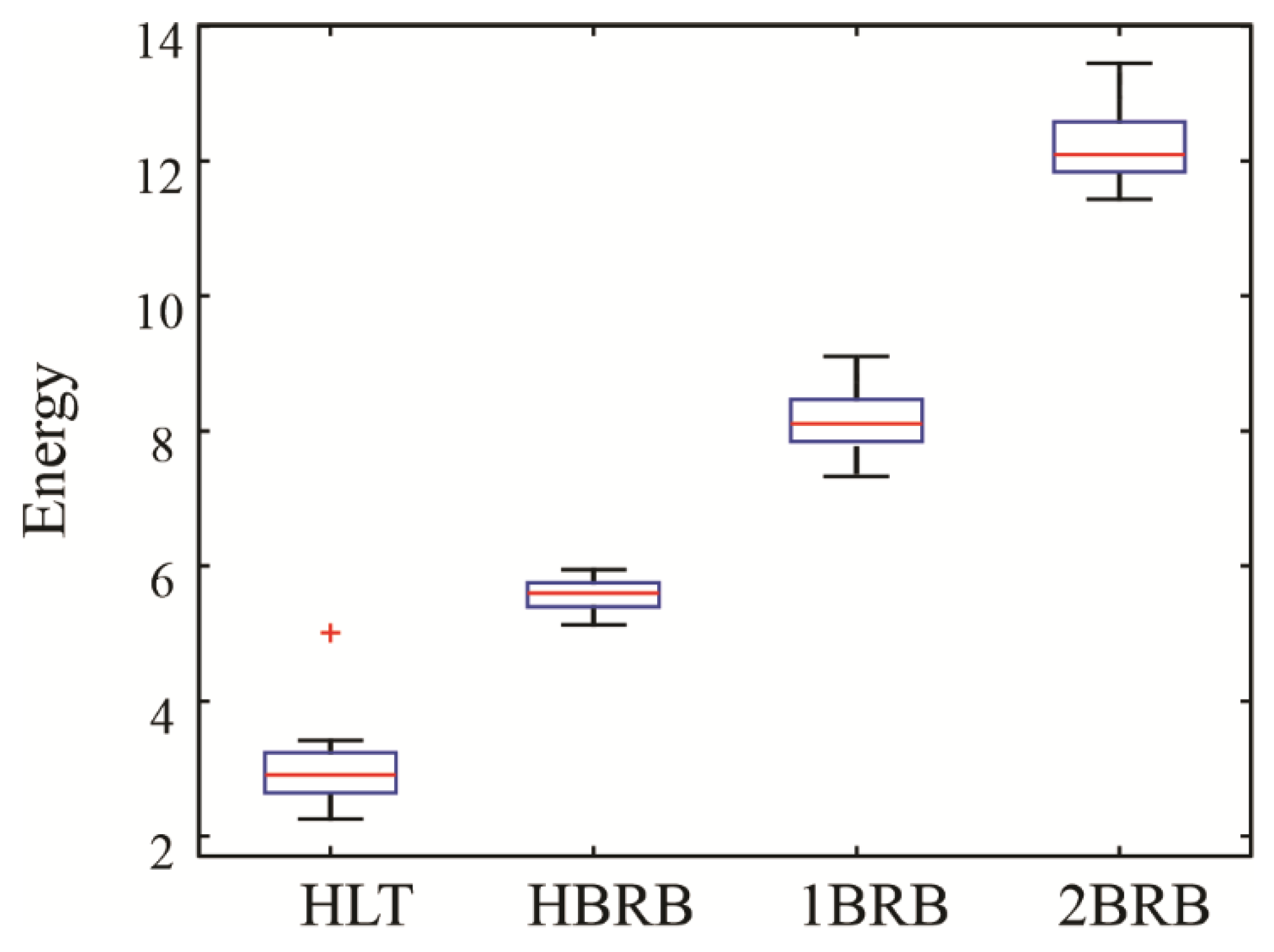
| IM Condition | Mean | Standard Deviation |
|---|---|---|
| HLT | 2.98 | 0.586 |
| HBRB | 5.59 | 0.206 |
| 1BRB | 8.16 | 0.441 |
| 2BRB | 12.19 | 0.532 |
| Source | Sum of Squares | Degrees of Freedom | Mean Squared Error | F Statics | p-Value |
|---|---|---|---|---|---|
| Columns | 924.654 | 3 | 308.218 | 1425.52 | 1.1 × 10−66 |
| Error | 16.432 | 76 | 0.216 | ||
| Total | 941.086 | 79 |
| HLT | HBRB | 1BRB | 2BRB | |
|---|---|---|---|---|
| Mean | 3.27 | 5.60 | 8.42 | 12.30 |
| IM Condition | HLT | HBRB | 1BRB | 2BRB | Effectiveness (%) |
|---|---|---|---|---|---|
| HLT | 14 | 1 | 0 | 0 | 93.3 |
| HBRB | 0 | 15 | 0 | 0 | 100 |
| 1BRB | 0 | 0 | 15 | 0 | 100 |
| 2BRB | 0 | 0 | 0 | 15 | 100 |
| Total effectiveness | 98.3 | ||||
Publisher’s Note: MDPI stays neutral with regard to jurisdictional claims in published maps and institutional affiliations. |
© 2022 by the authors. Licensee MDPI, Basel, Switzerland. This article is an open access article distributed under the terms and conditions of the Creative Commons Attribution (CC BY) license (https://creativecommons.org/licenses/by/4.0/).
Share and Cite
De Santiago-Perez, J.J.; Valtierra-Rodriguez, M.; Amezquita-Sanchez, J.P.; Perez-Soto, G.I.; Trejo-Hernandez, M.; Rivera-Guillen, J.R. Fourier-Based Adaptive Signal Decomposition Method Applied to Fault Detection in Induction Motors. Machines 2022, 10, 757. https://doi.org/10.3390/machines10090757
De Santiago-Perez JJ, Valtierra-Rodriguez M, Amezquita-Sanchez JP, Perez-Soto GI, Trejo-Hernandez M, Rivera-Guillen JR. Fourier-Based Adaptive Signal Decomposition Method Applied to Fault Detection in Induction Motors. Machines. 2022; 10(9):757. https://doi.org/10.3390/machines10090757
Chicago/Turabian StyleDe Santiago-Perez, J. Jesus, Martin Valtierra-Rodriguez, Juan Pablo Amezquita-Sanchez, Gerardo Israel Perez-Soto, Miguel Trejo-Hernandez, and Jesus Rooney Rivera-Guillen. 2022. "Fourier-Based Adaptive Signal Decomposition Method Applied to Fault Detection in Induction Motors" Machines 10, no. 9: 757. https://doi.org/10.3390/machines10090757