
Systematic Metamodel-Based Optimization Study of Synchronous Reluctance Machine Rotor Barrier Topologies


Abstract
:1. Introduction
1.1. SyRM Advantages
1.2. SyRM Disadvantages and Potential Solutions
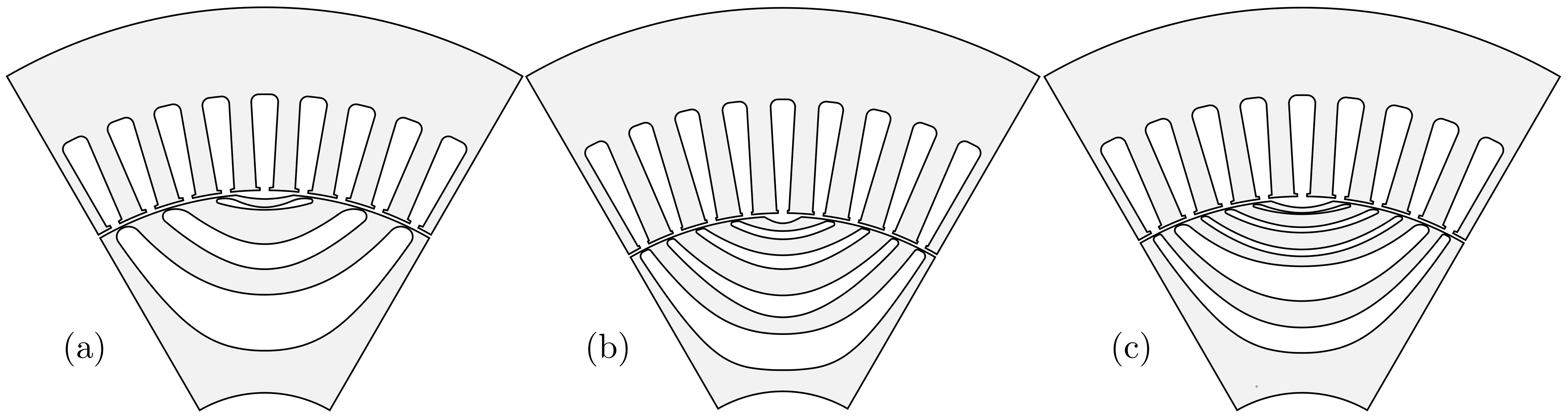
2. SyRM Rotor Barriers
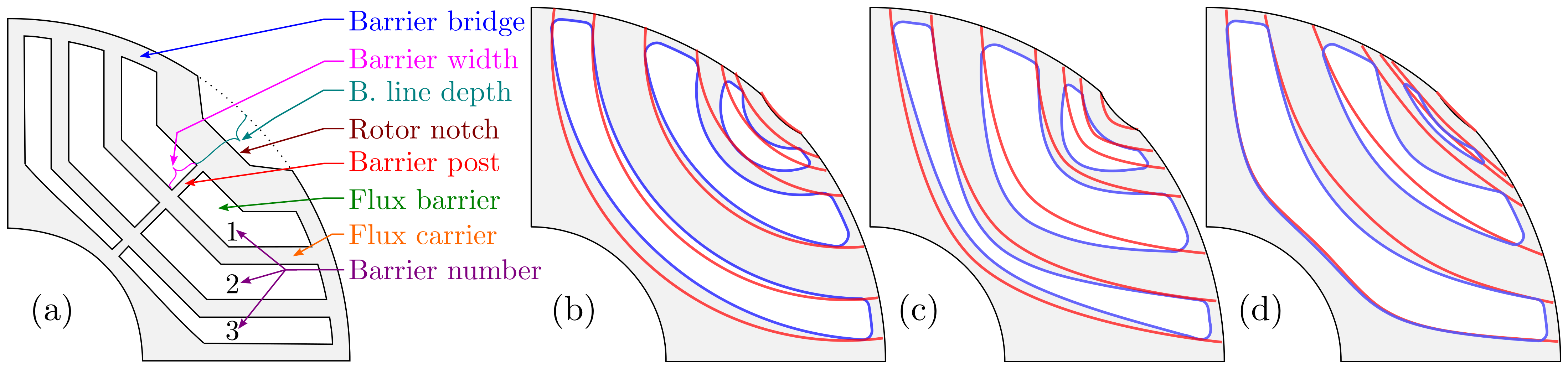
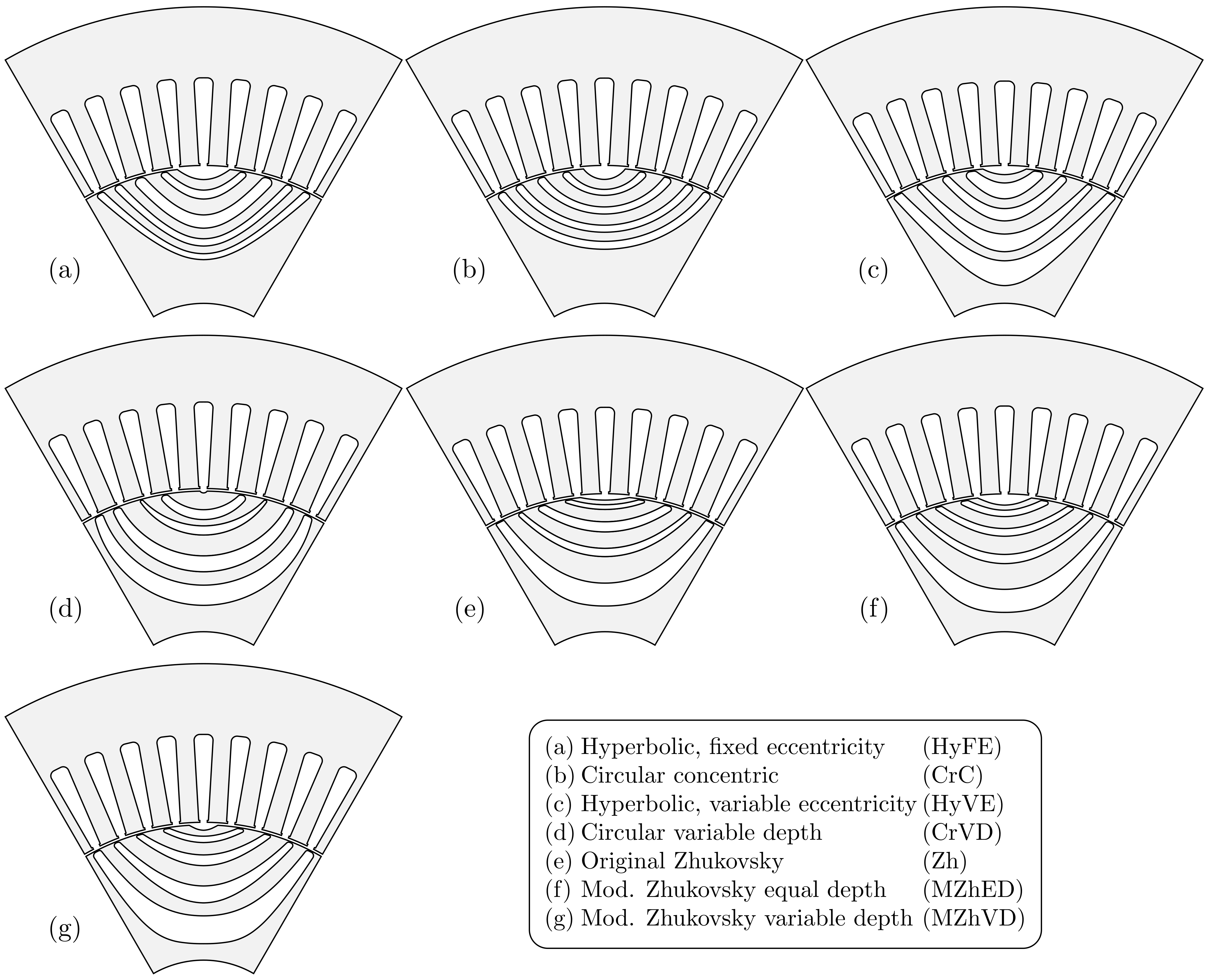
- Circular concentric (CrC), Figure 2b (red);
- Circular variable depth (CrVD), Figure 2b (blue);
- Hyperbolic, fixed eccentricity (HyFE), Figure 2c (red);
- Hyperbolic, variable eccentricity (HyVE), Figure 2c (blue);
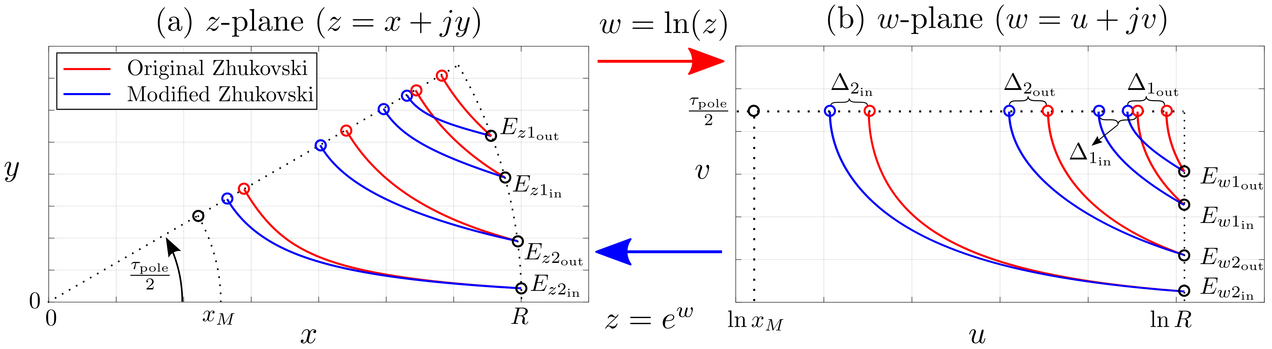
- Original Zhukovsky (Zh), Figure 2d (red);
- Modified Zhukovsky variable depth (MZhVD), Figure 2d (blue);
- Modified Zhukovsky with equal depth (MZhED, a special case of previous topology).
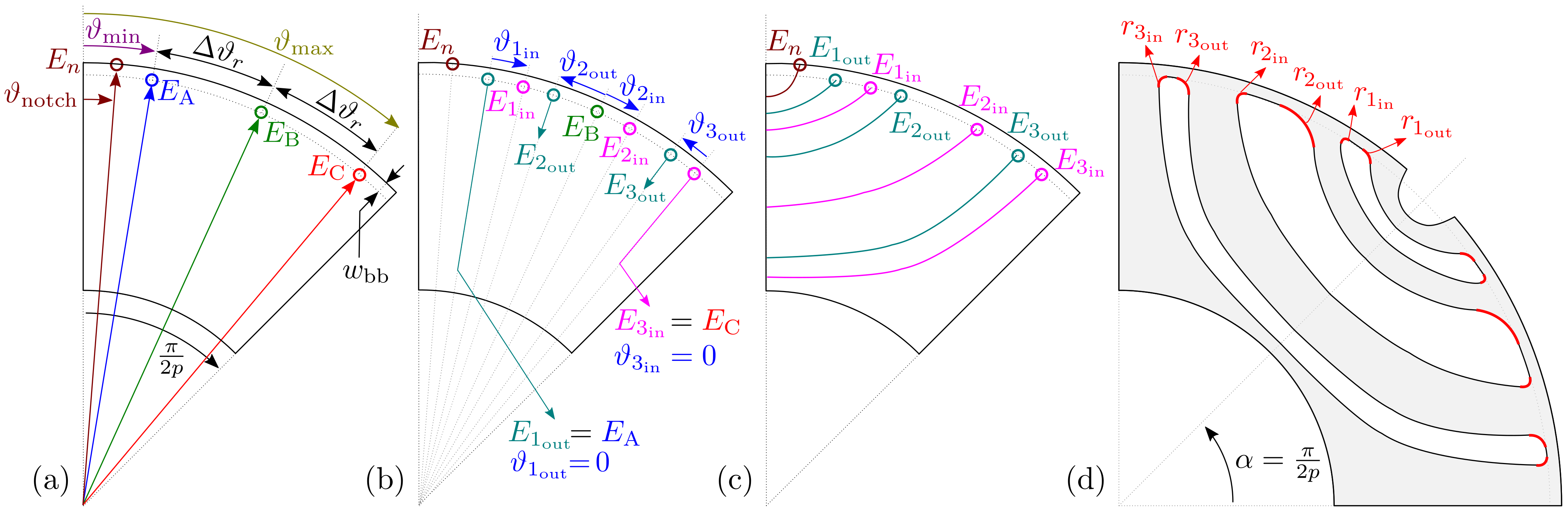
2.1. Automated Barrier Design
2.2. Barrier Depth Variation
2.3. Zhukovsky Barrier Modification
3. Optimization
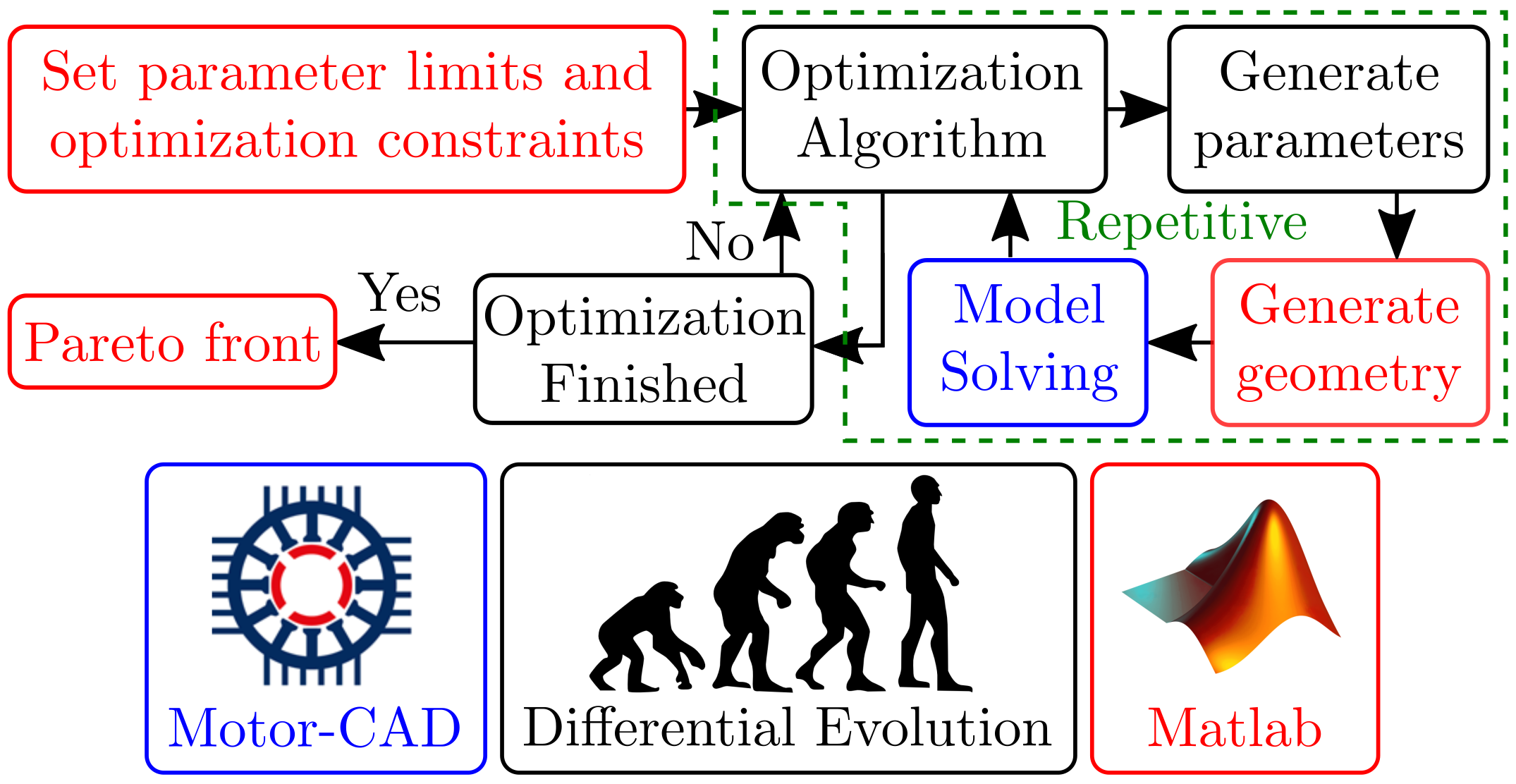
3.1. Typical Optimization pProcedure
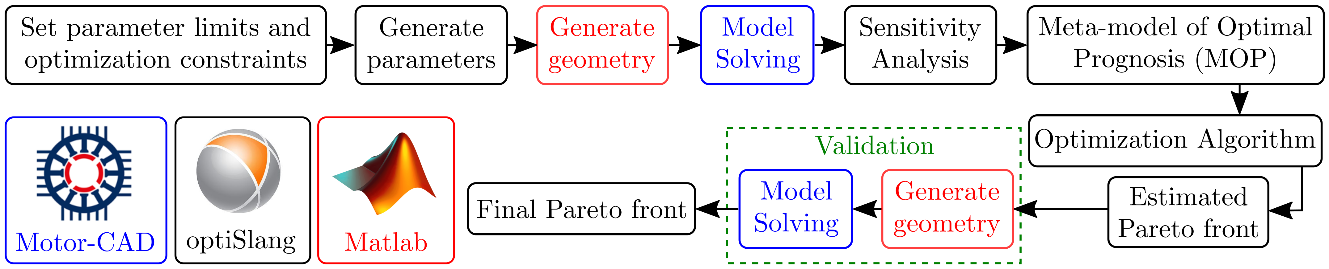
3.2. OptiSlang Optimization Details
- Instead of several thousands, OSL runs only FEA calls;
- Once sensitivity analysis is completed on , the user sets objectives, constraints and runs a fast GA optimization procedure ( FEA calls). In case some of the goals and constraints have to be modified, sensitivity analysis does not have to be repeated. The user only re-runs optimization and validates it on FEA calls. This is very handy for projects with fluid requirements (e.g., change of rated battery voltage, driving cycle, peak power requirement etc.);
- Thousands of designs can be evaluated through MOPs within minutes by the selected optimization algorithm;
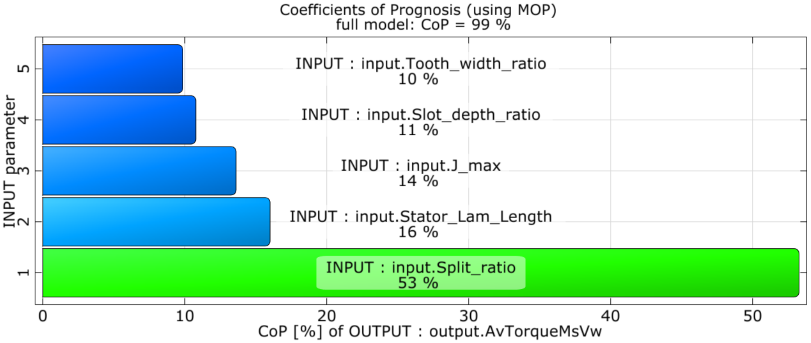
- Sensitivity analysis gives a valuable insight into where to concentrate the efforts for specified motor requirements [38].
3.3. Performance Requirements
3.4. Optimization Objectives and Inequality Constraints
3.5. Preset Model
4. Optimization Results
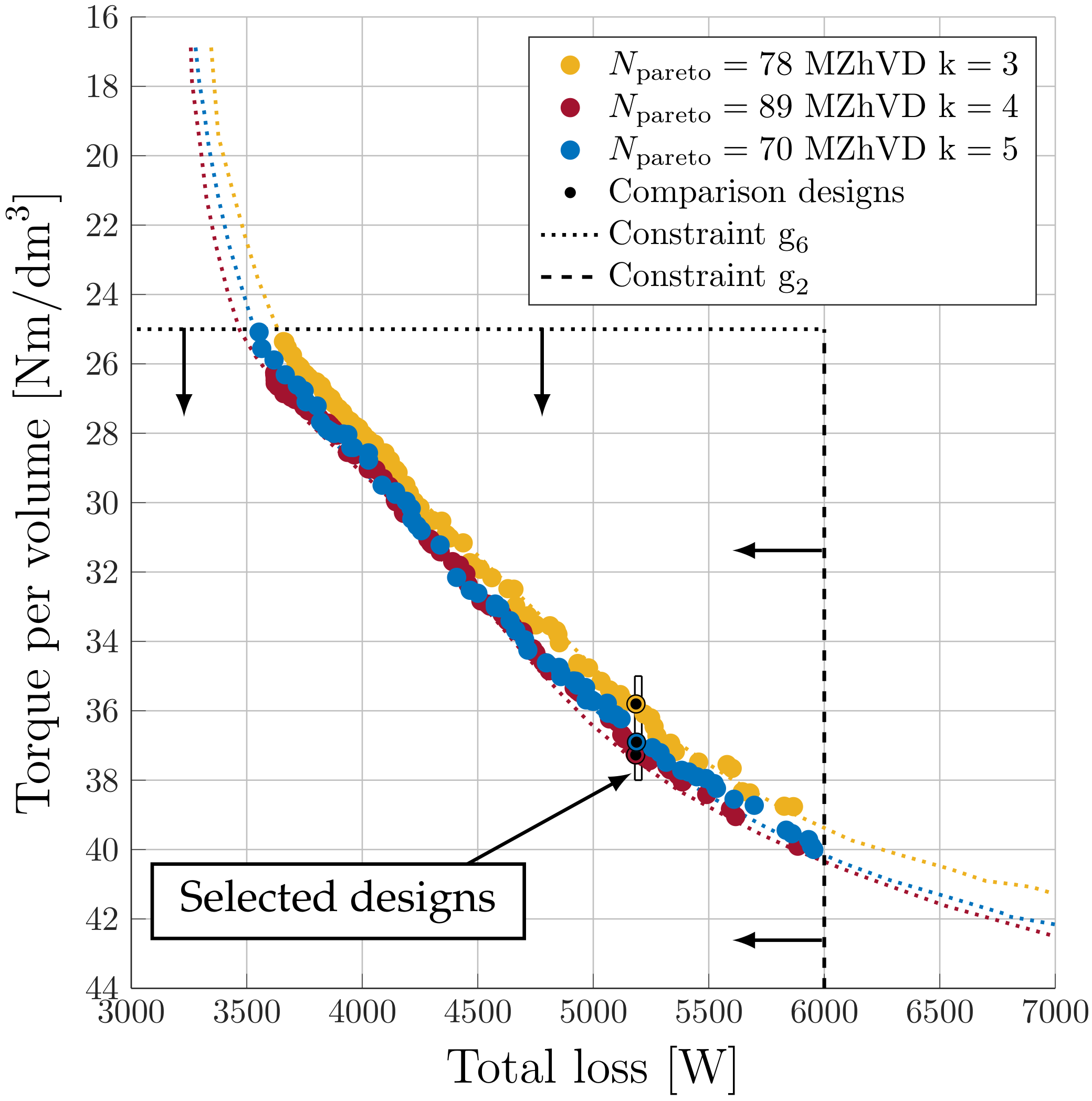
4.1. Rotor Topology Selection
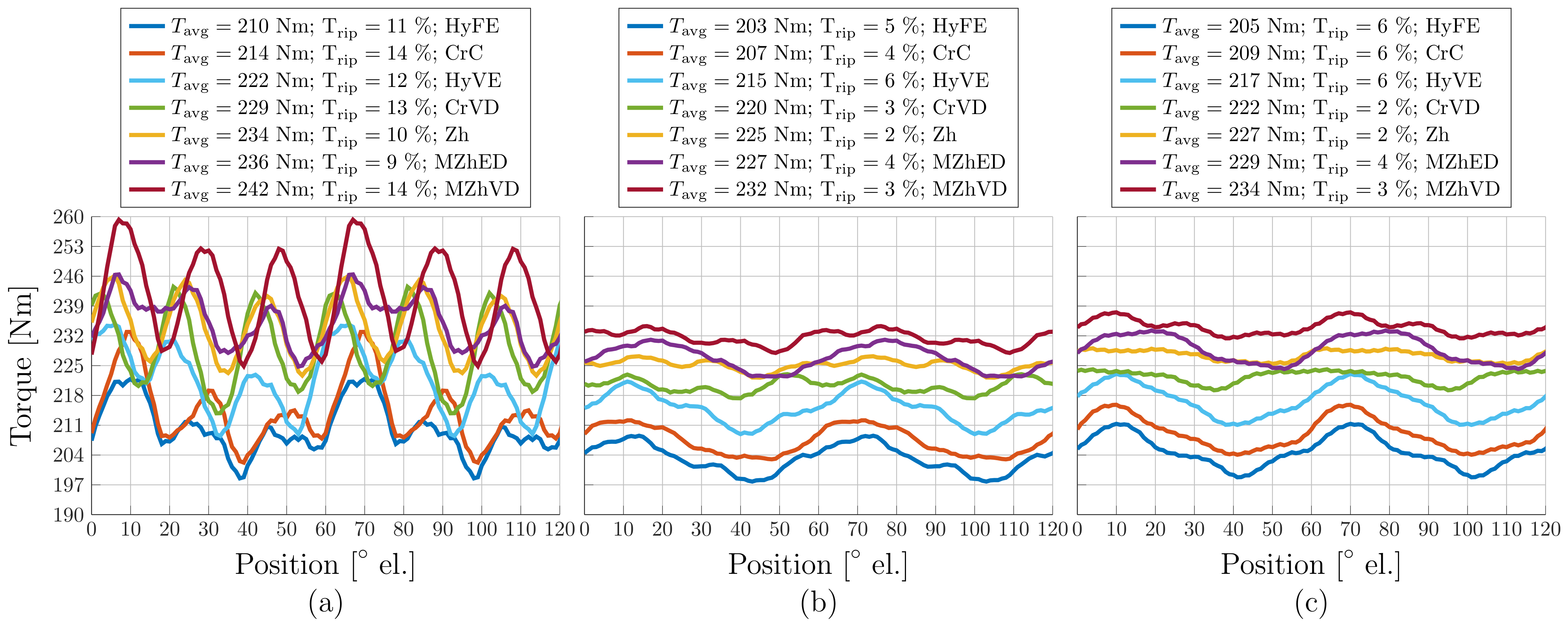
4.2. Torque Ripple Mitigation
4.3. Barrier Number Considerations
4.4. Execution Time and Computational Cost
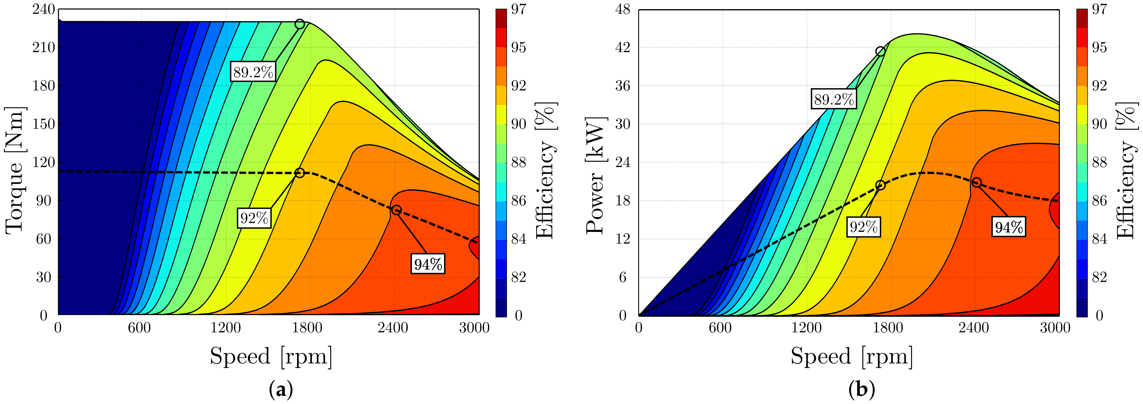
4.5. Efficiency Consideration
5. Conclusions
- Asymmetric rotor topologies with the purpose of torque ripple reduction without skewing.
- Torque ripple mitigation methods based on non-uniform rotor skew angles and variable segment lengths.
- Algorithm for the addition of precise corner fillets to arbitrary poly-line curves.
Author Contributions
Funding
Institutional Review Board Statement
Informed Consent Statement
Data Availability Statement
Acknowledgments
Conflicts of Interest
Abbreviations
| Abbreviation | Description |
| ASKA | Adaptive-Sampling Kriging Algorithm |
| CoP | Coefficient of prognosis |
| CPU | Central processing unit |
| CrC | Circular concentric barrier |
| CrVD | Circular variable depth barrier |
| DE | Differential evolution |
| e-PTO | Electric power take off |
| EV | Electric vehicle |
| FEA | Finite element analysis |
| GA | Genetic algorithm |
| HyFE | Hyperbolic fixed eccentricity barrier |
| HyVE | Hyperbolic variable eccentricity barrier |
| IM | Induction machine |
| IPM | Interior permanent magnet |
| MOP | Model of prognosis |
| MTPA | Maximum torque per Ampere |
| MZhED | Modified Zhukovsky equal depth barrier |
| MZhVD | Modified Zhukovsky variable depth barrier |
| NGnet | Normalized Gaussian network |
| OA | Optimization algorithm |
| OSL | OptiSlang |
| PM | Permanent magnet |
| PTO | Power take off |
| SyRM | Synchronous reluctance machine |
| TPV | Torque per volume |
| THL | Thermal loading coefficient |
| Zh | Original Zhukovsky barrier |
References
- Murataliyev, M.; Degano, M.; Nardo, M.D.; Bianchi, N.; Gerada, C. Synchronous Reluctance Machines: A Comprehensive Review and Technology Comparison. Proc. IEEE 2022, 110, 382–399. [Google Scholar] [CrossRef]
- Ban, B.; Stipetic, S.; Klanac, M. Synchronous reluctance machines: Theory, design and the potential Use in traction applications. In Proceedings of the International Conference on Electrical Drives and Power Electronics, High Tatras, Slovakia, 24–26 September 2019; pp. 177–188. [Google Scholar]
- Ban, B.; Stipetić, S. Electric Multipurpose Vehicle Power Take-Off: Overview, Load Cycles and Actuation via Synchronous Reluctance Machine. In Proceedings of the International Aegean Conference on Electrical Machines and Power Electronics (ACEMP-OPTIM), Istanbul, Turkey, 27–29 August 2019. [Google Scholar]
- Ban, B.; Stipetic, S. Design and optimization of synchronous reluctance machine for actuation of electric multi-purpose vehicle power take-off. In Proceedings of the 2020 International Conference on Electrical Machines, (ICEM 2020), Online, 23–26 March 2020; pp. 1750–1757. [Google Scholar]
- Lampinen, J. Multi-Constrained Nonlinear Optimization by the Differential Evolution Algorithm. In Soft Computing and Industry; Springer: London, UK, 2002. [Google Scholar]
- Zarko, D. A Systematic Approach to Optimized Design of Permanent Magnet Motors with Reduced Torque Pulsations. Ph.D. Thesis, University of Wisconsin, Madison, WI, USA, 2004. [Google Scholar]
- Stipetic, S.; Miebach, W.; Zarko, D. Optimization in design of electric machines: Methodology and workflow. In Proceedings of the Joint International Conference-ACEMP 2015: Aegean Conference on Electrical Machines and Power Electronics, OPTIM 2015: Optimization of Electrical and Electronic Equipment and ELECTROMOTION 2015: International Symposium on Advanced Electromechanical Moti, Side, Turkey, 2–4 September 2016; pp. 441–448. [Google Scholar]
- Gamba, M.; Pellegrino, G.; Armando, E.; Ferrari, S. Synchronous Reluctance Motor with Concentrated Windings for IE4 Efficiency. In Proceedings of the IEEE Energy Conversion Congress and Exposition (ECCE), Cincinnati, OH, USA, 1–5 October 2017. [Google Scholar]
- Calzo, G.L.; Galea, M. Design Optimization of a High-Speed Synchronous Reluctance Machine. IEEE Trans. Ind. Appl. 2018, 54, 233–243. [Google Scholar]
- Babetto, C.; Bacco, G.; Bianchi, N. Synchronous Reluctance Machine Optimization for High-Speed Applications. IEEE Trans. Energy Convers. 2018, 33, 1266–1273. [Google Scholar] [CrossRef]
- De Pancorbo, S.M.; Ugalde, G.; Poza, J.; Egea, A. Comparative study between induction motor and Synchronous Reluctance Motor for electrical railway traction applications. In Proceedings of the 5th International Conference on Electric Drives Production, (EDPC 2015), Nuremberg, Germany, 15–16 September 2015; pp. 2–6. [Google Scholar]
- Villan, M.; Tursini, M.; Popescu, M.; Fabri, G.; Credo, A.; Di Leonardo, L. Experimental comparison between induction and synchronous reluctance motor-drives. In Proceedings of the 2018 23rd International Conference on Electrical Machines, ICEM 2018, Alexandroupoli, Greece, 3–6 September 2018; pp. 1188–1194. [Google Scholar]
- Villani, M. High Performance Electrical Motors for Automotive Applications–Status and Future of Motors with Low Cost Permanent Magnets. Ph.D. Thesis, University of l’Aquila, Aquila, Italy, 2020. [Google Scholar]
- Castagnaro, E.; Bianchi, N. High-Speed Synchronous Reluctance Motor for Electric-Spindle Application; Institute of Electrical and Electronics Engineers Inc.: Piscataway, NJ, USA, 2020; pp. 2419–2425. [Google Scholar]
- Bao, Y.; Degano, M.; Wang, S.; Chuan, L.; Zhang, H.; Xu, Z.; Gerada, C. A Novel Concept of Ribless Synchronous Reluctance Motor for Enhanced Torque Capability. IEEE Trans. Ind. Electron. 2020, 67, 2553–2563. [Google Scholar] [CrossRef]
- Credo, A.; Fabri, G.; Villani, M.; Popescu, M. High speed synchronous reluctance motors for electric vehicles: A focus on rotor mechanical design. In Proceedings of the 2019 IEEE International Electric Machines and Drives Conference, (IEMDC 2019), San Diego, CA, USA, 12–15 May 2019; pp. 165–171. [Google Scholar]
- Kafadar, A.S.; Tap, A.; Ergene, L.T. Torque ripple reduction of SynRM using machaon type lamination. In Proceedings of the 2018 6th International Conference on Control Engineering and Information Technology, (CEIT 2018), Istanbul, Turkey, 25–27 October 2018; pp. 25–27. [Google Scholar]
- Ban, B.; Stipetic, S. Absolutely Feasible Synchronous Reluctance Machine Rotor Barrier Topologies with Minimal Parametric Complexity. Machines 2022, 10, 206. [Google Scholar] [CrossRef]
- Ferrari, M.; Bianchi, N.; Doria, A.; Fornasiero, E. Design of Synchronous Reluctance Motor for Hybrid Electric Vehicles. IEEE Trans. Ind. Appl. 2015, 51, 21–36. [Google Scholar] [CrossRef]
- Tawfiq, K.B.; Ibrahim, M.N.; El-Kholy, E.E.; Sergeant, P. Performance Improvement of Synchronous Reluctance Machines—A Review Research. IEEE Trans. Magn. 2021, 57, 99. [Google Scholar] [CrossRef]
- Varatharajan, A.; Brunelli, D.; Ferrari, S.; Pescetto, P.; Pellegrino, G. SyreDrive: Automated Sensorless Control Code Generation for Synchronous Reluctance Motor Drives; Institute of Electrical and Electronics Engineers Inc.: Piscataway, NJ, USA, 2021; pp. 192–197. [Google Scholar]
- Tawfiq, K.B.; Ibrahim, M.N.; El-Kholy, E.E.; Sergeant, P. Performance Analysis of a Rewound Multiphase Synchronous Reluctance Machine. IEEE J. Emerg. Sel. Top. Power Electron. 2022, 10, 297–309. [Google Scholar] [CrossRef]
- Tawfiq, K.B.; Ibrahim, M.N.; El-Kholy, E.E.; Sergeant, P. Construction of Synchronous Reluctance Machines with Combined Star-Pentagon Configuration Using Standard Three-Phase Stator Frames. IEEE Trans. Ind. Electron. 2022, 69, 7582–7595. [Google Scholar] [CrossRef]
- Ibrahim, M.N.F.; Abdel-Khalik, A.S.; Rashad, E.M.; Sergeant, P. An Improved Torque Density Synchronous Reluctance Machine with a Combined Star-Delta Winding Layout. IEEE Trans. Energy Convers. 2018, 33, 1015–1024. [Google Scholar] [CrossRef]
- Ibrahim, M.N.; Sergeant, P.; Rashad, E.M. Synchronous Reluctance Motor Performance Based on Different Electrical Steel Grades. IEEE Trans. Magn. 2015, 51, 7403304. [Google Scholar] [CrossRef]
- Mirazimi, M.S.; Kiyoumarsi, A. Magnetic Field Analysis of Multi-Flux-Barrier Interior Permanent-Magnet Motors Through Conformal Mapping. IEEE Trans. Magn. 2017, 53, 7002512. [Google Scholar] [CrossRef]
- Mirazimi, M.S.; Kiyoumarsi, A. Magnetic Field Analysis of SynRel and PMASynRel Machines with Hyperbolic Flux Barriers Using Conformal Mapping. IEEE Trans. Transp. Electrif. 2020, 6, 52–61. [Google Scholar] [CrossRef]
- Taghavi, S.; Pillay, P. Design aspects of a 50hp 6-pole synchronous reluctance motor for electrified powertrain applications. In Proceedings of the IECON 2017—43rd Annual Conference of the IEEE Industrial Electronics Society, Beijing, China, 29 October–1 November 2017; pp. 2252–2257. [Google Scholar]
- Gamba, M.; Pellegrino, G.; Cupertino, F. Optimal number of rotor parameters for the automatic design of Synchronous Reluctance machines. In Proceedings of the 2014 International Conference on Electrical Machines, ICEM 2014, Berlin, Germany, 9 February 2014; pp. 1334–1340. [Google Scholar]
- Cupertino, F.; Pellegrino, G.; Cagnetta, P.; Ferrari, S.; Perta, M. SyRE: Synchronous Reluctance (Machines)-Evolution. 2021. Available online: https://sourceforge.net/projects/syr-e/ (accessed on 15 August 2022).
- Kamper, M.J.; Van Der Merwe, F.S.; Williamson, S. Direct Finite Element Design Optimisation of the Cageless Reluctance Synchronous Machine. IEEE Trans. Energy Convers. 1996, 11, 547–553. [Google Scholar] [CrossRef]
- Gundogdu, T.; Komurgoz, G. A systematic design optimization approach for interior permanent magnet machines equipped with novel semi-overlapping windings. Struct. Multidiscip. Optim. 2021, 63, 1491–1512. [Google Scholar] [CrossRef]
- Lee, J.; Seo, J.H.; Kikuchi, N. Topology optimization of switched reluctance motors for the desired torque profile. Struct. Multidiscip. Optim. 2010, 42, 783–796. [Google Scholar] [CrossRef]
- Lee, C.; Jang, I.G. Topology optimization of multiple-barrier synchronous reluctance motors with initial random hollow circles. Struct. Multidiscip. Optim. 2021, 64, 2213–2224. [Google Scholar] [CrossRef]
- Otomo, Y.; Igarashi, H. Topology Optimization Using Gabor Filter: Application to Synchronous Reluctance Motor. IEEE Trans. Magn. 2021, 9464, 18–21. [Google Scholar] [CrossRef]
- Bramerdorfer, G.; Zǎvoianu, A.C. Surrogate-Based Multi-Objective Optimization of Electrical Machine Designs Facilitating Tolerance Analysis. IEEE Trans. Magn. 2017, 53, 1–11. [Google Scholar] [CrossRef]
- Son, J.c.; Ahn, J.m.; Lim, J. Optimal Design of PMa-SynRM for Electric Vehicles Exploiting Adaptive-Sampling Kriging Algorithm. IEEE Access 2021, 9, 41174–41183. [Google Scholar] [CrossRef]
- Riviere, N.; Volpe, G.; Villani, M.; Fabri, G.; Di Leonardo, L.; Popescu, M. Design analysis of a high speed copper rotor induction motor for a traction application. In Proceedings of the 2019 IEEE International Electric Machines and Drives Conference, (IEMDC 2019), San Diego, CA, USA, 12–15 May 2019. [Google Scholar]
- Stipetic, S.; Zarko, D.; Popescu, M. Ultra-fast axial and radial scaling of synchronous permanent magnet machines. IET Electr. Power Appl. 2016, 10, 658–666. [Google Scholar] [CrossRef]
- Bomela, X.B.; Kamper, M.J. Effect of stator chording and rotor skewing on performance of reluctance synchronous machine. IEEE Trans. Ind. Appl. 2002, 38, 91–100. [Google Scholar] [CrossRef]
- Hubert, T.; Reinlein, M.; Kremser, A.; Herzog, H.G. Torque ripple minimization of reluctance synchronous machines by continuous and discrete rotor skewing. In Proceedings of the 2015 5th International Conference on Electric Drives Production, (EDPC 2015), Nuremberg, Germany, 15–16 September 2015. [Google Scholar]
- Pellegrino, G. Permanent Magnet Machine Design and Analysis with a Focus to Flux-switching PM and PM-assisted Synchronous Reluctance Machines Part II: PM-assisted Synch Rel Machines Tutorials. In Proceedings of the 2016 International Conference on Electrical Machines, (ICEM 2016), Lausanne, Switzerland, 4–7 September 2016. [Google Scholar]
- Vagati, A.; Pastorelli, M.; Franceschini, G.; Petrache, S.C. Design of low-torque-ripple synchronous reluctance motors. IEEE Trans. Ind. Appl. 1998, 34, 758–765. [Google Scholar] [CrossRef]


| Description | Symbol | Value | Unit |
|---|---|---|---|
| Base speed | 1700 | rpm | |
| Max. operating speed | 2500 | rpm | |
| Max. torque | ≥200 | Nm | |
| Battery voltage | 610 | V | |
| Max. phase current | 300 | Arms |
| No: | Constraint Description | Symbol | Limit |
|---|---|---|---|
| Stress yield factor at | FOS | ≥2 | |
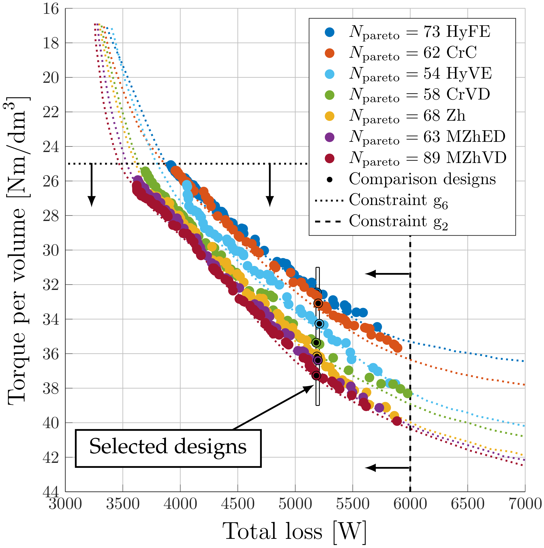
| Total loss | ≤6000 W | ||
| Flux density in stator yoke | ≤1.6 T | ||
| Flux density in stator tooth | ≤1.9 T | ||
| Thermal loading | THL | ≤1.9 MA2/m3 | |
| Torque per volume | TPV | ≥25 Nm/dm3 | |
| Torque ripple without skewing | ≤15% | ||
| No: | Optimization Goals | Symbol | Unit |
| Minimize total loss | W | ||
| Maximize torque per rotor volume | TPV | Nm/dm3 |
| No: | Description | Symbol | Value/Range | Unit |
|---|---|---|---|---|
| 1 | Stator diameter | 214 | mm | |
| 2 | Shaft diameter | 54 | mm | |
| 3 | Phase number | 3 | - | |
| 4 | No. of turns | Automatic | - | |
| 5 | Parallel paths | Automatic | - | |
| 6 | Coil throw | 9 | - | |
| 7 | Barrier number | k | 4 | - |
| 8 | Pole pairs | p | 3 | - |
| 9 | Slot number | 54 | - | |
| 10 | Barrier bridge | 0.3 | mm | |
| 11 | Airgap | 0.7 | mm | |
| 12 | Slot opening | 2 | mm | |
| 13 | Fill factor | - | 0.43 | - |
| 14 | Tooth tip depth | 0.5 | mm |
| No: | Description | Symbol | Value/Range | Unit |
|---|---|---|---|---|
| 15 | Point1 inner angle | - | ||
| 16 | Point1 outer angle | 0 | - | |
| 17 | Point2 inner angle | - | ||
| 18 | Point2 outer angle | - | ||
| 19 | Point3 inner angle | - | ||
| 20 | Point3 outer angle | - | ||
| 21 | Point4 inner angle | 0 | - | |
| 22 | Point4 outer angle | - | ||
| 23–26 | Corner radius in | - | ||
| 27–30 | Corner radius out | - | ||
| 31 | Slot corner radius | - | ||
| 32 | Slot depth ratio | - | ||
| 33 | Split ratio | - | ||
| 34 | Active length | mm | ||
| 35 | Tooth tip angle | ∘ | ||
| 36 | Tooth width ratio | - | ||
| 37 | Min. angle | - | ||
| 38 | Max. angle | - | ||
| 39 | Notch angle | - | ||
| 40 | Current density | J | A/mm2 | |
| 41–44 | Barrier depths | - | ||
| 45–48 | Barrier depths | - | ||
| 49 | Notch depth | - |
| Name | Unit | HyFE | CrC | HyVE | CrVD | Zh | MZhED | MZhVD |
|---|---|---|---|---|---|---|---|---|
| TPV | Nm/dm3 | 32.5 | 33.1 | 34.3 | 35.4 | 36.2 | 36.4 | 37.3 |
| dm3 | 6.47 | 6.47 | 6.47 | 6.47 | 6.47 | 6.47 | 6.47 | |
| kW | 5188 | 5199 | 5209 | 5182 | 5188 | 5197 | 5184 | |
| kW | 37.4 | 38.1 | 39.5 | 40.8 | 41.7 | 41.9 | 43.0 | |
| Nm | 210.1 | 214.2 | 221.9 | 229.0 | 234.1 | 235.6 | 241.3 | |
| % | 12.1 | 14.1 | 11.7 | 12.7 | 9.7 | 9.3 | 13.7 | |
| n | rpm | 1700 | 1700 | 1700 | 1700 | 1700 | 1700 | 1700 |
| T | 1.53 | 1.53 | 1.39 | 1.60 | 1.52 | 1.54 | 1.56 | |
| T | 1.86 | 1.87 | 1.87 | 1.82 | 1.87 | 1.86 | 1.84 | |
| FOS | - | 8.8 | 9.4 | 7.3 | 6.3 | 3.6 | 5.2 | 6.3 |
| m | kg | 45.6 | 46.0 | 44.2 | 44.3 | 45.0 | 44.8 | 44.1 |
| THL | MA2/m3 | 1.52 | 1.53 | 1.57 | 1.47 | 1.53 | 1.52 | 1.52 |
| mm | 180 | 180 | 180 | 180 | 180 | 180 | 180 | |
| ∘ | 57.9 | 60.3 | 61.4 | 62.5 | 61.8 | 61.8 | 62.9 | |
| Arms | 95.6 | 95.6 | 94.3 | 94.1 | 95.9 | 95.7 | 95.7 | |
| - | 0.61 | 0.62 | 0.66 | 0.67 | 0.67 | 0.67 | 0.69 | |
| % | 87.8 | 88.0 | 88.3 | 88.7 | 88.9 | 89.0 | 89.2 | |
| Gain | % | 0.0 | 1.9 | 5.6 | 9.0 | 11.4 | 12.1 | 14.9 |
| No: | Description | Symbol | Zh | MZhED | HyFE | CrC | MZhVD | HyVE | CrVD | Unit |
|---|---|---|---|---|---|---|---|---|---|---|
| 1 | Stator diameter | 214 | 214 | 214 | 214 | 214 | 214 | 214 | mm | |
| 2 | Shaft diameter | 54 | 54 | 54 | 54 | 54 | 54 | 54 | mm | |
| 3 | Phase number | 3 | 3 | 3 | 3 | 3 | 3 | 3 | - | |
| 4 | No. of turns | 21 | 21 | 21 | 21 | 22 | 21 | 21 | - | |
| 5 | Parallel paths | 6 | 6 | 6 | 6 | 6 | 6 | 6 | - | |
| 6 | Coil throw | 9 | 9 | 9 | 9 | 9 | 9 | 9 | - | |
| 7 | Barrier number | k | 4 | 4 | 4 | 4 | 4 | 4 | 4 | - |
| 8 | Pole pairs | p | 3 | 3 | 3 | 3 | 3 | 3 | 3 | - |
| 9 | Slot number | 54 | 54 | 54 | 54 | 54 | 54 | 54 | - | |
| 10 | Barrier bridge | 0.3 | 0.3 | 0.3 | 0.3 | 0.3 | 0.3 | 0.3 | mm | |
| 11 | Airgap | 0.7 | 0.7 | 0.7 | 0.7 | 0.7 | 0.7 | 0.7 | mm | |
| 12 | Slot opening | 2 | 2 | 2 | 2 | 2 | 2 | 2 | mm | |
| 13 | Fill factor | - | 0.43 | 0.43 | 0.43 | 0.43 | 0.43 | 0.43 | 0.43 | - |
| 14 | Tooth tip depth | 0.5 | 0.5 | 0.5 | 0.5 | 0.5 | 0.5 | 0.5 | mm | |
| 15 | Point1 inner angle | 0.35 | 0.42 | 0.35 | 0.35 | 0.35 | 0.35 | 0.46 | - | |
| 16 | Point1 outer angle | 0.00 | 0.00 | 0.00 | 0.00 | 0.00 | 0.00 | 0.00 | - | |
| 17 | Point2 inner angle | 0.40 | 0.33 | 0.46 | 0.36 | 0.29 | 0.12 | 0.25 | - | |
| 18 | Point2 outer angle | 0.00 | -0.04 | 0.06 | 0.01 | 0.00 | 0.00 | 0.06 | - | |
| 19 | Point3 inner angle | 0.12 | 0.13 | 0.25 | 0.24 | 0.18 | 0.24 | 0.14 | - | |
| 20 | Point3 outer angle | 0.09 | 0.09 | 0.09 | 0.09 | 0.09 | 0.09 | 0.09 | - | |
| 21 | Point4 inner angle | 0.00 | 0.00 | 0.00 | 0.00 | 0.00 | 0.00 | 0.00 | - | |
| 22 | Point4 outer angle | 0.35 | 0.35 | 0.35 | 0.35 | 0.35 | 0.35 | 0.35 | - | |
| 23 | Corner radius1 inner | 0.89 | 0.90 | 0.94 | 0.90 | 0.91 | 0.90 | 0.89 | - | |
| 24 | Corner radius1 outer | 0.90 | 0.90 | 0.89 | 0.88 | 0.89 | 0.90 | 0.91 | - | |
| 25 | Corner radius2 inner | 0.88 | 0.16 | 0.90 | 0.90 | 0.50 | 0.90 | 0.90 | - | |
| 26 | Corner radius2 outer | 0.87 | 0.90 | 0.90 | 0.55 | 0.90 | 0.99 | 0.90 | - | |
| 27 | Corner radius3 inner | 0.88 | 0.89 | 0.90 | 0.89 | 0.90 | 0.88 | 0.89 | - | |
| 28 | Corner radius3 outer | 0.90 | 0.90 | 0.90 | 0.90 | 0.90 | 0.90 | 0.90 | - | |
| 29 | Corner radius4 inner | 0.02 | 0.85 | 0.73 | 0.99 | 0.95 | 0.89 | 0.49 | - | |
| 30 | Corner radius4 outer | 0.20 | 0.77 | 0.74 | 0.85 | 0.63 | 0.54 | 0.20 | - | |
| 31 | Slot corner radius | 0.62 | 0,61 | 0.63 | 0.62 | 0.59 | 0.61 | 0.63 | - | |
| 32 | Slot depth ratio | 0.48 | 0.45 | 0.46 | 0.50 | 0.46 | 0.46 | 0.46 | - | |
| 33 | Split ratio | 0.67 | 0.72 | 0.61 | 0.72 | 0.67 | 0.66 | 0.61 | - | |
| 34 | Active length | 180 | 180 | 180 | 180 | 180 | 180 | 180 | mm | |
| 35 | Tooth tip angle | 9.45 | 9.48 | 9.49 | 9.50 | 9.48 | 9.47 | 9.49 | ∘ | |
| 36 | Tooth width ratio | 0.88 | 0.82 | 0.78 | 0.87 | 0.71 | 0.84 | 0.78 | - | |
| 37 | Min. angle | 0.14 | 0.16 | 0.16 | 0.15 | 0.15 | 0.15 | 0.12 | - | |
| 38 | Max. angle | 0.48 | 0.49 | 0.48 | 0.48 | 0.50 | 0.47 | 0.50 | - | |
| 39 | Notch angle | 0.72 | 0.73 | 0.71 | 0.59 | 0.42 | 0.10 | 0.75 | - | |
| 40 | Current density | J | 17 | 17 | 17 | 17 | 17 | 17 | 17 | A/mm2 |
| 41 | Barrier depth1 | - | 0.90 | 0.67 | 0.80 | 0.70 | 0.40 | 0.40 | - | |
| 42 | Barrier depth2 | - | 0.90 | 0.67 | 0.80 | 0.48 | 0.59 | 0.39 | - | |
| 43 | Barrier depth3 | - | 0.90 | 0.67 | 0.80 | 0.48 | 0.43 | 0.42 | - | |
| 44 | Barrier depth4 | - | 0.90 | 0.67 | 0.80 | 0.71 | 0.60 | 0.63 | - | |
| 45 | Barrier depth1 | - | 0.90 | 0.67 | 0.80 | 0.80 | 0.40 | 0.64 | - | |
| 46 | Barrier depth2 | - | 0.90 | 0.67 | 0.80 | 0.81 | 0.53 | 0.79 | - | |
| 47 | Barrier depth3 | - | 0.90 | 0.67 | 0.80 | 0.79 | 0.68 | 0.79 | - | |
| 48 | Barrier depth4 | - | 0.90 | 0.67 | 0.80 | 0.92 | 0.80 | 0.42 | - | |
| 49 | Notch depth | - | 0.90 | 0.67 | 0.80 | 0.60 | 0.50 | 0.50 | - |
| Name | Unit | |||
|---|---|---|---|---|
| TPV | Nm/dm3 | 35.8 | 37.3 | 36.9 |
| dm3 | 6.47 | 6.47 | 6.47 | |
| kW | 5184.84 | 5184 | 5187 | |
| kW | 41.3 | 43.0 | 42.5 | |
| Nm | 231.8 | 241.3 | 238.9 | |
| % | 15.3 | 13.7 | 13.2 | |
| n | rpm | 1700 | 1700 | 1700 |
| T | 1.59 | 1.56 | 1.56 | |
| T | 1.87 | 1.84 | 1.83 | |
| FOS | - | 2.6 | 6.3 | 2.0 |
| m | kg | 43.2 | 44.1 | 44.0 |
| THL | MA2/m3 | 1.43 | 1.52 | 1.45 |
| mm | 180 | 180 | 180 | |
| ∘ | 62.2 | 62.9 | 63.2 | |
| Arms | 89.7 | 95.7 | 91.5 | |
| - | 0.70 | 0.69 | 0.70 | |
| % | 88.8 | 89.2 | 89.1 | |
| Gain | % | 0.0 | 4.1 | 3.1 |
| Stage | Avg. Design Eval. Time | Sensitivity Analysis | MOP Building | OSL Optimization | Pareto Validation | Total Execution Time | Total Execution Time | |
|---|---|---|---|---|---|---|---|---|
| Type | [s] | [min] | [min] | [min] | [min] | [min] | [h] | |
| Zh | 4 | 55.02 | 114.6 | 211.0 | 11.7 | 45.9 | 383.2 | 6.39 |
| MZhED | 4 | 55.60 | 115.8 | 218.9 | 12.2 | 46.3 | 393.2 | 6.55 |
| MZhVD | 3 | 55.89 | 116.4 | 232.0 | 12.9 | 46.6 | 407.9 | 6.80 |
| HyFE | 4 | 56.30 | 117.3 | 249.8 | 13.9 | 46.9 | 427.9 | 7.13 |
| CrC | 4 | 57.20 | 119.2 | 248.5 | 13.8 | 47.7 | 429.1 | 7.15 |
| MZhVD | 4 | 58.30 | 121.5 | 246.6 | 13.7 | 48.6 | 430.3 | 7.17 |
| HyVE | 4 | 58.20 | 121.3 | 248.6 | 13.8 | 48.5 | 432.2 | 7.20 |
| CrVD | 4 | 58.40 | 121.7 | 249.4 | 13.9 | 48.7 | 433.6 | 7.23 |
| MZhVD | 5 | 60.50 | 126.0 | 261.2 | 14.5 | 50.4 | 452.2 | 7.54 |
Publisher’s Note: MDPI stays neutral with regard to jurisdictional claims in published maps and institutional affiliations. |
© 2022 by the authors. Licensee MDPI, Basel, Switzerland. This article is an open access article distributed under the terms and conditions of the Creative Commons Attribution (CC BY) license (https://creativecommons.org/licenses/by/4.0/).
Share and Cite
Ban, B.; Stipetic, S. Systematic Metamodel-Based Optimization Study of Synchronous Reluctance Machine Rotor Barrier Topologies. Machines 2022, 10, 712. https://doi.org/10.3390/machines10080712
Ban B, Stipetic S. Systematic Metamodel-Based Optimization Study of Synchronous Reluctance Machine Rotor Barrier Topologies. Machines. 2022; 10(8):712. https://doi.org/10.3390/machines10080712
Chicago/Turabian StyleBan, Branko, and Stjepan Stipetic. 2022. "Systematic Metamodel-Based Optimization Study of Synchronous Reluctance Machine Rotor Barrier Topologies" Machines 10, no. 8: 712. https://doi.org/10.3390/machines10080712