Article

Stewart Platform Motion Control Automation with Industrial Resources to Perform Cycloidal and Oceanic Wave Trajectories

Automation and System Engineering Department, School of Industrial Engineering, Campus As Lagoas-Marcosende, Universidade de Vigo, 36310 Vigo, Spain
*
Author to whom correspondence should be addressed.
Machines 2022, 10(8), 711; https://doi.org/10.3390/machines10080711
Submission received: 18 July 2022 / Revised: 15 August 2022 / Accepted: 18 August 2022 / Published: 19 August 2022
(This article belongs to the Special Issue Development and Applications of Parallel Robots)

Abstract

:
Research on motion control automation of Stewart Platforms with industrial configurations (motion and controllers) is less present in the literature than other types of automation with low-cost devices such as Arduino, or via simulations in MATLAB or Simulink. Moreover, direct kinematics is less widely applied because of heavy calculation in real-time device implementations. The paper first analyzes the design, kinematic modelling, and trajectory generation of a Stewart Platform robot and addresses direct kinematics and motion automation. Next, the automation architecture with industrial controllers is detailed. The paper presents the results of the inverse kinematic in two use scenarios: cycloidal trajectories that carry out point-to-point and oceanic wave movements. The efficient calculation of direct kinematics in real time was also studied. This opens the possibility of closing the positioning loop at the controller or implementing supervisors such as the “tracking error”. Further research might investigate the effects of the sequence planning to avoid collisions with objects inside the workspace while considering the feedback of the tracking error.

1. Introduction

Parallel robots are composed of one or more closed kinematic chains that communicate their end effector (the tool) with the joints that provide the motion. These parallel robots are advantageous over serial robots because they generally have, among other characteristics, higher accelerations, a large load-to-weight ratio, higher motion accuracies to execute a task, high force capabilities because the output force is provided by multiple actuators working in parallel, as well as structures without bending loads [1,2,3].
The Stewart Platform is one of the most widely known parallel robots. This type of mechanism was presented by Stewart in [4], mainly to carry out flight simulations. In that research, Stewart focused on achieving, in the simplest way, a platform with six degrees of freedom in its motion. This platform used a maximum of six motors, and each motor had to work directly with the same load, thus obtaining a high ratio of the moving load to the weight of the structure. Due to the nature of the mechanism proposed by Stewart, this is considered a mixed parallel structure robot, which is a manipulator composed of a fixed base and a moving platform through two or more closed kinematic chains (six, in the particular case of the Stewart Platform) and with the capability of performing translational and spherical movements. Later, Hunt added in [5] that the platform would be useful as a manipulator in the context of robotics, which led many researchers to start their own field work with this type of mechanism. The first, McCallion, generalized the modifications and transformed the original concept into a more popular architecture [6]. This generalized Stewart Platform architecture is based on the use of two rigid bodies (base and mobile), which are connected by six extensible members with spherical joints at their lower and upper ends or with a universal joint at one end and a spherical joint at the other [6].
According to [7], there are 34 different possible configurations of the Stewart Platform in which the most common are 3-3, 6-3, and 6-6. The 3-3 configuration corresponds to a base and a mobile platform, both geometrically triangular, with two actuators placed at each vertex and with concentric joints. Examples of the use of such configurations were studied in [8,9]. The 6-3 configuration consists of a base platform with a hexagonal shape (it can be regular or irregular according to [10]) and a moving platform of triangular shape, with the actuators placed geometrically—two at each vertex of the moving platform and one at each vertex of the base. Examples of these configurations were studied in [11,12,13]. Finally, the 6-6 configuration corresponds to two hexagonal platforms (base and mobile), which may be irregular or regular hexagons, with the actuators arranged one by one at each vertex of the platform. Examples of this configuration can be found in [14,15,16].
Multiple combinations of joints in a Stewart Platform leg make various kinematic chain structures possible, as long as the platform can move and rotate on all three coordinate axes. When each member has a universal joint, followed by a prismatic joint and then a spherical joint, it is called UPS (Universal-Prismatic-Spherical), which is one of the most common distributions [17,18,19,20]. Another very common configuration is defined by a spherical joint at each end that is joined by a prismatic joint; this is called SPS (Spherical-Prismatic-Spherical). This SPS configuration, in contrast to the UPS, adds six passive degrees of freedom that allow for the rotation of the kinematic chain about its axis [21,22]. Some research studied a 6-UPU (Universal-Prismatic-Universal) Stewart Platform, where an actuator is connected to the moving platform and the base by two universal joints [23]. Another configuration is the UCU (Universal-Cylindrical-Universal) configuration, which achieves the six degrees of freedom from the possibility of rotation given by the cylindrical pair, as reported in [24]. Finally, there are also studies of Stewart Platforms that have flexible joints with no friction but with a gap, lubrication, and fast response, although these studies focused more on design, modelling, and simulation rather than on implementation [25,26].
The above configurations are very important for the kinematic study of the Stewart Platform since the kinematics strongly depends on the geometric design of the platform [27]. Kinematics focuses on the study of the movement of a mechanism with respect to a reference system, only taking into account its geometry and not the forces that may act on it. This study of kinematics can be divided into direct kinematics and inverse kinematics. Direct kinematics focuses on determining the position and orientation of the terminal element with respect to a reference system, given that the values of the joints and the geometry are known. Inverse kinematics, on the other hand, presents a joint configuration solution for a given position and orientation of the end element.
For this type of parallel manipulator, inverse kinematics is computationally easier than direct kinematics, as stated in [28]. Indeed, inverse kinematics has been implemented in most research about Stewart Platforms. In the literature, solutions to inverse kinematics have been given in detail, either expressed by the analytical loop equations [29,30,31,32], based on homogeneous coordinate transformation [33,34], or using the theory of screws [35,36].
Multiple researchers have also focused on the study of direct kinematics from different points of view: the authors of [28] presented the first attribution of the equations of the direct kinematics of the Stewart Platform with an SPS configuration. Fichter provided a solution to this problem using the Screw theory [29]. In [37], the closed analysis was based on the use of geometry in order to simplify the calculations. Other researchers focused their analysis on the use of Soma coordinates [21]. Due to the non-linearity of the series of simultaneous equations to be solved (and up to 40 possible configurations that the Stewart Platform can take [38]), Bonev [39] recommended the use of sensors to reduce the overdetermined system. Yee and Lim proposed the use of neural networks to obtain a direct solution [40], although iterative methods such as the Newton–Raphson method (and its modifications) have become the most widely used [41,42,43]. More recently, several researchers have started working on the calculation of direct kinematics with the use of new methods; e.g., [44] addressed the study of direct kinematics by vector regression, [45] provided a solution using the quaternions and Denavit–Hartenberg methods, and [7] showed a simplification for most of the configurations using virtual members and trilateration.
The use of Stewart Platforms extends to multiple applications: machine tools [46], architectural structures [47], rehabilitation processes [48], flight simulators [49], inspection [43], vibration isolation [20], driving simulator and stabilizers [50], high-precision positioning devices [51], micromanipulator applications [52], 3D printing [32], and for various applications in the marine oceanic area. One such application that is common in the maritime domain focuses on the use of Stewart Platforms to create an effective compensation of sea waves during the operation of a machine, such as cranes and drilling platforms [53,54]. Other examples that use of this type of platform are the floating offshore oceanic structures, as studied in [55,56], or in wave energy converters, which perform the motion of a particle under the free surface of the ocean [57]. As an ocean motion generator, [58] used a simulator composed of a boat model placed on the sea in order to recreate real ship motions and a Stewart Platform kept in a room in order to reproduce the motion.
Its real-time implementation with industrial axes, electric servomotors, and industrial controllers has been less studied in the literature than other types of implementations with low-cost devices such as Raspberry and Arduino, or simulations in MATLAB, Simulink, SimMechanics, ADAMS, etc. [13,59,60,61,62,63]. Furthermore, the implementation of inverse kinematics in this type of device is more studied than the implementation of direct kinematics, which has been scarcely studied. The use of industrial controllers is also driven, among other things, by the need for fine positioning and the synchronous operation of all linear actuators to achieve high accuracy in applications with Stewart Platforms [64].
Depending on the hardware structure of the control system, some implementations are employed with MATLAB running on a personal or industrial computer in order to perform some calculations and send axis commands to a specific motor control board. Rosell [65] studied control techniques based on real-time vision using MATLAB and Labview on a computer with a motor control board called the “Phidget AdvancedServo”. Lou and Tseng [66] focused on the transmission of positioning commands to a Stewart Platform using a common personal computer (Windows OS) with a servo motion control board as the controller. The authors developed a networked motion control system to guarantee the use of synchronous control and motion commands in the industrial linear motors. Shao [2] investigated the dynamics verification of a Stewart Platform by using an industrial PC with a Linux kernel to perform inverse and direct kinematic computations (MATLAB) and a multi-axis motor control board to send PWM signals to the servomotors.
Industrial controller devices can be seen as programmable logic controller (PLC) devices with numerical control capabilities that can manage the motion control of a set of axes. For example, the PLCopen Motion Control standard defines an automation framework based on standard Function Blocks in order to implement the movement of axes, thus enabling the numerical controller to generate the control sequences for interpolated movements [19]. Such machinery can be much smarter and more flexible because online recalculations can generate individual toolpaths as a process takes place instead of completing classic pre-defined trajectories.
Among the studies in the literature involving PLCs and industrial controllers, the following stand out. Walica and Noskievič [64] employed an industrial controller to control a simulated Stewart Platform in a real-time target in the dSPACE MicroLabBox. They used a PLCnext controller with the inverse kinematic and a proportional feedback controller automatically generated by the PLC Coder in Simulink. With this implementation, the code acted as a black box, and it could not be investigated or modified. He and Wen [67] investigated active disturbance rejection control techniques using a Stewart Platform with industrial servomotors, EtherCAT communications, and real-time control with TwinCAT. For this purpose, they only implemented the inverse kinematic without going into the details of the implementation. An and Huang [68] developed a sea wave surge base alignment test system, stressing the use of industrial controllers and industrial communication standards, such as EtherCAT, to improve the positioning of the platform. The control software was implemented in a C++ application in an industrial control computer. Porath [69] addressed a new kinematic calibration technique for Stewart Platforms using a PC as the controller, which had a real-time control application that had been developed in TwinCAT to perform the calculations of the inverse kinematics and to obtain pose data from a workstation server connected by WIFI with the industrial controller. Su [70] used industrial servomotors, although the control was performed on an industrial computer programmed in C, where inverse kinematics and friction compensation with a control period of 10 ms was implemented. Ordoñez and Rodriguez [71] addressed the implementation of a dynamic PID control in a Stewart Platform using xPC Target (a Matlab toolbox), with a user interface in the Simulink and Yaskawa industrial servomotors. Ming-Yen Wei [72] investigated inverse Kinematics and a monitoring system with the use of Labview on an industrial computer, which was responsible for processing all the sensors and sending the control information to the motors, and a PMDK motion control card, which was responsible for performing the tasks of motion, inverse kinematics, and for sending the motion pulses to the motors, although without going into implementation detail. Budaklı and Yılmaz [73] used MATLAB to run inverse and direct kinematics, providing the PID control and sending the tracking positions of the trajectory of each piston to the industrial controller. To do so, EtherCAT communication over the target processor in a real-time control system was employed. The target processor acted as the master of all six controllers.
However, considering the studies mentioned above, there is scarce research that used a control automation strategy without employing third-party environments (e.g., MATLAB, Simulink, ADAMS, etc.) to carry out calculations and control. That is, those that only used industrial controllers to calculate kinematics and drive motion on Stewart Platforms. Such a strategy would test the hypothesis that direct kinematics could be implemented efficiently with industrial controllers in a real-time environment. This would open the possibility of closing the positioning loop on the controller side. Hence, our motivation for undertaking this research is to test how 3D printers’ behavior is affected by ocean conditions. A Stewart Platform will provide a systematic and controlled way of emulating ocean movements.
The article can be summarized as follows. First, Section 2 describes the degrees of freedom of the robot, the modelling, and the considerations undertaken in the design of the Stewart Platform. Section 3 provides a detailed explanation of the kinematics of the Stewart Platform through inverse kinematics, direct kinematics, and the generation of point-to-point and oceanic motions. Section 4 describes the general automation architecture using industrial servo axis controllers. Furthermore, the algorithms used and the considerations taken to implement motion and kinematics using only the industrial axis controller are explained in this section, focusing on the efficient calculation of direct kinematics in real time in very few controllers’ task cycles. Section 5 shows the results of the inverse kinematic in two use scenarios: cycloidal trajectories employed to carry out point-to-point and oceanic wave movements within the described architecture of control automation. Section 5 also supports the starting hypothesis by solving the direct kinematics in real time, with latencies of less than 2 ms and with points moderately far from the real solution. The article ends with a discussion (Section 6) and some conclusions concerning the research (Section 7).

2. Design

Before going into detail about the resources available in industrial controllers to automate a Stewart Platform in a real-time context, it is convenient to review its design and its kinematics.
The Stewart Platform is a robot designed in a closed chain, in which a fixed platform (base) in space and a mobile platform are connected; both are joined by six legs. These legs can be based on extendable linear actuators [43,66] or rotary cranks [72,74]. Considering the former approach, this investigation used six electric cylinders actuated by six industrial servomotors. The total displacement of these cylinders is 800 mm, but due to automation decisions, only the first 600 were used. The connection points of the cylinders with the base and the upper platforms were mechanical joints: universal joints for the base and spherical ones for the upper platform, which was constructed with a UPS Stewart Platform configuration. Figure 1 shows the design and the real, assembled Stewart Platform.

2.1. Degrees of Freedom

The platform was made to have six degrees of freedom (DOF). The degrees of freedom can be calculated with the following equation [28]:
F = λ l j 1 + i j f i I d
where F is the effective degrees of freedom of the mechanism, λ represents the spatial degrees of freedom where the machine operates, l denotes the number of links, j   denotes the number of joints, f i represents the DOF of the i t h   joint, and I d is the passive DOF.
In the case of the designed machine, there are fourteen links joined by six prismatic, six spherical, and six universal joints. Each member contains two parts (twelve links) that are connected to the mobile platform (thirteenth link) and to the base (fourteenth link) by means of prismatic joints. In addition, each spherical joint has three DOF, each universal joint has two DOF, and each prismatic joint has one DOF. In this way, the platform can move freely in the three axes of movement (x, y, z) and rotation (α, β, γ), which are the six degrees of freedom.

2.2. Modelling

When approaching the design of the platform, the single circle criterion (CSSP, Circle Single Stewart Platform) was followed by Madsen, which used a symmetric design to distribute the load equally around the center of the platform [75]. This criterion is the simplest and the most widely used in the configuration of Stewart Platforms, as can be seen in the literature [65,75,76]. In Figure 2, the actuators are located on the same flat circular trajectory, both on the base (fixed) and on the mobile platform; r b and r p , represent the radius of the base and mobile platforms’ circumference, respectively.
The symbols, φ b and φ p , denote the angles formed by the two consecutive actuator mounting points of the base and the mobile platform, respectively. Starting with the geometrical design, the vectors B B i   and P P i (Equations (2) and (3), respectively) are obtained by considering the radius of each platform ( r b and r p ) and the positioning angles of the actuators on each platform ( θ i   and ϕ i ). The position vectors of the center of the mechanical joints of both bottom (or base) and upper platforms can be expressed as shown in Equation (4). h b is the distance between the center of the universal joint and the base platform, and h p   is the distance between the center of the universal joint and the upper platform, as expressed in some research works [24,33,77]. Table 1 shows the values of the design parameters of the platform.
B B i = B i x   B i y   B i z T = r b   c o s ( θ i )   r b   s i n ( θ i )   h b T , i = 1 . . , 6
P P i = P i x   P i y   P i z   T = r p   c o s ( ϕ i )   r p   s i n ( ϕ i )   h p T , i = 1 . . , 6
θ i = 2 i π 3 φ b 6 , ϕ i = 2 i π 3 φ p 6 , i = 1 , 3 , 5 θ i = θ i 1 + φ b , ϕ i = ϕ i 1 + φ p , i = 2 , 4 , 6

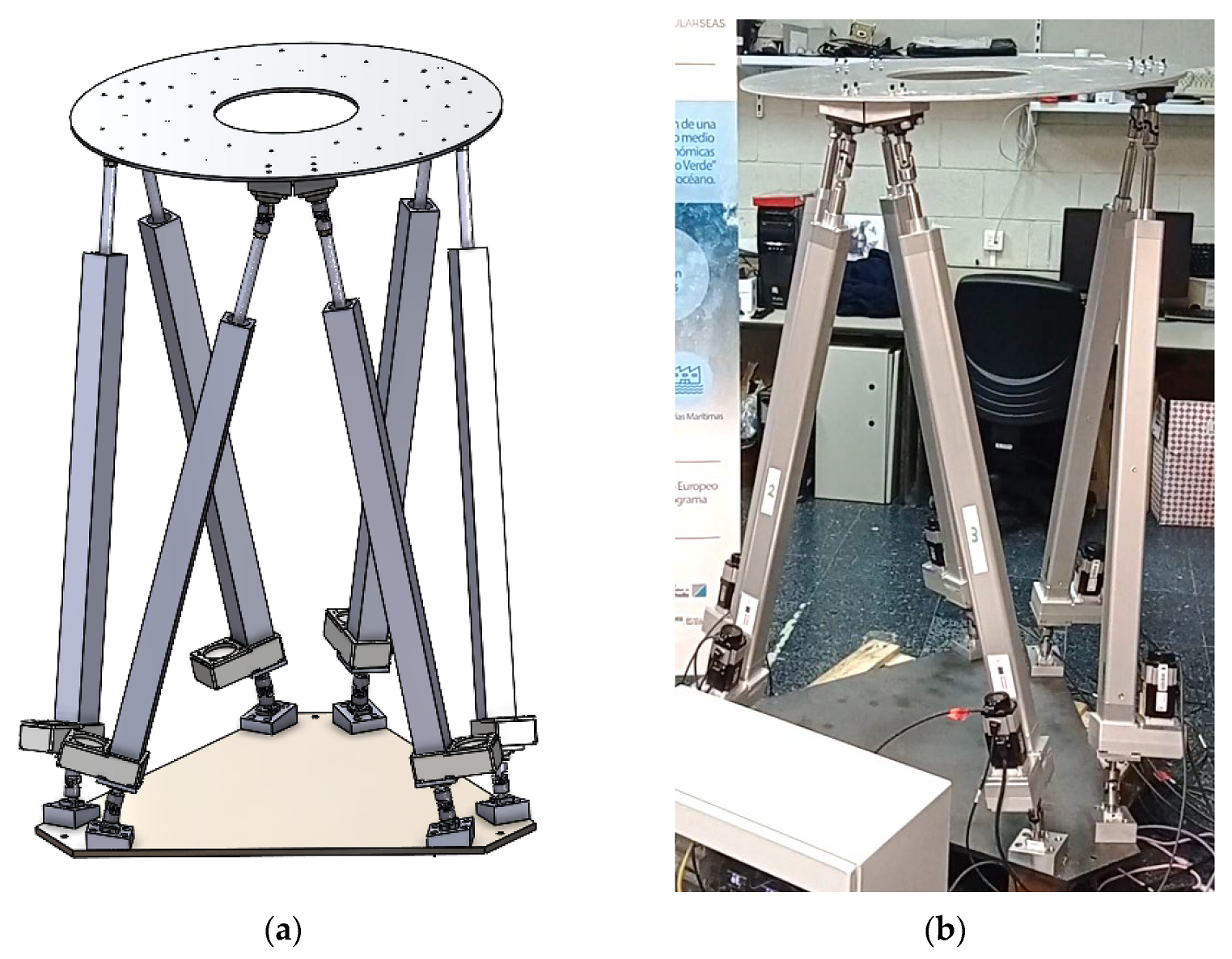
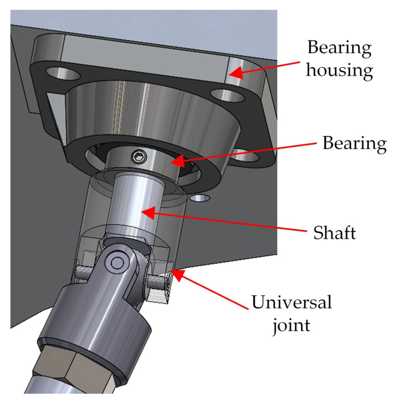
2.3. Particularities of the Mechanical Design

The following particular mechanical design decisions were made with regard to the Stewart Platform in this study in order to comply with the 6-DOF. The use of a Stewart Platform to emulate wave movements was framed within the CircularSeas project as a way to systematically examine how oceanic conditions affect on-board 3D printing. Some design requirements, which are related to the parameters in Table 1, were the following: platform diameter not greater than 1.10 m to operate in narrow environments, resulting in the base radius, r b ; dimensions of the 3D printers to be moved by the platform, with a volume ranging from 342 mm × 460 mm × 580 mm to 490 mm × 503 mm × 1357 mm, thus resulting in the upper platform radius, r p ; load (3D printers) weight of up to 50 Kg. In order to simulate oceanic movements, maximum speeds and accelerations of at least 0.6 m/s and 6 m/s2, respectively, and up and down movements of approximately 600 mm were required. These requirements drove the selection of the cylinders and the parameter, l 0 . The values of the variables h b and h p as well as the height of the platform in its initial position, h 0 , were dependent on the designed structural parts and the selected universal joints. Finally, the assembly angles between the hinges of the base and the mobile platform ( φ b and φ p ) were extracted from the CAD design. All measurements were verified on the CAD design and on the real platform used in this research (Figure 1b).
A combination of bearing with housing, shaft, and universal joint assembly was used to make the connection between the upper platform and the cylinders, as can be seen in Figure 3. The combination of bearing and universal joint allowed each cylinder to rotate about its axis, with each joint therefore acting as a spherical joint [65,78]. This design decision was taken to avoid expensive spherical joints.
Following some studies in the literature [75,79], two specific mechanical components made of aluminum were designed to obtain a resting position with no angle in the universal joints, as is highlighted with a red circle in Figure 4.
Each electromechanics cylinder was mounted with a parallel coupling system with the servomotor. A connecting part was designed to specifically connect the coupling system with the universal joints (parts 2 and 3 of Figure 5). These parts also fit the shaft attached to the universal joint. In addition, each universal joint had a set screw to assist in centering and securing the shaft.

3. Platform Kinematics

3.1. Inverse Kinematics

The closed-loop vector approach was considered to conduct the analysis of the direct and inverse kinematics (Figure 6).
Two Cartesian axes were placed at the center of the base platform B x y z   and the moving platform P x y z , as can be seen in Figure 6. The origin of the base coordinate system was at the point [0,0,0] represented by B . The points B i and P i in Figure 6 represent the connection points of each member (denoted by L i ) to the base and mobile platforms, respectively. In Figure 6, the notations of B i = B i x ,   B i y ,   B i z and P i =   P i x ,   P i y ,   P i z represent the vectors connecting the above connection points to the origin of each coordinate system, counter-clockwise about the positive Z-axis. The vector X d = x ,   y ,   z relates the desired position of the coordinate system P to the coordinate system B . Thus, the vector relationship for each member, L i = L i x ,   L i y ,   L i z , is given by Equation (8):
L B i = P B i + X B d     B B i
The value of the vector P B i , which connects the mobile platform member’s junction points with the B coordinate system, can be found using Equation (8). In this equation, it is necessary to apply a Roll-Pitch-Yaw rotation matrix ( R P B ) to the vector P P i . The rotation matrix has the rotation angles γ on the X-axis, β on the Y-axis, and α on the Z-axis, as given in Equation (8), where “c” stands for cosine and “s” for sine.
R z α = c α s α 0 s α c α 0 0 0 1 , R y β = c β 0 s β 0 1 0 s β 0 c β , R x γ = 1 0 0 0 c γ s γ 0 s γ c γ
R P B = R z α   R y β   R x γ = c α   c β c α   s β   s γ s α   c γ c α   s β   c γ + s α   s γ s α   c β s α   s β   s γ + c α   c γ s α   s β   c γ c α   s γ s β c β   s γ c β   c γ = r 11 r 12 r 13 r 21 r 22 r 23 r 31 r 32 r 33
P B i = R P B P P i = r 11 r 12 r 13 r 21 r 22 r 23 r 31 r 32 r 33 P i x P i y P i z = r 11 P i x + r 12 P i y + r 13 P i z r 21 P i x + r 22 P i y + r 23 P i z r 31 P i x + r 32 P i y + r 33 P i z = u i v i w i , i = 1 . . , 6
The subtraction of the end-effector positioning vector and the vector of the base member platform attachments can be grouped into the displaced auxiliary vector d B i , according to Equation (9):
d B i = X B d B B i = x B i x y B i y z + h 0 B i z = x i ¯ y ¯ i z i ¯
It can also be noted that h 0 is the separation distance between platforms from center to center in the resting position. Equation (11) is then obtained by considering Equations (5) and (9):
L B i = P B i + d B i
Therefore, the value of the elongation of the prismatic joint, l i , with the use of geometric inverse kinematics, is the norm of the L B i vector (Equation (11)):
l i = L B i = L i x 2 + L i y 2 + L i z 2 = x i ¯ + u i 2 + y i ¯ + v i 2 + z i ¯ + w i 2 , i = 1 . . , 6
As the actuators were electric cylinders, l i does not consider the length of the cylinders when they are fully retracted ( l 0 ) [33,58,80]. Therefore, the real position in the joint space needs to consider the length of the retracted drive rod.
q i = l i l 0 , i = 1 . . , 6

3.2. Direct Kinematics

Direct kinematics is based on obtaining the position and orientation of the end-effector from the length values of each linear actuator. This involves finding a closed-form solution containing six simultaneous non-linear equations with six unknown variables and different possible solutions. As mentioned above, the Newton–Raphson iterative numerical method was employed to solve this problem.
The first step lies in the definition of the i t h scalar functions that show the difference between the calculated length of the actuators and the actual measured length, as shown in Equations (13) and (14).
f i a = x i ¯ + u i 2 + y i ¯ + v i 2 + z i ¯ + w i 2 L i 2 = 0
f i a = L a 2 L i 2 = 0
This function is applied on the a vector (Equation (15)), which groups the position and orientation to be obtained.
a = a 1   a 2   a 3   a 4   a 5   a 6 T = x   y   z   α   β   γ T
The Newton–Raphson method applied to this case returns the following expression (Equation (16)):
a n + 1 = a n F a n a 1 F a n
where a n represents the current position value, a n + 1 denotes the new position iteration value, and F a n is the matrix of differences between the calculated and measured values in the displacement length of each actuator for each element of the current position’s iteration value. The matrix F a n a 1 is mathematically equivalent to the inverse Jacobian of F a n at each current iteration value, and Equation (16) can be rewritten into Equations (17) and (18):
a n + 1 = a n J 1 a n   F a n
x y z α β γ n + 1 = x y z α β γ n f 1 x f 1 γ f 6 x f 6 γ n 1 f 1 f 2 f 3 f 4 f 5 f 6 n
Solving the above system of matrix equations gives the value of the newly calculated position. Finally, the values of the newly calculated position and the current one are subtracted. If the difference between the two values in all dimensions of the vector is less than the limit of convergence, the solution is considered valid, and we have the solution of the direct kinematics. If not, the newly calculated point is taken as the current point, and a new point is recalculated until convergence is obtained.
Both inverse and direct kinematics are used when carrying out the movement of the platform. The first one is employed to realize the movement by converting the Cartesian point into the movement of the cylinders. The second is used, among other applications, to obtain the starting point of the movement. The generation of trajectories is described below.

3.3. Trajectory Generation

This section addresses the trajectory generation that was implemented on the Stewart Platform to carry out PTP and oceanic wave motions.

3.3.1. Point-to-Point Trajectory

A point-to-point (PTP) path planning algorithm based on cycloidal trajectories was implemented to move the robot along a straight path in any of the six spatial coordinates. These trajectories had zero velocity and zero acceleration at the beginning and end of the movement. In the literature, we can find these cycloidal algorithms being applied on Stewart Platforms and manipulators although under the name of Kane’s transition function [32,81,82,83,84,85]. However, when Kane tackled the problem of trajectory generation for PTP sections, he decided to arbitrarily use this type of trajectory [86], which is nothing more than a cycloidal function. When considering the cycloidal trajectory equations of position, speed, and acceleration in Equations (19)–(21), respectively, six constraints in displacement, speed, and acceleration can be found, both at the start and at the end, as shown in Equation (22).
p t = p T p 0 t T 1 2 π sin 2 π t T + p 0
p ˙ t = p T p 0 T 1 cos 2 π t T
p ¨ t = 2 π p T p 0 T 2 sin 2 π t T
p 0 = p 0 , p T = p f , p ˙ 0 = 0 , p ˙ T = 0 , p ¨ 0 = 0 , p ¨ T = 0
where T is the difference between the final time and the initial time, p t is the current position at a given current time t , p 0 is the initial position, p f is the final position to reach, t 0 is the initial time, and t f is the final time of the movement.
Among the advantages of using this algorithm instead of others—such as cubic polynomials, quintic polynomials, etc.—two stand out. First, it is an algorithm based on trigonometric functions that present non-null continuous derivatives for any order of derivation in the interval ( t 0 , t f ) [87]. Consequently, the specific cycloidal trajectory presents a continuous acceleration profile (acceleration is finite at all times), thus obtaining a movement with lower characteristics of vibration, tension, noise, and shock [88]. This makes it a suitable trajectory for high-speed applications where low residual vibration (vibration after the end of the motion segment) is desired. Indeed, in [89], they suppressed residual vibration in PTP motion by using cycloidal functions. It has also been widely used for steady and continuous motion [90], which is very important for motors to be able to start and stop more softly. Second, it incorporates the trigonometric functions into the motion laws to enhance the ease of their implementation [91]. When generating points that can move the joints synchronously on the Stewart Platform, a kinematic scaling of the trajectory can be performed by means of a normalized parameter. This ensures compliance with the maximum acceleration and maximum velocity constraints. Therefore, given a trajectory p t , the normalized form is obtained using Equation (23):
p t = p i + h   σ τ
where p i is the initial point, h is the difference between the initial and final positions, and σ τ is the value determined by Equation (24):
σ τ = τ 1 2 π sin 2 π τ , 0 σ τ 1
which τ is the time taken to navigate the segment, and is represented by Equation (25):
τ = t t 0 T , 0 τ 1
Therefore, the normalized position equation can be derived to obtain velocity, acceleration, and jerk with Equations (26)–(28), respectively. The maximum values to consider in the kinematic constraints of the trajectory are obtained by applying the chain rule to the change in the temporary variable described above. The kinematic constraints can be satisfied by modifying the duration of the trajectory, T .
σ ˙ τ = 1 cos 2 π τ , p ˙ m a x = 2 h T
σ ¨ τ = 2 π sin 2 π τ , p ¨ m a x = 2 π h T 2
σ τ = 4 π 2 cos 2 π τ , p m a x = 4 π 2 h T 3
An example of Cartesian motion for a span of 30 mm in 3 s and a velocity of up to 20 mm/s is shown in Figure 7:

3.3.2. Oceanic Wave Motion

Deep-sea ocean wave-type motion on the surface was implemented as the basis for the oceanic wave motion, which was performed by the developed Stewart Platform. A given linear wave in the domain of space can be represented by a sinusoidal profile using Airy’s wave theory [92]. A wave is characterized by the following set of parameters: the wave number ( k ), the number of times a wave vibrates at a given distance; the wavelength ( L ), the distance between the same points between two consecutive oscillations; the period ( T ), the time it takes for a wave to complete a full oscillation; the angular frequency ( w ), the frequency of the wave in radians per second; and the amplitude ( A ), the distance between the point of maximum elongation of a wave and its midpoint and frequency.
The function that governs the movement of the free surface of the sea ( η ) considering the distance measured x ˜ along the horizontal axis is expressed by Equation (29):
η x ˜ ,   t = A   cos k x ˜ w t
where k is 2 π / L and w is 2 π / T .
The classical nomenclature in wave theory does not assume the effect of all the frequencies that appear in reality. A real wave, also called a random wave, is a wave that can be decomposed into a finite number of linear waves with the frequencies that comprise it and different amplitudes [93]. Therefore, it can be seen as the sum of a large number of linear harmonic wave components in a Fourier analysis.
η x ˜ , t = i = 1 N A i   cos k i x ˜ w i t + ϕ i
where η x ˜ , t is the variation of the sea surface at a given time and at a given point of the displacement direction of the wave, N is the total number of linear waves in the decomposition, A i is the amplitude of the i t h linear wave, w i is the angular frequency of the i t h wave, and ϕ i is the phase of the i t h wave. Figure 8 shows an example of the random wave decomposition.
Summing up, the generation of the motion of an ocean wave in this study was treated as a sine wave with Airy’s linear theory and as the composition of sinusoids (random wave).
Up to this point, the variation profile of the free sea surface with a mean water level of zero η is obtained, which is directly on the Z-coordinate on the surface. However, a particle of a travelling ocean wave in the deep sea moves along circular orbits [94]. This particle has a horizontal ξ and a vertical ς displacement, which are shown in Equation (31). The detailed development of particle trajectories in the deep sea can be found in [95].
ξ = A   e k   η sin k x ˜ w t ς = A   e k   η cos k x ˜ w t
In addition, it is possible to consider the surface displacement of a wave travelling at an angle to the axis of displacement to have the horizontal motion of the particle at 2 DOF [96]. To do so, the particle path is multiplied by a “wave attack” angle θ . This approach was the one taken by Galván-Pozos and Ocampo-Torres in their research [57]. The oceanic wave motion expressed in Cartesian coordinates to generate the motion of the Stewart Platform is shown in Equation (32):
x = A e k   η sin k x ˜ w t cos θ y = A e k   η sin k x ˜ w t sin θ z = A   e k   η cos k x ˜ w t
Equation (33) shows the angular displacement of the oceanic wave motion. This is given by the slope of the tangent to the free surface at each point in the X and Y directions. In the Z-direction, it is considered as zero since horizontal angular movements are still a relatively small value [54].
α = tan 1 d η d x β = tan 1 d η d y γ = 0
The groundwork for the modelling, kinematics, and motion generation of the Stewart Platform developed in this study has been presented. The next section will focus on detailing its implementation through an automation architecture based on the use of industrial controllers.

4. Control Automation with Industrial Resources

4.1. Architecture

The Stewart Platform developed for this study is automated by an industrial controller. These are seen as PLCs with numerical control capabilities for motion control tasks. In general, axis controllers are programmed according to the PLCopen Motion Control automation standards, which define a reusable set of function blocks (FB) for the implementation of the industrial servomotor’s motion. The industrial controller employed in this research is an OMRON NJ501-1300.
Six electromechanical cylinders were chosen for the linear displacement of the “legs” of the platform. These electromechanical cylinders are driven by industrial servomotors that have built-in absolute encoders to obtain position–velocity feedback. With this feedback, it is possible to estimate the overall platform position by using the direct kinematics, as mentioned in Section 3.2.
Figure 9 presents the architecture for implementing the motion of any parallel robot with an industrial controller, such as the Stewart Platform in this study. The architecture is divided into five main tasks: a plc task, a motion control task, a communications task, a servodrive task, and a real motion task. The PLC task is the one that the user defines, while the other tasks are typically hidden from the user’s view and can only be parameterized, without the possibility of altering their order of execution.
The industrial controller runs any program containing a general process, which can involve some machines. When the motion of the platform is requested in the program, the PLC task is the one responsible for the sequence control management. Based on a desired motion of the platform—for example, a PTP straight line through the X-axis—the industrial controller plans the sequence and gives the data to the toolpath generator. The toolpath generator addresses the calculus of the actual position of the platform (direct kinematics), the generation of motion profiles in the cartesian toolpath according to the type of motion, and the inverse kinematics in order to transform it into a set of toolpaths for the six joints. For each cycle, a new set of six setpoints are sent to the motion sequence part of the task. The particularities of the implementation of motion generation in the industrial controller will be detailed in the subsequent sections.
The next step involves the specification of the current commanded setpoint to the servomotors through the motion sequence, which is the type of sequence that is responsible for generating motion in any motor configured in the program using the MC Function Blocks defined by PLCopen. There are a few manufacturers that implement a user-defined cycle-by-cycle generation of the trajectory, which could be affected by changes in trajectory during its execution. In a Stewart Platform robot, all the joints should move synchronously, and therefore the motion control resources need to ensure the cyclical motion. To do so, the MC_SyncMoveAbsolute Function Block was employed. The use of this type of block not only affects the commanded position, but also the PLCopen data structure of each axis of movement, thus altering its internal state and other variables. Therefore, at this point, six axis-commanded point-to-point positions with the full data structure of each axis are sent to the motion control task, also called the MC primary period task.
Currently, axis controllers use specific internal tasks to carry out motion control functions. The controller needs the information from the user program, which is exchanged by using any motion control function block. Internally, the controller gathers the information of the commanded motion and performs an interpolation that considers the real position taken from the encoder feedback (profile and synchronization processing), as shown in Figure 9. The commanded position in the previously configured units, e.g., millimeters, is obtained from the interpolation. However, the servodrive needs pulses. Therefore, the final step of the motion control task addresses the relationship between the display unit (the work travel distance per motor rotation) and the pulse unit (the command pulse count per motor), also called the internal electronic gear.
The pulses are sent by the EtherCAT master function task. EtherCAT is a fast, standard, master–slave-based industrial Ethernet technology that can support a synchronized cycle time of up to 100 μs. In addition, sensor and actuator devices, such as industrial servomotors, from different suppliers can be integrated without any problems, provided they have EtherCAT interfaces. Therefore, to establish an open-structured and reconfigurable hardware platform, the EtherCAT bus is adopted. This EtherCAT Function Module exchanges data with the servodrive using the CoE (CAN application protocol over EtherCAT). CoE technology can specify parameters and motion control data mapping using the object dictionary of each servodrive. Process data objects (PDOs) and service data objects (SDOs) communicate the data between the industrial controller and the servodrive. PDOs periodically exchange data in real time, such as the servomotor position control, and SDOs exchange data when required, such as for parameter transfers.
Each servodrive has an internal task that converts the pulses to electric PWM signals. After the communication processing and command interpretation, the setpoint commands are introduced through a cascade loop of PIDs in order to achieve the proper position, velocity, and torque considering the limits of the motor. To do so, the servodrive implements a tracking error strategy that considers the setpoint and handles the current position from the axis encoder.
Finally, the “real task” addresses the motion of a load on the platform composed of six electromechanical cylinders (UNIMOTION PNCE-50-BS-2010-600-S was used in this study) driven by industrial servomotors with absolute encoders (R88M-1M40030H/T was used in this study). Among the different types of coupling that can be made between a cylinder and the engine, the parallel-type coupling was chosen to avoid increasing the height of the platform.

4.2. Motion Implementation

As mentioned above, to perform the motion of the Stewart Platform, some kinematic calculations and trajectory generation are needed. This section details the algorithms and particularities of the implementation in an industrial controller. All algorithms as well as the process sequence and motion generation, among others, were implemented in the NJ501-1300 controller following the Structured Text programming language, which is a standard IEC 61131-3 programming language for industrial controllers.
A point-to-point movement requires a target point and the speed at which the platform will move to reach that point. Thus, the initial and final times of the movement are obtained for each of the spatial variables. The current point is then calculated with direct kinematics to obtain the starting point of the trajectory generator. The trajectory generator, which considers the speed, acceleration, and jerk limits, calculates the spatial points through which the Stewart Platform will move at each automaton cycle until it reaches the target position. Each spatial point is passed through the inverse kinematics to obtain the target displacement of the cylinder that reaches the spatial position. Finally, each cylinder displacement is executed in the axis controller by the function block “MC_SyncMoveAbsolute”, from the user program in every task period to the servodrive.
Therefore, Algorithm 1 was employed to obtain the inverse kinematic solution (implementation of Equations (5)–(12)).
Algorithm 1: Inverse Kinematics
Input: Spatial point to reach, ( P B i n p u t ); fully retracted length of cylinders, ( l 0 )
Output: An array with the length of each cylinder in the joint space ( q a c t )
 
Matrix rotation, ( R x y z );
1  R x y z ← Computation of the rotation matrix considering the P B i n p u t spatial orientation
2 foreach cylinder
3   P B i ← Perform the coordinate system transformation of P P i
4   d B i ← Computation of the difference between P B i n p u t and B B i
5   L B i ← Calculus of the total length vector for each cylinder
6   q a c t   i ← Adaptation of the length vector norm considering the real cylinder
     ( L B i   l 0 )
7 end foreach
However, several factors had to be taken into account in the direct kinematics. Industrial controllers have a cycle time within which to perform all the instructions of a program. Furthermore, such devices do not have the computing power to perform function derivatives, recursive calculations, or complex matrix equations on their own. Therefore, in order to implement the inverse Jacobian from the Newton–Raphson method in industrial controllers, an exhaustive simplification of each element of the Jacobian matrix was chosen. This simplification approach can also be found in the literature, e.g., in [97], where the main differences are (1) in the computation of the partial derivatives, which is the appearance of the terms associated with the z-coordinate of the P P i vector, since this value in this study is non-zero due to the phase shift introduced by the height of the universal joints mentioned in Section 2; (2) in the positive sign of x i ¯ in f i β . Considering Equation (9), the result of the partial derivatives of x, y, and z is obtained (Equation (34)). Moreover, the result of the partial derivatives of u i , v i , and w i with respect to the α , β , and γ angles can be obtained using Equations (7) and (8), just as Equation (35) is after comprehensive simplification. Hence, the cycle time is shortened by exploiting some of the calculations previously made, such as the elements that make up the rotation matrix (r11 to r33).
x i ¯ x = y i ¯ y = z i ¯ z = 1
u i α = v i ,     u i β = c α   w i ,     u i γ = P i y r 13 P i z r 12 v i α = u i ,     v i β = s α   w i ,     v i γ = P i y r 23 P i z r 22 w i α = 0 ,     w i β = c β   P i x s β s γ   P i y s β c γ P i z ,     w i γ = P i y r 33 P i z r 32
Given Equations (34) and (35), the value of each element of the Jacobian can be calculated (Equation (36)). This equation represents the set of values to efficiently implement in the industrial controller.
f i x = 2 x i ¯ + u i f i y = 2 y i ¯ + v i f i z = 2 z i ¯ + w i f i α = 2 y i ¯ u i x i ¯ v i f i β = 2 x i ¯ c α + y ¯ i s α w i c β P i x + s β s γ P i y + s β c γ P i z z i ¯ f i γ = 2 x i ¯ r 13 + y i ¯ r 23 + z i ¯ r 33 P i y x i ¯ r 21 + y i ¯ r 22 + z i ¯ r 32 P i z
Regarding the implementation of the inverse of the Jacobian in an industrial controller without the use of an external software (e.g., MATLAB, Simulink, Labview), one of the properties of invertible square matrices is used. This property states that the multiplication of a matrix by its inverse results in an identity matrix of the same order as the first matrix, provided that the determinant of the matrix is non-zero (greater than a tolerance limit near to zero). However, the resolution of the determinant has to be possible since PLC and industrial controllers’ programming languages do not usually support linear algebra tools such as matrix operations (and when they do implement them, they are the most basic for small matrices). Therefore, for the computation of the determinant of a 6 × 6 matrix in an industrial controller, it is necessary to implement an ad hoc solution in the controller. Since there is no possibility of applying recursive methods in the PLC [98], such as the cofactor expansion method, the Leibniz formula was implemented as it is widely used for calculating matrix determinants [99]. Once the determinant was calculated, the result was checked to ensure that it was less than a threshold—which is a value close to zero—in order to avoid computational inaccuracies. An example of a threshold value used to detect singular values in the vicinity of zero in the determinant of the Jacobian matrix can be found in [100]. After ensuring that F is a non-singular matrix (determinant distinct to zero), the inverse of the Jacobian matrix is calculated, considering that it is an unknown parameter in a linear algebraic matrix equation. Therefore, the LU decomposition method, which is often used as one of many possible expedient algorithms to find the inverse of a matrix [101], was used. The LU decomposition method was implemented following Doolittle’s algorithm, a compact algorithm that achieves a low computational cost [102].
Finally, to avoid the industrial controller watchdog constraints due to the while loop in the direct kinematics algorithm, an iteration count was employed, which allowed for the controller to finish its current cycle and follow the calculation of the direct kinematics in the following cycle when needed.
Summing up, Algorithm 2 was employed in the industrial controller to obtain the direct kinematic solution.
Algorithm 2: Direct Kinematics
Input: An array with the actual length of each cylinder ( L a c t ); first iteration point, ( P f i r s t );
Output: Actual spatial point of the end effector ( P s o l )
 
Convergence limit, ( K l i m );
Tolerance, ( K t o l );
Current iteration point, ( P c u r r e n t );
Difference between current iteration point and calculated point, ( D p );
Point calculated from Newton–Raphson equation, ( P c a l c );
Matrix of scalar function F in Equation (14), ( F n );
Jacobian of the F n matrix, ( J n );
Jacobian inverse ( J n 1 );
1 P c u r r e n t ← Assign the first iteration point P f i r s t to the current iteration point
2do
3   L c a l c  ← Computation of inverse kinematic over the first iteration point
4   F n  ← Calculus of the matrix F
5   J n  ← Computation of the Jacobian matrix
6  det( J n ) ← Calculus of the Jacobian determinant
7  if (abs(det( J n )) > K t o l ) then
8    J n 1  ← Compute the inverse of J n using LU decomposition
9    P c a l c  ← Solve the Newton–Raphson equation to obtain the calculated point
10    D p  ← Absolute difference of P c a l c and P c u r r e n t for each coordinate
11    P c u r r e n t ← Update current point based on the calculated point, P c a l c
12  else
13   Exit due to singularities in the Jacobian matrix
14 while (Dp > Klim)
15  P s o l ← The solution is the last current point of the Newton–Raphson method
Regarding the ocean wave motion generator, the strategy is almost the same as in the PTP. If the motion to perform is based on the simple Airy theory, the wavelength, amplitude, frequency, and phase of the wave are needed, as well as the angle attack to the x-y motion. The first step is to obtain the first point using direct kinematics. Then, without carrying out any movement, the generation of ocean trajectories for the first point is executed to obtain the initial point of the wave motion. A point-to-point movement for this initial wave point is then carried out. This is performed in order to avoid a large gap between the current point of the platform and the initial point of the wave, since by having cosine-dependent variables when starting the movement with a zero angle, the maximum amplitude is obtained in one of the coordinates. This prevents a single task cycle from being given an unreachable setpoint that would cause the platform to enter into error. Once at the initial point of the wave, the generation of the ocean movement while considering all the input parameters is started. The inverse kinematics is executed at each point of the oceanic trajectory to convert it to the effective movement of the cylinders. Finally, each cylinder displacement is executed using the “MC_SyncMoveAbsolute” motion control function, as in the previous case.

5. Results

This section presents the results obtained by implementing inverse kinematics, platform motion, and direct kinematics in the NJ501-1300 industrial controller in order to evaluate the performance of automation based on the use of an industrial controller architecture and industrial resources.

5.1. Inverse Kinematics Implementation: Cycloidal and Oceanic Wave Trajectories

Several trajectory movements were performed using the trajectory generation algorithm and the inverse kinematics mentioned in Section 3. Once the speed and end points were selected in the user program, the trajectory was automatically generated and the movement started. Some examples are given below to show the movement of the trajectory tracking.
Figure 10 shows a series of PTP movements performed from the starting point p i n i = 0   mm ,   0   mm ,   150   mm ,   0 ° ,   0 ° ,   0 ° T and how the cylinders move with respect to these defined trajectories after applying the inverse kinematic solution. These movements were performed in each of the mechanism’s degrees of freedom. The trajectories performed in the X, Y, Z coordinates were made from 100 mm absolute at 20 mm/s, as can be seen in the first three plots in the column on the left of Figure 10. The trajectories performed in the α ,   β ,   γ coordinates were 6°, 6°, and 10°, respectively, at a speed of 2°/s, as can be seen in the last three graphs in the column on the left-hand side. The column on the right-hand side shows the different positions that the cylinders reached to follow the trajectory described in their respective movements in the column on the left-hand side.
The next test involved the ocean movement based on the trajectory generation reviewed in Section 3.3.2 for the simple Airy wave and the random wave. Figure 11a shows how the Cartesian spatial point varies for a wave with an amplitude of 3 mm, a 10° phase, a period of 10 s, and a wavelength of 100 m; Figure 11b shows the response of the cylinders to this type of motion.
Figure 12 presents the time evolution of the spatial trajectory of the Stewart Platform under a wave following the random wave model. This random wave was composed of five sinusoidal waves with the parameters below (Equation (37)). The response to the movement of the cylinders can be seen in Figure 12b. Both Figure 11 and Figure 12 started with the positioning phase at the starting point of the oceanic movement. When this point was reached, the ocean wave motion began.
A = 3 ,   2.3 , 3.5 ,   0.7 ,   5.4   mm T = 10 ,   5 ,   3 ,   7 ,   3   s L = 60 ,   85 ,   75 ,   70 ,   100   mm ϕ = 10 ,   15 ,   0 ,   20 , 45   °

5.2. Performance of Direct Kinematics

To evaluate the performance of the implementation of the direct kinematic in industrial controllers, the following test was executed.
This test was based on moving the platform to certain points within its workspace and—from an initial point of iteration of the direct kinematics and an established convergence—on solving the direct kinematics, quantifying the point obtained, and estimating the time it took to reach the result. Both the initial iteration point and the convergence limit were the same for all the tests in order to measure how it affected the fact that the platform was already positioned more or less close to the initial iteration point. All tests were performed with a 1 ms automaton cycle. The following table shows the results obtained after eight position calculation tests with direct kinematics. The convergence of the Newton–Raphson algorithm was fixed at 0.01, and the initial iteration point was p N R = 60.25   mm ,   85   mm ,   230.7   mm ,   0 ° ,   0 ° ,   3.75 ° T . The selected starting point was a fixed parameter in order to be able to study the performance of direct kinematic implementation when this point is further away from or closer to the real position of the robot. Nevertheless, there are already reported specific methods with which to choose the starting point when applying the Newton–Raphson method, which can improve the computational speed and convergence [103].
It can be seen that in the farthest case tested, the algorithm required 13 iterations to reach the correct solution with high accuracy, which is approximately 640 μ s, more than half of the most demanding duty cycle of the industrial controller tested.
These results show that it is possible to implement the calculation of direct kinematics with industrial controllers in real time and with high accuracy as the target points are always reached within the convergence limit, without heavily compromising cycle time.
Finally, the calibration procedure for the platform is performed, first by moving all equal cylinders up to their retracted (rest) position. Once in this position, the initial height of the platform and the initial length of the cylinders that are shown in Table 1 are checked, as well as the levelness of the upper platform. After this calibration, a rotation data counter setting is established on the absolute encoders of the servomotors in order to set them as the zero of the cylinders. This measurement is then transferred to the servodrives so as to be stored in their internal memory. At this point, the platform is at the origin (coordinates [0,0,0,0,0,0]). Then, discrete and individual movements are made to check the longitudinal displacements and rotations by positioning digital measuring devices at predefined points of the platform.

6. Discussion

This study set out with the aim of assessing the control automation strategy for performing point-to-point and oceanic wave motions with industrial resources. The point-to-point motion obtained as the kinematic solution in Figure 10 is in accordance with the motion of other Stewart Platforms found in Simulink simulations with electric cylinders in the literature [77,82].
Furthermore, the solution for the inverse kinematics of the oceanic motion of particles on the surface of a deep-sea-type ocean behaves rather similar to those found in studies that modelled the motion of deep-sea particles. [57,104]. The generation of the ocean wave motion went into the detail of the ocean wave model, and it differs from other works by researchers that produced movement similar to that of the ocean through the generation of Cartesian points with sinusoidal functions, which had been obtained experimentally within a simulation environment [34,54,58].
As some studies addressed [105,106], when implementing direct kinematics in real time in order to track trajectories, specifying points that are close to each other makes the algorithm converge much faster. However, in order to be useful in real-time trajectory control, if any movement is performed every millisecond, the solution of the direct kinematics has to be less than one millisecond, taking into account the fixed execution time and the user-defined program time. In some cases, in order to comply with the fastest industrial controller task cycle, there may be a need to divide these calculations into more than one task cycle. Therefore, high-level functions in trajectory-following control must consider this delay. Some research works reported that the kinematic solution is complex and resource-heavy to calculate in real time [34,107]. However, the results in Table 2 support the idea that the implementation can be executed efficiently in real time with an accurate position solution. Considering that the typical cycle time of an industrial controller is between 1 ms and 10 ms, obtaining accurate results in less than 1 ms validates the real-time efficiency.
The advantage of being able to include direct kinematics at runtime is that it would allow for a fast control cycle to be performed during automation, and at a high level for those control loops that would already be taking place in the servodrive. In this way, automation decisions can make it more complex for position control to close the loop in the industrial controller, or for high trajectory speed monitoring tasks such as error tracking, margin checking, etc.

7. Conclusions

The purpose of the current study was to investigate the control automation of a Stewart Platform using only the resources provided in today’s industrial controllers. To support this, modelling, inverse and direct kinematics as well as cycloidal PTP and oceanic wave motion were implemented in an industrial controller. One of the more significant results is that it is possible to perform the direct kinematic calculations with high accuracy in real time by employing industrial controllers.
This brings about some practical applications. Firstly, it points to the architecture and strategy needed to automate any parallel robot in order to perform spatial motion with current industrial controllers without using third-party software. Secondly, two different types of positioning strategies for Stewart Platforms are detailed along with their benefits: cycloidal point-to-point and oceanic wave motions based on the single Airy wave model and irregular waves. Thirdly, it shows an effective way to calculate the direct kinematics on the controller side, which may open the possibility of closing the positioning loop on the controller or implementing supervisors such as the “tracking error”.
Further research might investigate the effects of planning the sequence of the trajectory in order to avoid commanding points outside the workspace and collision with objects inside the workspace while considering the feedback of the tracking error. Moreover, having such a robot automated with an industrial controller allows for easy and direct integration with other more complex industrial servo axis systems.

Author Contributions

Conceptualization, J.G.; methodology, J.G. and D.S.; software, J.G. and D.S.; validation, J.G.; formal analysis, J.G. and D.S.; investigation, J.G. and D.S.; resources, E.R.; data curation, J.G. and E.R.; writing—original draft preparation, J.G. and D.S.; writing—review and editing, J.G. and D.S.; visualization, J.G. and E.R.; project administration, J.G.; funding acquisition, J.G. All authors have read and agreed to the published version of the manuscript.

Funding

This work was supported by the European Regional Development Fund (ERDF): Interreg Atlantic Area Programme, grant number EAPA_117/2018, within the framework of the CircularSeas Project. The APC was funded by the ERDF: Interreg Atlantic Area Programme.

Institutional Review Board Statement

Not applicable.

Informed Consent Statement

Not applicable.

Conflicts of Interest

The authors declare no conflict of interest.

References

  1. Jin, Y.; Chanal, H.; Paccot, F. Parallel Robot. In Handbook of Manufacturing Engineering and Technology; Nee, A., Ed.; Springer: London, UK, 2014; pp. 1–33. ISBN 978-1-4471-4976-7. [Google Scholar]
  2. Shao, Z.-F.; Tang, X.; Wang, L. Dynamics Verification Experiment of the Stewart Parallel Manipulator. Int. J. Adv. Robot. Syst. 2015, 12, 144. [Google Scholar] [CrossRef]
  3. Alvarado Requena, E.; Estrada, A.; Ramírez, G.T.; Elias, N.R.; Uribe, J.; Rodríguez, B. Control of a Stewart-Gough Platform for Earthquake Ground Motion Simulation. In Industrial and Robotic Systems; Hernandez, E.E., Keshtkar, S., Valdez, S.I., Eds.; Mechanisms and Machine Science; Springer International Publishing: Cham, Switzerland, 2020; Volume 86, pp. 138–146. ISBN 978-3-030-45401-2. [Google Scholar]
  4. Stewart, D. A Platform with Six Degrees of Freedom. Proc. Inst. Mech. Eng. 1965, 180, 371–386. [Google Scholar] [CrossRef]
  5. Hunt, K.H. Kinematic Geometry of Mechanisms; Oxford Engineering Science Series; Clarendon Press: Oxford, UK; Oxford University Press: New York, NY, USA, 1978; ISBN 978-0-19-856124-8. [Google Scholar]
  6. Dasgupta, B.; Mruthyunjaya, T.S. The Stewart Platform Manipulator: A Review. Mech. Mach. Theory 2000, 35, 15–40. [Google Scholar] [CrossRef]
  7. Porta, J.M.; Thomas, F. Yet Another Approach to the Gough-Stewart Platform Forward Kinematics. In Proceedings of the 2018 IEEE International Conference on Robotics and Automation (ICRA), Brisbane, QLD, Australia, 21–25 May 2018; IEEE: Brisbane, QLD, Australia, 2018; pp. 974–980. [Google Scholar]
  8. Staicu, S. Dynamic Analysis of the 3-3 Stewart Platform. UPB Sci. Bull. D 2009, 71, 3–18. [Google Scholar]
  9. Shao, Z.-F.; Tang, X.; Wang, L.-P. Optimum Design of 3-3 Stewart Platform Considering Inertia Property. Adv. Mech. Eng. 2013, 5, 249121. [Google Scholar] [CrossRef] [PubMed]
  10. Rastegarpanah, A.; Saadat, M.; Rakhodaei, H. Analysis and Simulation of Various Stewart Platform Configurations for Lower Limb Rehabilitation. In Proceedings of the 4th Annual BEAR PGR Conference 2013, Birmingham, UK, 16 December 2013. [Google Scholar]
  11. Alp, H.; Anli, E.; Özkol, İ. Neural Network Algorithm for Workspace Analysis of a Parallel Mechanism. Aircr. Eng. Aerosp. Technol. 2007, 79, 35–44. [Google Scholar] [CrossRef]
  12. Wei, F.; Wei, S.; Zhang, Y.; Liao, Q. Forward Displacement Analysis of a General 6-3 Stewart Platform Using Conformal Geometric Algebra. Math. Probl. Eng. 2017, 2017, 1–9. [Google Scholar] [CrossRef]
  13. Sosa-Méndez, D.; Lugo-González, E.; Arias-Montiel, M.; García-García, R.A. ADAMS-MATLAB Co-Simulation for Kinematics, Dynamics, and Control of the Stewart–Gough Platform. Int. J. Adv. Robot. Syst. 2017, 14, 172988141771982. [Google Scholar] [CrossRef]
  14. Slavutin, M.; Sheffer, A.; Shai, O.; Reich, Y. A Complete Geometric Singular Characterization of the 6/6 Stewart Platform. J. Mech. Robot. 2018, 10, 041011. [Google Scholar] [CrossRef]
  15. Shariatee, M.; Akbarzadeh, A. Optimum Dynamic Design of a Stewart Platform with Symmetric Weight Compensation System. J. Intell. Robot. Syst. 2021, 103, 66. [Google Scholar] [CrossRef]
  16. Dönmez, D.; Akçalı, İ.D.; Avşar, E.; Aydın, A.; Mutlu, H. Determination of Particular Singular Configurations of Stewart Platform Type of Fixator by the Stereographic Projection Method. Inverse Probl. Sci. Eng. 2021, 29, 2925–2943. [Google Scholar] [CrossRef]
  17. Duan, X.; Mi, J.; Zhao, Z. Vibration Isolation and Trajectory Following Control of a Cable Suspended Stewart Platform. Machines 2016, 4, 20. [Google Scholar] [CrossRef]
  18. Dabiri, A.; Sabet, S.; Poursina, M.; Armstrong, D.G.; Nikravesh, P.E. An Optimal Stewart Platform for Lower Extremity Robotic Rehabilitation. In Proceedings of the 2017 American Control Conference (ACC), Seattle, WA, USA, 24–26 May 2017; IEEE: Seattle, WA, USA, 2017; pp. 5294–5299. [Google Scholar]
  19. Abedinnasab, M.H.; Farahmand, F.; Tarvirdizadeh, B.; Zohoor, H.; Gallardo-Alvarado, J. Kinematic Effects of Number of Legs in 6-DOF UPS Parallel Mechanisms. Robotica 2017, 35, 2257–2277. [Google Scholar] [CrossRef]
  20. Yang, X.; Wu, H.; Li, Y.; Kang, S.; Chen, B.; Lu, H.; Lee, C.K.M.; Ji, P. Dynamics and Isotropic Control of Parallel Mechanisms for Vibration Isolation. IEEEASME Trans. Mechatron. 2020, 25, 2027–2034. [Google Scholar] [CrossRef]
  21. Wampler, C.W. Forward Displacement Analysis of General Six-in-Parallel Sps (Stewart) Platform Manipulators Using Soma Coordinates. Mech. Mach. Theory 1996, 31, 331–337. [Google Scholar] [CrossRef]
  22. Natarajan, E.; Venkataramanan, A.R.; Sasikumar, R.; Parasuraman, S.; Kosalishkwaran, G. Dynamic Analysis of Compliant LEG of a Stewart-Gough Type Parallel Mechanism. In Proceedings of the 2019 IEEE Student Conference on Research and Development (SCOReD), Bandar Seri Iskandar, Malaysia, 15–17 October 2019; IEEE: Bandar Seri Iskandar, Malaysia, 2019; pp. 123–128. [Google Scholar]
  23. Kazezkhan, G.; Xiang, B.; Wang, N.; Yusup, A. Dynamic Modeling of the Stewart Platform for the NanShan Radio Telescope. Adv. Mech. Eng. 2020, 12, 168781402094007. [Google Scholar] [CrossRef]
  24. Liu, G. Optimal Kinematic Design of a 6-UCU Kind Gough-Stewart Platform with a Guaranteed Given Accuracy. Robotics 2018, 7, 30. [Google Scholar] [CrossRef]
  25. Jiao, J.; Wu, Y.; Yu, K.; Zhao, R. Dynamic Modeling and Experimental Analyses of Stewart Platform with Flexible Hinges. J. Vib. Control 2019, 25, 151–171. [Google Scholar] [CrossRef]
  26. Furqan, M.; Suhaib, M.; Ahmad, N. Studies on Stewart Platform Manipulator: A Review. J. Mech. Sci. Technol. 2017, 31, 4459–4470. [Google Scholar] [CrossRef]
  27. Hernández-Gómez, J.J.; Medina, I.; Torres-San Miguel, C.R.; Solís-Santomé, A.; Couder-Castañeda, C.; Ortiz-Alemán, J.C.; Grageda-Arellano, J.I. Error Assessment Model for the Inverse Kinematics Problem for Stewart Parallel Mechanisms for Accurate Aerospace Optical Linkage. Math. Probl. Eng. 2018, 2018, 1–10. [Google Scholar] [CrossRef]
  28. Yang, D.C.H.; Lee, T.W. Feasibility Study of a Platform Type of Robotic Manipulators from a Kinematic Viewpoint. J. Mech. Transm. Autom. Des. 1984, 106, 191–198. [Google Scholar] [CrossRef]
  29. Fichter, E.F. A Stewart Platform- Based Manipulator: General Theory and Practical Construction. Int. J. Robot. Res. 1986, 5, 157–182. [Google Scholar] [CrossRef]
  30. Liu, K.; Fitzgerald, J.M.; Lewis, F.L. Kinematic Analysis of a Stewart Platform Manipulator. IEEE Trans. Ind. Electron. 1993, 40, 282–293. [Google Scholar] [CrossRef]
  31. Inner, B.; Kucuk, S. A Novel Kinematic Design, Analysis and Simulation Tool for General Stewart Platforms. Simulation 2013, 89, 876–897. [Google Scholar] [CrossRef]
  32. Tamir, T.S.; Xiong, G.; Dong, X.; Fang, Q.; Liu, S.; Lodhi, E.; Shen, Z.; Wang, F.-Y. Design and Optimization of a Control Framework for Robot Assisted Additive Manufacturing Based on the Stewart Platform. Int. J. Control Autom. Syst. 2022, 20, 968–982. [Google Scholar] [CrossRef]
  33. Wei, W.; Xin, Z.; Li-li, H.; Min, W.; You-bo, Z. Inverse Kinematics Analysis of 6–DOF Stewart Platform Based on Homogeneous Coordinate Transformation. Ferroelectrics 2018, 522, 108–121. [Google Scholar] [CrossRef]
  34. Wang, A.; Wei, Y.; Han, H.; Guan, L.; Zhang, X.; Xu, X. Ocean Wave Active Compensation Analysis of Inverse Kinematics for Hybrid Boarding System Based on Fuzzy Algorithm. In Proceedings of the 2018 OCEANS-MTS/IEEE Kobe Techno-Oceans (OTO), Kobe, Japan, 28–31 May 2018; IEEE: Kobe, Japan, 2018; pp. 1–6. [Google Scholar]
  35. Mohamed, M.G.; Duffy, J. A Direct Determination of the Instantaneous Kinematics of Fully Parallel Robot Manipulators. J. Mech. Transm. Autom. Des. 1985, 107, 226–229. [Google Scholar] [CrossRef]
  36. Gallardo-Alvarado, J. A Gough–Stewart Parallel Manipulator with Configurable Platform and Multiple End-Effectors. Meccanica 2020, 55, 597–613. [Google Scholar] [CrossRef]
  37. Sreenivasan, S.V.; Waldron, K.J.; Nanua, P. Closed-Form Direct Displacement Analysis of a 6-6 Stewart Platform. Mech. Mach. Theory 1994, 29, 855–864. [Google Scholar] [CrossRef]
  38. Raghavan, M. The Stewart Platform of General Geometry Has 40 Configurations. J. Mech. Des. 1993, 115, 277–282. [Google Scholar] [CrossRef]
  39. Bonev, I.A.; Ryu, J.; Kim, N.-J.; Lee, S.-K. A Simple New Closed-Form Solution of the Direct Kinematics of Parallel Manipulators Using Three Linear Extra Sensors. In Proceedings of the 1999 IEEE/ASME International Conference on Advanced Intelligent Mechatronics (Cat. No.99TH8399), Atlanta, GA, USA, 19–23 September 1999; IEEE: Atlanta, GA, USA, 1999; pp. 526–530. [Google Scholar]
  40. Seng Yee, C.; Lim, K. Forward Kinematics Solution of Stewart Platform Using Neural Networks. Neurocomputing 1997, 16, 333–349. [Google Scholar] [CrossRef]
  41. Parikh, P.J.; Lam, S.S.Y. A Hybrid Strategy to Solve the Forward Kinematics Problem in Parallel Manipulators. IEEE Trans. Robot. 2005, 21, 18–25. [Google Scholar] [CrossRef]
  42. Zhu, Q.; Zhang, Z. An Efficient Numerical Method for Forward Kinematics of Parallel Robots. IEEE Access 2019, 7, 128758–128766. [Google Scholar] [CrossRef]
  43. Velasco, J.; Barambones, Ó.; Calvo, I.; Venegas, P.; Napole, C.M. Validation of a Stewart Platform Inspection System with an Artificial Neural Network Controller. Precis. Eng. 2022, 74, 369–381. [Google Scholar] [CrossRef]
  44. Morell, A.; Tarokh, M.; Acosta, L. Solving the Forward Kinematics Problem in Parallel Robots Using Support Vector Regression. Eng. Appl. Artif. Intell. 2013, 26, 1698–1706. [Google Scholar] [CrossRef]
  45. Zhou, W.; Chen, W.; Liu, H.; Li, X. A New Forward Kinematic Algorithm for a General Stewart Platform. Mech. Mach. Theory 2015, 87, 177–190. [Google Scholar] [CrossRef]
  46. Guo, J.; Wang, D.; Chen, W.; Fan, R. Multiaxis Loading Device for Reliability Tests of Machine Tools. IEEEASME Trans. Mechatron. 2018, 23, 1930–1940. [Google Scholar] [CrossRef]
  47. Markou, A.A.; Elmas, S.; Filz, G.H. Revisiting Stewart–Gough Platform Applications: A Kinematic Pavilion. Eng. Struct. 2021, 249, 113304. [Google Scholar] [CrossRef]
  48. Alvarez-Perez, M.G.; Garcia-Murillo, M.A.; Cervantes-Sánchez, J.J. Robot-Assisted Ankle Rehabilitation: A Review. Disabil. Rehabil. Assist. Technol. 2020, 15, 394–408. [Google Scholar] [CrossRef]
  49. Eftekhari, M.; Karimpour, H. Emulation of Pilot Control Behavior across a Stewart Platform Simulator. Robotica 2018, 36, 588–606. [Google Scholar] [CrossRef]
  50. Alkhedher, M.; Ali, U.; Mohamad, O. Modeling, Simulation and Design of Adaptive 6DOF Vehicle Stabilizer. In Proceedings of the 2019 8th International Conference on Modeling Simulation and Applied Optimization (ICMSAO), Manama, Bahrain, 15–17 April 2019; IEEE: Manama, Bahrain, 2019; pp. 1–4. [Google Scholar]
  51. Schempp, C.; Schulz, S. High-Precision Absolute Pose Sensing for Parallel Mechanisms. Sensors 2022, 22, 1995. [Google Scholar] [CrossRef]
  52. Mishra, S.K.; Kumar, C.S. Compliance Modeling of a Full 6-DOF Series–Parallel Flexure-Based Stewart Platform-like Micromanipulator. Robotica 2022, 1–28. [Google Scholar] [CrossRef]
  53. Zheng, Z.; Zhang, X.; Zhang, J.; Chang, Z. A Stable Platform to Compensate Motion of Ship Based on Stewart Mechanism. In Intelligent Robotics and Applications; Liu, H., Kubota, N., Zhu, X., Dillmann, R., Zhou, D., Eds.; Lecture Notes in Computer Science; Springer International Publishing: Cham, Switzerland, 2015; Volume 9244, pp. 156–164. ISBN 978-3-319-22878-5. [Google Scholar]
  54. Cai, Y.; Zheng, S.; Liu, W.; Qu, Z.; Zhu, J.; Han, J. Sliding-Mode Control of Ship-Mounted Stewart Platforms for Wave Compensation Using Velocity Feedforward. Ocean Eng. 2021, 236, 109477. [Google Scholar] [CrossRef]
  55. Campos, A.; Quintero, J.; Saltaren, R.; Ferre, M.; Aracil, R. An Active Helideck Testbed for Floating Structures Based on a Stewart-Gough Platform. In Proceedings of the 2008 IEEE/RSJ International Conference on Intelligent Robots and Systems, Nice, France, 22–26 September 2008; IEEE: Nice, France, 2008; pp. 3705–3710. [Google Scholar]
  56. Valente, V.T.; Perondi, E.A. Control of an Electrohydraulic Stewart Platform Manipulator for Off-Shore Motion Compensation. In Proceedings of the 3rd International Conference on Mechatronics and Robotics Engineering-ICMRE 2017; ACM Press: Paris, France, 2017; pp. 17–22. [Google Scholar]
  57. Galván-Pozos, D.E.; Ocampo-Torres, F.J. Dynamic Analysis of a Six-Degree of Freedom Wave Energy Converter Based on the Concept of the Stewart-Gough Platform. Renew. Energy 2020, 146, 1051–1061. [Google Scholar] [CrossRef]
  58. Chuan, W.; Huafeng, D.; Lei, H. A Dynamic Ocean Wave Simulator Based on Six-Degrees of Freedom Parallel Platform. Proc. Inst. Mech. Eng. Part C J. Mech. Eng. Sci. 2018, 232, 3722–3732. [Google Scholar] [CrossRef]
  59. Tsoi, Y.-H.; Xie, S.Q.; Graham, A.E. Design, Modeling and Control of an Ankle Rehabilitation Robot. In Design and Control of Intelligent Robotic Systems; Liu, D., Wang, L., Tan, K.C., Eds.; Studies in Computational Intelligence; Springer: Berlin/Heidelberg, Germany, 2009; Volume 177, pp. 377–399. ISBN 978-3-540-89932-7. [Google Scholar]
  60. Zhan, G.; Niu, S.; Zhang, W.; Zhou, X.; Pang, J.; Li, Y.; Zhan, J. A Docking Mechanism Based on a Stewart Platform and Its Tracking Control Based on Information Fusion Algorithm. Sensors 2022, 22, 770. [Google Scholar] [CrossRef] [PubMed]
  61. Grosch, P.; Di Gregorio, R.; López, J.; Thomas, F. Motion Planning for a Novel Reconfigurable Parallel Manipulator with Lockable Revolute Joints. In Proceedings of the 2010 IEEE International Conference on Robotics and Automation, Anchorage, AK, USA, 3–7 May 2010; IEEE: Anchorage, AK, USA, 2010; pp. 4697–4702. [Google Scholar]
  62. Meng, Q.; Zhang, T.; He, J.; Song, J.; Chen, X. Improved Model-based Control of a Six-degree-of-freedom Stewart Platform Driven by Permanent Magnet Synchronous Motors. Ind. Robot Int. J. 2012, 39, 47–56. [Google Scholar] [CrossRef]
  63. Patel, V.; Krishnan, S.; Goncalves, A.; Goldberg, K. SPRK: A Low-Cost Stewart Platform for Motion Study in Surgical Robotics. In Proceedings of the 2018 International Symposium on Medical Robotics (ISMR), Atlanta, GA, USA, 1–3 March 2018; IEEE: Atlanta, GA, USA, 2018; pp. 1–6. [Google Scholar]
  64. Walica, D.; Noskievič, P. Application of the MiL and HiL Simulation Techniques in Stewart Platform Control Development. Appl. Sci. 2022, 12, 2323. [Google Scholar] [CrossRef]
  65. Rossell, J.M.; Vicente-Rodrigo, J.; Rubio-Massegu, J.; Barcons, V. An Effective Strategy of Real-Time Vision-Based Control for a Stewart Platform. In Proceedings of the 2018 IEEE International Conference on Industrial Technology (ICIT), Lyon, France, 20–22 February 2018; IEEE: Lyon, France, 2018; pp. 75–80. [Google Scholar]
  66. Lou, J.-H.; Tseng, S.P. Developing a Real-Time Multi-Axis Servo Motion Control System. In Proceedings of the 6th International Conference on Control, Mechatronics and Automation-ICCMA 2018; ACM Press: Tokyo, Japan, 2018; pp. 86–91. [Google Scholar]
  67. He, S.; Wen, X. Six Degree-of-Freedom Self-Balancing Platform Design Based on EtherCAT. Nanjing Xinxi Gongcheng Daxue Xuebao 2020, 12, 384–389. [Google Scholar]
  68. An, K.; Huang, J.; Li, C. A Sea Wave Surge Base Alignment Test Device Based on the EtherCAT Fieldbus. IOP Conf. Ser. Mater. Sci. Eng. 2019, 569, 032036. [Google Scholar] [CrossRef]
  69. de Campos Porath, M.; Bortoni, L.A.F.; Simoni, R.; Eger, J.S. Offline and Online Strategies to Improve Pose Accuracy of a Stewart Platform Using Indoor-GPS. Precis. Eng. 2020, 63, 83–93. [Google Scholar] [CrossRef]
  70. Su, Y.X.; Duan, B.Y.; Zheng, C.H.; Zhang, Y.F.; Chen, G.D.; Mi, J.W. Disturbance-Rejection High-Precision Motion Control of a Stewart Platform. IEEE Trans. Control Syst. Technol. 2004, 12, 364–374. [Google Scholar] [CrossRef]
  71. Ordoñez, N.A.; Rodríguez, C.F. Real-Time Dynamic Control of a Stewart Platform. Appl. Mech. Mater. 2013, 390, 398–402. [Google Scholar] [CrossRef]
  72. Wei, M.-Y. Design and Implementation of Inverse Kinematics and Motion Monitoring System for 6DoF Platform. Appl. Sci. 2021, 11, 9330. [Google Scholar] [CrossRef]
  73. Budaklı, M.T.; Yılmaz, C. Stewart Platform Based Robot Design and Control for Passive Exercises in Ankle and Knee Rehabilitation. J. Fac. Eng. Archit. Gazi Univ. 2021, 36, 1831–1846. [Google Scholar]
  74. Van Nguyen, T.; Ha, C. RBF Neural Network Adaptive Sliding Mode Control of Rotary Stewart Platform. In Intelligent Computing Methodologies; Huang, D.-S., Gromiha, M.M., Han, K., Hussain, A., Eds.; Lecture Notes in Computer Science; Springer International Publishing: Cham, Switzerland, 2018; Volume 10956, pp. 149–162. ISBN 978-3-319-95956-6. [Google Scholar]
  75. Li, Y.; Yang, X.; Wu, H.; Chen, B. Optimal Design of a Six-Axis Vibration Isolator via Stewart Platform by Using Homogeneous Jacobian Matrix Formulation Based on Dual Quaternions. J. Mech. Sci. Technol. 2018, 32, 11–19. [Google Scholar] [CrossRef]
  76. Xie, Z.; Li, G.; Liu, G.; Zhao, J. Optimal Design of a Stewart Platform Using the Global Transmission Index under Determinate Constraint of Workspace. Adv. Mech. Eng. 2017, 9, 168781401772088. [Google Scholar] [CrossRef]
  77. Jia, G.; Pan, G.; Gao, Q.; Zhang, Y. Research on Position Inverse Solution of Electric-driven Stewart Platform Based on Simulink. J. Eng. 2019, 2019, 379–383. [Google Scholar] [CrossRef]
  78. Nabavi, S.N.; Akbarzadeh, A.; Enferadi, J. Closed-Form Dynamic Formulation of a General 6-P US Robot. J. Intell. Robot. Syst. 2019, 96, 317–330. [Google Scholar] [CrossRef]
  79. Yang, X.; Wu, H.; Chen, B.; Kang, S.; Cheng, S. Dynamic Modeling and Decoupled Control of a Flexible Stewart Platform for Vibration Isolation. J. Sound Vib. 2019, 439, 398–412. [Google Scholar] [CrossRef]
  80. Liu, W.; Xu, Y.; Shao, M.; Yue, G.; An, D. Accuracy Improvement of 6-UPS Stewart Forward Kinematics Solution Based on Self-Aggregating MFO Algorithm. J. Intell. Fuzzy Syst. 2021, 40, 8831–8846. [Google Scholar] [CrossRef]
  81. Reckdahl, K.J. Dynamics and Control of Mechanical Systems Containing Closed Kinematic Chains; Stanford University: Stanford, CA, USA, 1996. [Google Scholar]
  82. Kizir, S.; Bingul, Z. Position Control and Trajectory Tracking of the Stewart Platform. In Serial and Parallel Robot Manipulators-Kinematics, Dynamics, Control and Optimization; Kucuk, S., Ed.; InTech: London, UK, 2012; ISBN 978-953-51-0437-7. [Google Scholar]
  83. Tamir, T.S.; Xiong, G.; Tian, Y.; Xiong, G. Passivity Based Control Of Stewart Platform For Trajectory Tracking. In Proceedings of the 2019 14th IEEE Conference on Industrial Electronics and Applications (ICIEA), Xi’an, China, 19–21 June 2019; IEEE: Xi’an, China, 2019; pp. 988–993. [Google Scholar]
  84. Agee, J.T.; Kizir, S.; Bingul, Z. Intelligent Proportional-Integral (IPI) Control of a Single Link Flexible Joint Manipulator. J. Vib. Control 2015, 21, 2273–2288. [Google Scholar] [CrossRef]
  85. Rahmani, A.; Ghanbari, A.; Mahboubkhah, M. Kinematics Analysis and Numerical Simulation of Hybrid Serial-Parallel Manipulator Based on Neural Network. Neural Netw. World 2015, 25, 427–442. [Google Scholar] [CrossRef]
  86. Kane, T.R.; Levinson, D.A. The Use of Kane’s Dynamical Equations in Robotics. Int. J. Robot. Res. 1983, 2, 3–21. [Google Scholar] [CrossRef]
  87. Biagiotti, L.; Melchiorri, C. Analytic Expressions of Elementary Trajectories. In Trajectory Planning for Automatic Machines and Robots; Springer: Berlin/Heidelberg, Germany, 2009; pp. 15–57. ISBN 978-3-540-85628-3. [Google Scholar]
  88. Zhao, T.; Zi, B.; Qian, S.; Zhao, J. Algebraic Method-Based Point-to-Point Trajectory Planning of an Under-Constrained Cable-Suspended Parallel Robot with Variable Angle and Height Cable Mast. Chin. J. Mech. Eng. 2020, 33, 54. [Google Scholar] [CrossRef]
  89. Abe, A.; Hashimoto, K. A Novel Feedforward Control Technique for a Flexible Dual Manipulator. Robot. Comput.-Integr. Manuf. 2015, 35, 169–177. [Google Scholar] [CrossRef]
  90. Omisore, O.M.; Han, S.; Al-Handarish, Y.; Du, W.; Duan, W.; Akinyemi, T.O.; Wang, L. Motion and Trajectory Constraints Control Modeling for Flexible Surgical Robotic Systems. Micromachines 2020, 11, 386. [Google Scholar] [CrossRef]
  91. Fang, Y.; Qi, J.; Hu, J.; Wang, W.; Peng, Y. An Approach for Jerk-Continuous Trajectory Generation of Robotic Manipulators with Kinematical Constraints. Mech. Mach. Theory 2020, 153, 103957. [Google Scholar] [CrossRef]
  92. Mirab, H.; Fathi, R.; Jahangiri, V.; Ettefagh, M.M.; Hassannejad, R. Energy Harvesting from Sea Waves with Consideration of Airy and JONSWAP Theory and Optimization of Energy Harvester Parameters. J. Mar. Sci. Appl. 2015, 14, 440–449. [Google Scholar] [CrossRef]
  93. Molland, A.F. (Ed.) The Maritime Engineering Reference Book: A Guide to Ship Design, Construction and Operation; Butterworth-Heinemann: Oxford, UK, 2008; ISBN 978-0-7506-8987-8. [Google Scholar]
  94. Constantin, A.; Ehrnström, M.; Villari, G. Particle Trajectories in Linear Deep-Water Waves. Nonlinear Anal. Real World Appl. 2008, 9, 1336–1344. [Google Scholar] [CrossRef]
  95. Reeve, D.; Chadwick, A.; Fleming, C. Coastal Engineering: Processes, Theory and Design Practice; Spon Press: London, UK; New York, NY, USA, 2004; ISBN 9780203647356. [Google Scholar]
  96. Massel, S.R. Ocean Surface Waves: Their Physics and Prediction, 3rd ed.; Advanced Series on Ocean Engineering; World Scientific: Singapore, 2017; Volume 45, ISBN 978-981-322-837-5. [Google Scholar]
  97. Nguyen, C.C.; Antrazi, S.S.; Park, J.-Y.; Zhou, Z.-L. Trajectory Planning and Control of a Stewart Platform-Based End-Effector with Passive Compliance for Part Assembly. J. Intell. Robot. Syst. 1992, 6, 263–281. [Google Scholar] [CrossRef]
  98. Wang, R.; Guan, Y.; Liming, L.; Li, X.; Zhang, J. Component-Based Formal Modeling of PLC Systems. J. Appl. Math. 2013, 2013, 1–9. [Google Scholar] [CrossRef]
  99. Jia, J.-T. A Breakdown-Free Algorithm for Computing the Determinants of Periodic Tridiagonal Matrices. Numer. Algorithms 2020, 83, 149–163. [Google Scholar] [CrossRef]
  100. Pulloquinga, J.L.; Mata, V.; Valera, Á.; Zamora-Ortiz, P.; Díaz-Rodríguez, M.; Zambrano, I. Experimental Analysis of Type II Singularities and Assembly Change Points in a 3UPS+RPU Parallel Robot. Mech. Mach. Theory 2021, 158, 104242. [Google Scholar] [CrossRef]
  101. Astar, W. A New Analytical Formula for the Inverse of a Square Matrix. arXiv 2021, arXiv:210609818 Math. [Google Scholar]
  102. Mittal, R.C.; Al-Kurdi, A. LU-Decomposition and Numerical Structure for Solving Large Sparse Nonsymmetric Linear Systems. Comput. Math. Appl. 2002, 43, 131–155. [Google Scholar] [CrossRef]
  103. Martinez, E.E.H.; Peña, S.I.V.; Soto, E.S. Towards a Robust Solution of the Non-Linear Kinematics for the General Stewart Platform with Estimation of Distribution Algorithms. Int. J. Adv. Robot. Syst. 2013, 10, 38. [Google Scholar] [CrossRef]
  104. Murashige, S.; Choi, W. Stability Analysis of Deep-Water Waves on a Linear Shear Current Using Unsteady Conformal Mapping. J. Fluid Mech. 2020, 885, A41. [Google Scholar] [CrossRef]
  105. Pradipta, J.; Knierim, K.L.; Sawodny, O. Force Trajectory Generation for the Redundant Actuator in a Pneumatically Actuated Stewart Platform. In Proceedings of the 2015 6th International Conference on Automation, Robotics and Applications (ICARA), Queenstown, New Zealand, 17–19 February 2015; IEEE: Queenstown, New Zealand, 2015; pp. 525–530. [Google Scholar]
  106. Nguyen, C.C.; Antrazi, S.S.; Zhou, Z.-L.; Campbell, C.E. Adaptive Control of a Stewart Platform-Based Manipulator. J. Robot. Syst. 1993, 10, 657–687. [Google Scholar] [CrossRef]
  107. Hajdu, S.; Bodnár, D.; Menyhárt, J.; Békési, Z. Kinematical Simulation Methods for Stewart Platform in Medical Equipments. Int. Rev. Appl. Sci. Eng. 2017, 8, 135–140. [Google Scholar] [CrossRef]
Figure 1. 6-6 UPS Stewart Platform. (a) Design in 3D CAD; (b) Real, assembled robot.
Machines 10 00711 g001
Figure 2. Schematic diagrams of the Stewart Platform. (a) Geometrical description of the Stewart Platform; (b) Description of the joint locations of the mobile platform; (c) Description of the joint locations of the base platform.
Machines 10 00711 g002
Figure 3. Spherical joint from a universal joint with a bearing.
Machines 10 00711 g003
Figure 4. Parts designed to maintain the resting position on the Stewart Platform.
Machines 10 00711 g004
Figure 5. Parallel coupling system between the cylinder and the universal joint. (a) Full view; (b) Detailed view.
Machines 10 00711 g005
Figure 6. Closed-loop schematic of one Stewart Platform leg.
Machines 10 00711 g006
Figure 7. Example of Cartesian motion: (blue) position displacement and (red) velocity.
Machines 10 00711 g007
Figure 8. Example of a random wave decomposed into five waves. (a) Random wave; (b) Decomposition in a set of linear waves.
Machines 10 00711 g008
Figure 9. Architecture for the control automation of parallel robots with industrial resources to perform motion.
Machines 10 00711 g009
Figure 10. Inverse kinematic solution for point-to-point trajectories of displacement and the rotation along the X-axis, Y-axis, and Z-axis (left column) and the corresponding motion (right column) of each cylinder (axis).
Machines 10 00711 g010
Figure 11. Inverse kinematic solution for the ocean wave following the simple Airy model. (a) Time evolution for the generation of Cartesian motion (X, Y, Z) and angular motion ( α , β , γ ); (b) corresponding motion for each cylinder (axis).
Machines 10 00711 g011
Figure 12. Inverse kinematic solution for the ocean wave following the random wave approach. (a) Time evolution for the generation of Cartesian motion (X, Y, Z) and angular motion ( α , β , γ ); (b) corresponding motion for each cylinder (axis).
Machines 10 00711 g012
Table 1. Geometrical parameters of the Stewart Platform.
DefinitionVariableValue
Radius base platform r b 470.45 mm
Radius upper platform r p 388.95 mm
Initial height platform h 0 1374 mm
Initial height cylinder l 0 1192.63 mm
Height of the universal joints of the base platform h b 95 mm
Height of the spherical joints of the mobile platform h p −115 mm
Assembly angle between hinges of the base platform φ b 24.07°
Assembly angle between hinges of the mobile platform φ p 103.66°
Table 2. Position calculation performance test using direct kinematics.
TestActuator Length (mm)Expected Pose (mm,mm,mm,°,°,°)Pose Result (mm,mm,mm,°,°,°)N° IterationsTime Spent (ms)
#1 190.58543 191.74641 232.17754 202.60028 204.23010 232.64683 53.5 100.4 200 0 0 0 53.50133 100.3996 200.00000 7.578623 × 10 7   0.0002551 0.0000127 50.2396
#2 194.37123 191.72355 226.90184 204.78300 201.05974 225.82559 53.5 75 200 0 0 0 53.50133 74.99966 200.00000 1.46025 × 10 7 0.0002555 0.0000128 50.2407
#3 206.57170 212.54965 235.31636 213.32994 221.74836 237.75779 20 75 215 0 0 0 20.001352 74.999732 214.99999 4.29544 × 10 7 0.0002598 0.0000109 50.2412
#4 88.751196 114.18792 142.30207 85.435390 104.90141 213.64096 12 110 100 0 0 2 12.00013 109.99965 99.99998 0.0000548 0.000025 2.0000133 50.2410
#5 227.31195 273.36991 310.48477 242.15673 236.84376 251.03541 53.5 75 250 1 3 4 53.48808 75.00216 250.00010 1.00023 2.99738 4.00004 120.594
#6 118.04343 148.09768 108.92776 161.43175 170.51133 104.51965 70 47.6 125.4 1.7 3 3 70.00778 47.60117 125.40023 1.70016 2.99800 3.00001 130.6435
#7 216.86814 247.66924 287.35873 219.87034 214.73644 245.96804 60.24 84.9 230.66 0.708 1.51 3.73 60.23424 84.90173 230.65999 0.70818 1.50760 3.73003 110.5545
#8 226.37904 244.56934 280.69887 214.94392 209.04250 257.25417 60.3 84.97 230.64 0 0 3.79 60.30000 84.97046 230.64003 2.68308 × 10 7 2.23528 × 10 6 3.78998 30.1492
Publisher’s Note: MDPI stays neutral with regard to jurisdictional claims in published maps and institutional affiliations.

