
An Improved Robust Thermal Error Prediction Approach for CNC Machine Tools


Abstract
:1. Introduction
- (1)
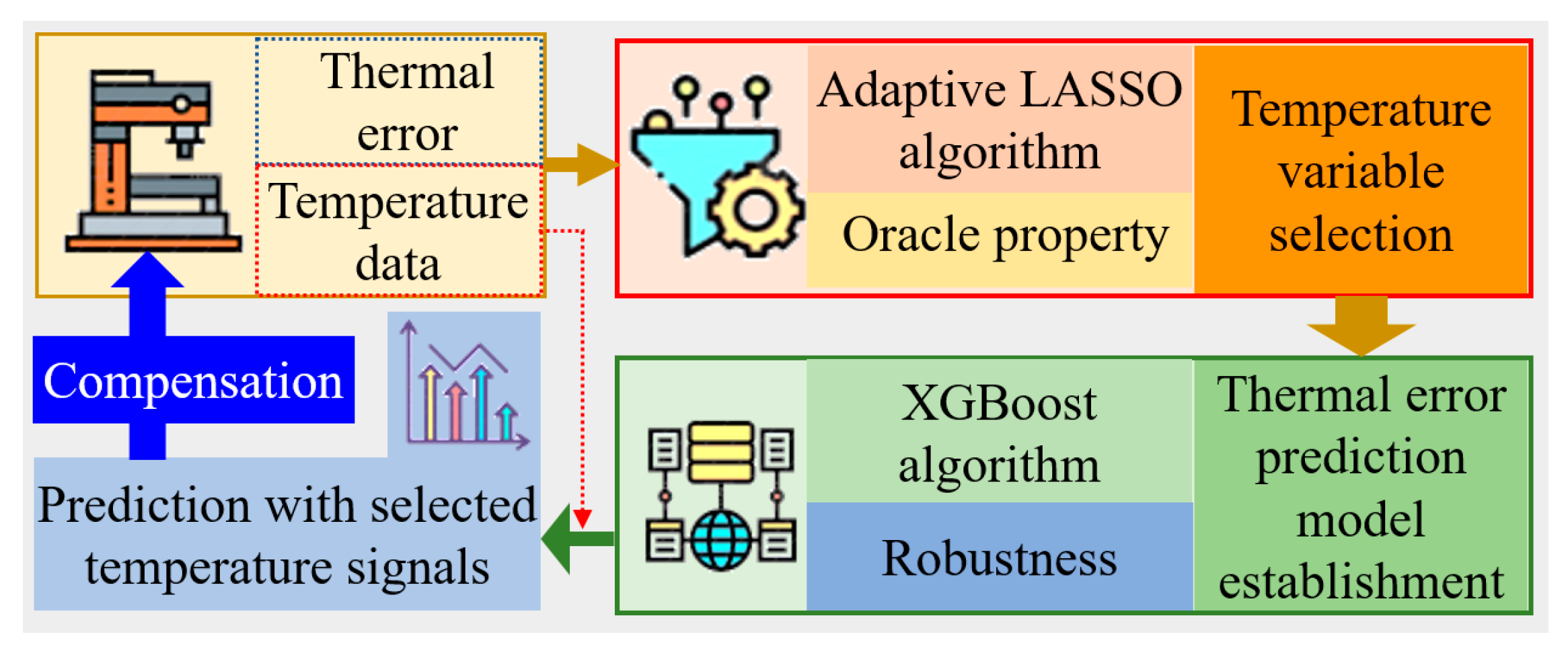
- The adaptive LASSO method enjoys the oracle property for selecting temperature-sensitive variables consistently; namely, it performs as well as if the true underlying model is given in advance. In addition, the adaptive LASSO method can be solved efficiently and achieves superior performance on variable selection in various applications.
- (2)
- The XGBoost algorithm is robust to multicollinearity in nature while the multicollinearity is commonly seen in thermal error modeling of CNC machines, and the embedded regularization in the XGBoost algorithm helps avoid over-fitting. In addition, different from existing neural network models which function as a black box and fail to interpret, the XGBoost method can provide desirable interpretable results and identify which variables have the most effects on thermal errors.
- (3)
- Both the adaptive LASSO and XGBoost algorithms are first-ever adopted in the literature to predict thermal errors for CNC machines. Our proposed method contributes to the practice of precision engineering by illustrating how practitioners can utilize the proposed method for accurate and robust thermal error predictions. Based on our experimental data from the Vcenter-55 type 3-axis vertical machining center, compared with several benchmark methods, the proposed ALIX algorithm demonstrates its superior performance in prediction accuracy, robustness, and worst-case scenario prediction.
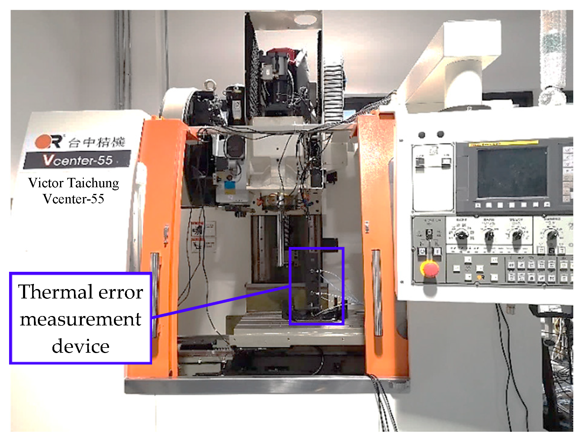
2. Thermal Error Experiment
2.1. Experiment Object
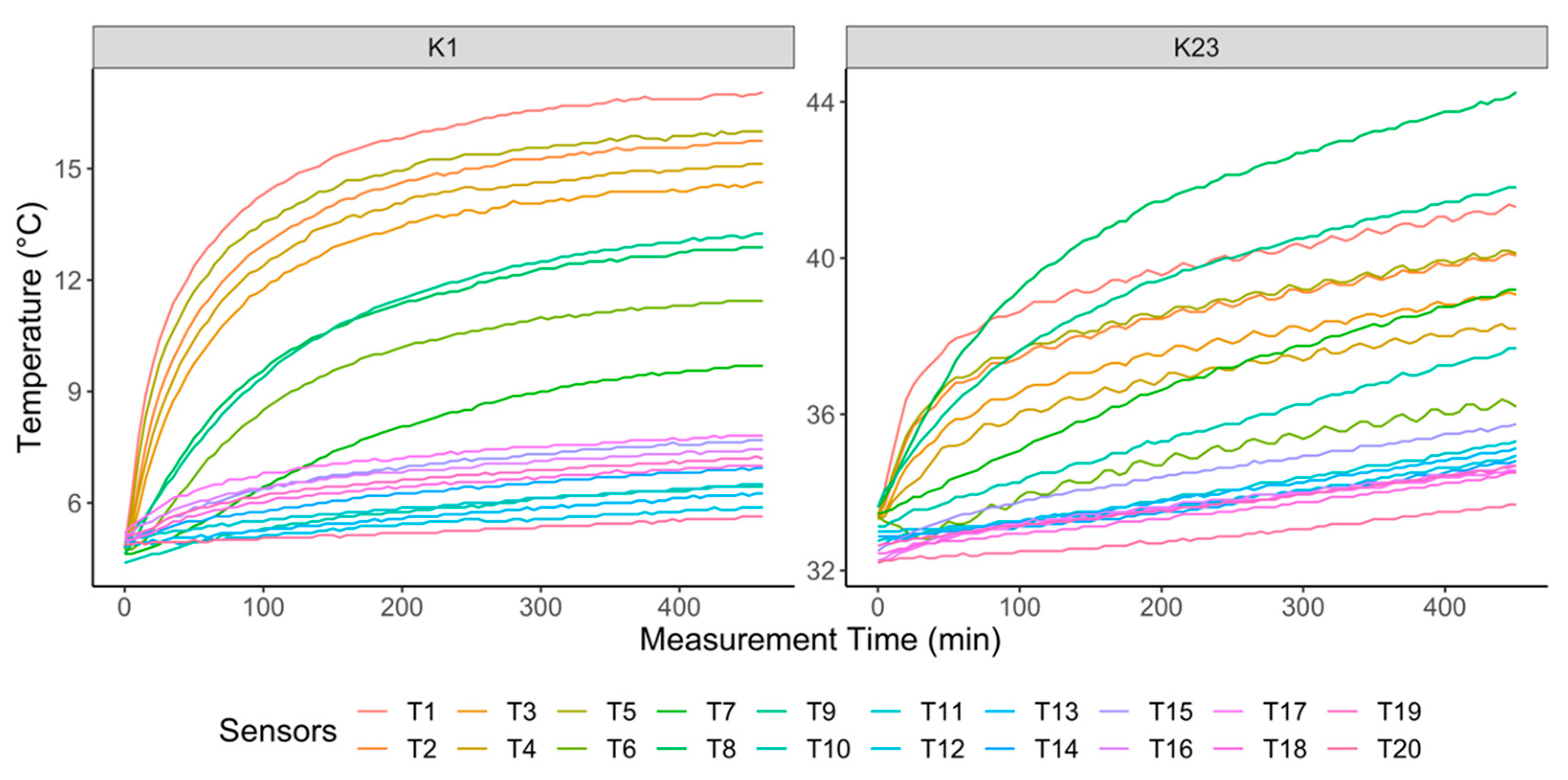
2.2. Exploratory Data Analysis
3. Methodology
3.1. Temperature-Sensitive Variable Selection
3.2. Thermal Error Modeling
4. Performance Evaluation
4.1. Temperature-Sensitive Variable Selection
4.2. Hyperparameter Setting and Interpretable Results
4.3. Performance Comparison
5. Experimental Verification
6. Conclusions
Author Contributions
Funding
Institutional Review Board Statement
Informed Consent Statement
Data Availability Statement
Conflicts of Interest
References
- Zimmermann, N.; Lang, S.; Blaser, P.; Mayr, J. Adaptive Input Selection for Thermal Error Compensation Models. CIRP Ann. 2020, 69. [Google Scholar] [CrossRef]
- Chiu, Y.C.; Wang, P.H.; Hu, Y.C. The Thermal Error Estimation of the Machine Tool Spindle Based on Machine Learning. Machines 2021, 9, 184. [Google Scholar] [CrossRef]
- Mayr, J.; Jedrzejewski, J.; Uhlmann, E.; Donmez, M.A.; Knapp, W.; Härtig, F.; Wendt, K. Thermal Issues in Machine Tools. CIRP Ann. 2012, 61, 771–791. [Google Scholar] [CrossRef] [Green Version]
- Creighton, E.; Honegger, A.; Tulsian, A.; Mukhopadhyay, D. Analysis of Thermal Errors in a High-Speed Micro-Milling Spindle. Int. J. Mach. Tools Manuf. 2010, 50, 386–393. [Google Scholar] [CrossRef]
- Xu, Z.Z.; Liu, X.J.; Kim, H.K.; Shin, J.H.; Lyu, S.K. Thermal Error Forecast and Performance Evaluation for an Air-Cooling Ball Screw System. Int. J. Mach. Tools Manuf. 2011, 51, 605–611. [Google Scholar] [CrossRef]
- Li, F.; Li, T.; Jiang, Y.; Wang, H.; Ehmann, K.F. Explicit Error Modeling of Dynamic Thermal Errors of Heavy Machine Tool Frames Caused by Ambient Temperature Fluctuations. J. Manuf. Process. 2019, 48, 320–338. [Google Scholar] [CrossRef]
- Thiem, X.; Kauschinger, B.; Ihlenfeldt, S. Online Correction of Thermal Errors Based on a Structure Model. Int. J. Mechatron. Manuf. Syst. 2019, 12, 49–62. [Google Scholar] [CrossRef]
- Naumann, C.; Glänzel, J.; Putz, M. Comparison of Basis Functions for Thermal Error Compensation Based on Regression Analysis—A Simulation Based Case Study. J. Mach. Eng. 2020, 20, 28–40. [Google Scholar] [CrossRef]
- Naumann, A.; Herzog, R. Optimal Sensor Placement for Thermo-Elastic Coupled Machine Models. PAMM 2021, 20, e202000255. [Google Scholar] [CrossRef]
- Świć, A.; Gola, A.; Sobaszek, Ł.; Šmidová, N. A Thermo-Mechanical Machining Method for Improving the Accuracy and Stability of the Geometric Shape of Long Low-Rigidity Shafts. J. Intell. Manuf. 2021, 32, 1939–1951. [Google Scholar] [CrossRef]
- Ramesh, R.; Mannan, M.A.; Poo, A.N. Error Compensation in Machine Tools—A Review: Part II: Thermal Errors. Int. J. Mach. Tools Manuf. 2000, 40, 1257–1284. [Google Scholar] [CrossRef]
- Liu, H.; Miao, E.; Wang, J.; Zhang, L.; Zhao, S. Temperature-Sensitive Point Selection and Thermal Error Model Adaptive Update Method of CNC Machine Tools. Machines 2022, 10, 427. [Google Scholar] [CrossRef]
- Liu, H.; Miao, E.; Zhang, L.; Tang, D.; Hou, Y. Correlation Stability Problem in Selecting Temperature-Sensitive Points of CNC Machine Tools. Machines 2022, 10, 132. [Google Scholar] [CrossRef]
- Yang, J.G.; Deng, W.G.; Ren, Y.Q.; Li, Y.S.; Dou, X.L. Grouping Optimization Modeling by Selection of Temperature Variables for the Thermal Error Compensation on Machine Tools. China Mech. Eng. 2004, 15, 478–481. [Google Scholar]
- Yan, J.Y.; Yang, J.G. Application of Synthetic Grey Correlation Theory on Thermal Point Optimization for Machine Tool Thermal Error Compensation. Int. J. Adv. Manuf. Technol. 2009, 43, 1124–1132. [Google Scholar] [CrossRef]
- Abdulshahed, A.M.; Longstaff, A.P.; Fletcher, S.; Myers, A. Thermal Error Modelling of Machine Tools Based on ANFIS with Fuzzy C-Means Clustering Using a Thermal Imaging Camera. Appl. Math. Model. 2015, 39, 1837–1852. [Google Scholar] [CrossRef]
- Liu, Y.; Miao, E.; Liu, H.; Feng, D.; Zhang, M.; Li, J. CNC Machine Tool Thermal Error Robust State Space Model Based on Algorithm Fusion. Int. J. Adv. Manuf. Technol. 2021, 116, 941–958. [Google Scholar] [CrossRef]
- Wei, X.; Miao, E.; Wang, W.; Liu, H. Real-Time Thermal Deformation Compensation Method for Active Phased Array Antenna Panels. Precis. Eng. 2019, 60, 121–129. [Google Scholar] [CrossRef]
- Zhang, T.; Ye, W.; Shan, Y. Application of Sliced Inverse Regression with Fuzzy Clustering for Thermal Error Modeling of CNC Machine Tool. Int. J. Adv. Manuf. Technol. 2016, 85, 2761–2771. [Google Scholar] [CrossRef]
- Miao, E.; Liu, Y.; Liu, H.; Gao, Z.; Li, W. Study on the Effects of Changes in Temperature-Sensitive Points on Thermal Error Compensation Model for CNC Machine Tool. Int. J. Mach. Tools Manuf. 2015, 97, 50–59. [Google Scholar] [CrossRef]
- Liu, H.; Miao, E.M.; Wei, X.Y.; Zhuang, X.D. Robust Modeling Method for Thermal Error of CNC Machine Tools Based on Ridge Regression Algorithm. Int. J. Mach. Tools Manuf. 2017, 113, 35–48. [Google Scholar] [CrossRef]
- Tan, F.; Yin, M.; Wang, L.; Yin, G. Spindle Thermal Error Robust Modeling Using LASSO and LS-SVM. Int. J. Adv. Manuf. Technol. 2018, 94, 2861–2874. [Google Scholar] [CrossRef]
- Fan, J.; Li, R. Variable Selection via Nonconcave Penalized Likelihood and Its Oracle Properties. J. Am. Stat. Assoc. 2001, 96, 1348–1360. [Google Scholar] [CrossRef]
- Zhu, M.; Yang, Y.; Feng, X.; Du, Z.; Yang, J. Robust Modeling Method for Thermal Error of CNC Machine Tools Based on Random Forest Algorithm. J. Intell. Manuf. 2022, 1–14. [Google Scholar] [CrossRef]
- Wei, X.; Ye, H.; Miao, E.; Pan, Q. Thermal Error Modeling and Compensation Based on Gaussian Process Regression for CNC Machine Tools. Precis. Eng. 2022, 77, 65–76. [Google Scholar] [CrossRef]
- Gao, X.; Guo, Y.; Hanson, D.A.; Liu, Z.; Wang, M.; Zan, T. Thermal Error Prediction of Ball Screws Based on PSO-LSTM. Int. J. Adv. Manuf. Technol. 2021, 116, 1721–1735. [Google Scholar] [CrossRef]
- Liu, J.; Ma, C.; Gui, H.; Wang, S. Transfer Learning-Based Thermal Error Prediction and Control with Deep Residual LSTM Network. Knowl.-Based Syst. 2022, 237, 107704. [Google Scholar] [CrossRef]
- Li, Z.; Zhu, B.; Dai, Y.; Zhu, W.; Wang, Q.; Wang, B. Research on Thermal Error Modeling of Motorized Spindle Based on Bp Neural Network Optimized by Beetle Antennae Search Algorithm. Machines 2021, 9, 286. [Google Scholar] [CrossRef]
- Liang, Y.C.; Li, W.D.; Lou, P.; Hu, J.M. Thermal Error Prediction for Heavy-Duty CNC Machines Enabled by Long Short-Term Memory Networks and Fog-Cloud Architecture. J. Manuf. Syst. 2020, 62, 950–963. [Google Scholar] [CrossRef]
- Liu, J.; Ma, C.; Gui, H.; Wang, S. Thermally-Induced Error Compensation of Spindle System Based on Long Short Term Memory Neural Networks. Appl. Soft Comput. 2021, 102, 107094. [Google Scholar] [CrossRef]
- ISO Copyright Office ISO 230-3 Test Code for Machine Tools Part 3: Determination of Thermal Effects 2020.
- Li, Y.; Zhao, W.; Lan, S.; Ni, J.; Wu, W.; Lu, B. A Review on Spindle Thermal Error Compensation in Machine Tools. Int. J. Mach. Tools Manuf. 2015, 95, 20–38. [Google Scholar] [CrossRef]
- Zou, H. The Adaptive Lasso and Its Oracle Properties. J. Am. Stat. Assoc. 2006, 101, 1418–1429. [Google Scholar] [CrossRef] [Green Version]
- Friedman, J.; Hastie, T.; Tibshirani, R. Regularization Paths for Generalized Linear Models via Coordinate Descent. J. Stat. Softw. 2010, 33, 1–22. [Google Scholar] [CrossRef] [PubMed] [Green Version]
- Friedman, J.; Hastie, T.; Höfling, H.; Tibshirani, R. Pathwise Coordinate Optimization. Ann. Appl. Stat. 2007, 1, 302–332. [Google Scholar] [CrossRef] [Green Version]
- Chen, T.; Guestrin, C. Xgboost: A Scalable Tree Boosting System. In Proceedings of the 22nd ACM SIGKDD International Conference on Knowledge Discovery and Data Mining, San Francisco, CA, USA, 13–17 August 2016; pp. 785–794. [Google Scholar]
- Friedman, J.H. Greedy Function Approximation: A Gradient Boosting Machine. Ann. Stat. 2001, 29, 1189–1232. [Google Scholar] [CrossRef]
- Kuhn, M. Building Predictive Models in R Using the Caret Package. J. Stat. Softw. 2008, 28, 1–26. [Google Scholar] [CrossRef] [Green Version]
- Miao, E.; Gong, Y.; Niu, P.; Ji, C.; Chen, H. Robustness of Thermal Error Compensation Modeling Models of CNC Machine Tools. Int. J. Adv. Manuf. Technol. 2013, 69, 2593–2603. [Google Scholar] [CrossRef]
- Wei, X.; Miao, E.; Liu, H.; Liu, S.; Chen, S. Two-Dimensional Thermal Error Compensation Modeling for Worktable of CNC Machine Tools. Int. J. Adv. Manuf. Technol. 2019, 101, 501–509. [Google Scholar] [CrossRef]


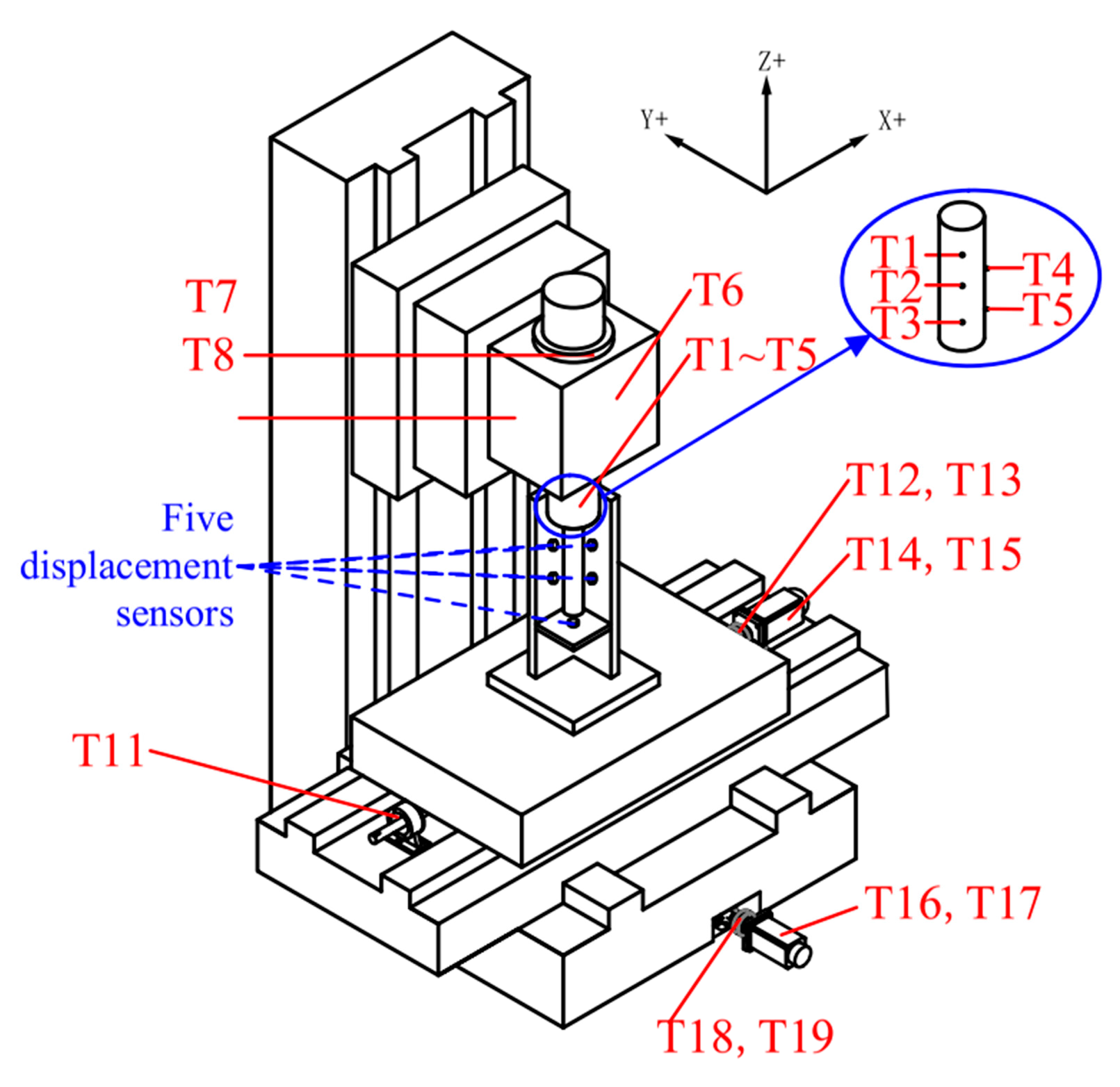
| Temperature Sensors | Installment Location |
|---|---|
| T1–T5 | Front bearing of the spindle |
| T6, T9 | Spindle box |
| T7, T8 | Spindle motor |
| T10 | Machine housing |
| T11 | Support base on X direction |
| T12, T13 | Screw nut on X direction |
| T14, T15 | Motor on X direction |
| T16, T17 | Motor on Y direction |
| T18, T19 | Screw nut on Y direction |
| T20 | Support base on Y direction |
| Batch | Spindle Speed (rpm) | Initial Ambient Temperature (Degree Celsius) | Batch | Spindle Speed (rpm) | Initial Ambient Temperature (Degree Celsius) |
|---|---|---|---|---|---|
| K1 | 4000 | 4.38 | K13 | 6000 | 10.88 |
| K2 | 4000 | 4.50 | K14 | 4000 | 12.94 |
| K3 | 4000 | 5.31 | K15 | 4000 | 14.44 |
| K4 | 6000 | 5.75 | K16 | 6000 | 14.63 |
| K5 | 6000 | 6.19 | K17 | 6000 | 21.69 |
| K6 | 4000 | 6.69 | K18 | 6000 | 24.50 |
| K7 | 6000 | 7.06 | K19 | 4000 | 25.06 |
| K8 | 4000 | 9.19 | K20 | 6000 | 25.63 |
| K9 | 4000 | 9.25 | K21 | 6000 | 25.69 |
| K10 | 4000 | 9.63 | K22 | 6000 | 27.75 |
| K11 | 6000 | 9.81 | K23 | 6000 | 33.13 |
| K12 | 6000 | 10.50 |
| Batch | Selected Temperature Sensors | Batch | Selected Temperature Sensors |
|---|---|---|---|
| K1 | 1, 3, 7, 11, 12, 13, 14, 16, 18, 19, 20 | K13 | 1, 2, 3, 7, 13, 14, 20 |
| K2 | 1, 11 | K14 | 1, 11, 20 |
| K3 | 1, 11, 14 | K15 | 2, 5, 7, 11, 20 |
| K4 | 1, 10, 12 | K16 | 2, 3, 5, 7, 11, 16, 20 |
| K5 | 1, 7, 10, 11, 17, 20 | K17 | 2, 3, 7, 11, 12, 13, 20 |
| K6 | 1, 10, 20 | K18 | 1, 3, 11, 19 |
| K7 | 1, 11 | K19 | 2, 6, 7, 8, 10, 11, 12, 13, 14, 16, 17, 18, 19, 20 |
| K8 | 1, 11 | K20 | 1, 8, 11 |
| K9 | 1, 3, 7, 10, 11, 17 | K21 | 1, 6, 7, 8, 10, 11, 16, 18, 20 |
| K10 | 1, 7, 11, 13 | K22 | 1, 3, 11, 12, 20 |
| K11 | 1, 10, 12, 13, 20 | K23 | 1, 8, 11 |
| K12 | 5, 12, 13, 14, 20 |
| Hyperparameters | Search Space |
|---|---|
| number of iterations | {500, 1000} |
| maximum depth | {4, 6} |
| eta | {0.01, 0.05} |
| minimum child weight | {0, 20} |
| gamma | {0, 50} |
| Method | OLS | LASSO-SVM | RF | ALIX |
|---|---|---|---|---|
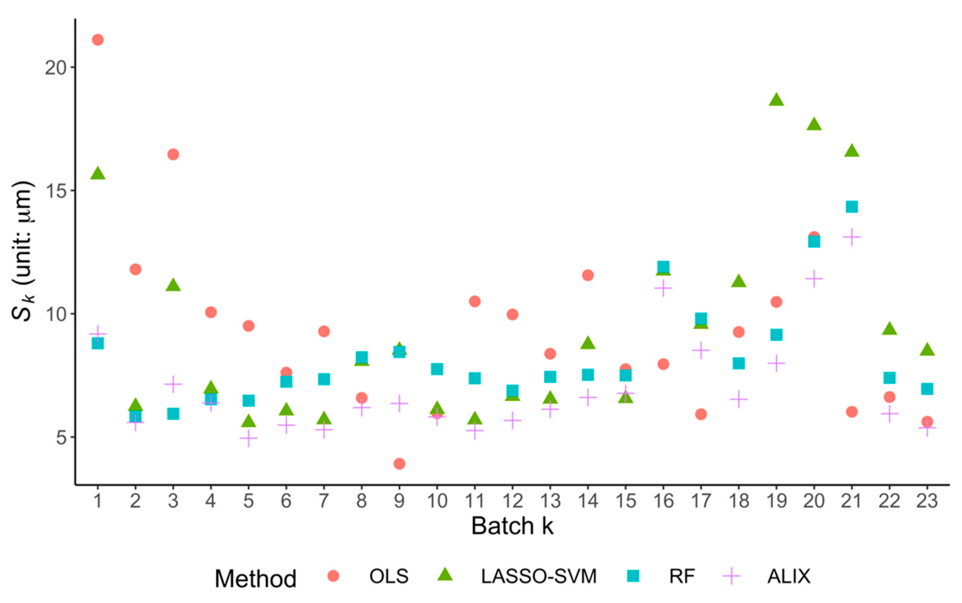
| (unit: ) | 9.37 | 9.42 | 8.25 | 7.05 |
| (unit: ) | 7.02 | 7.07 | 6.44 | 5.61 |
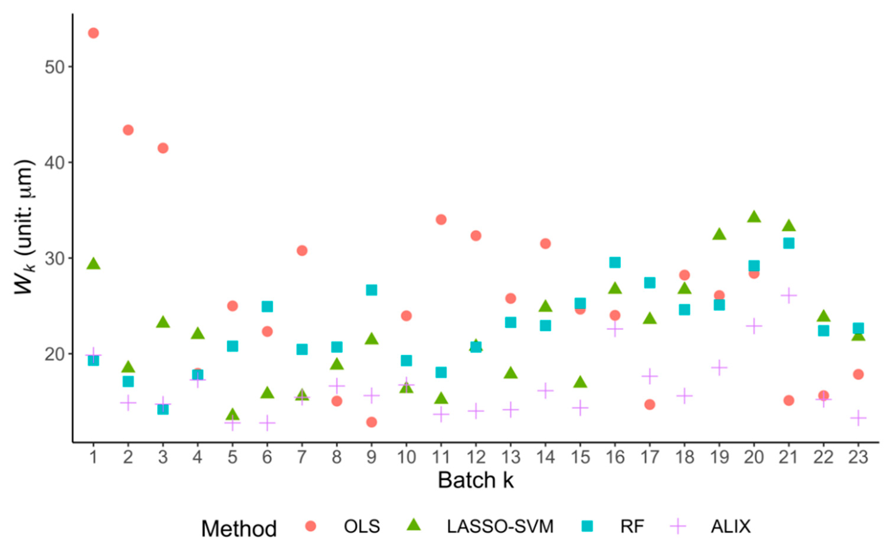
| (unit: ) | 26.29 | 22.00 | 22.78 | 16.49 |
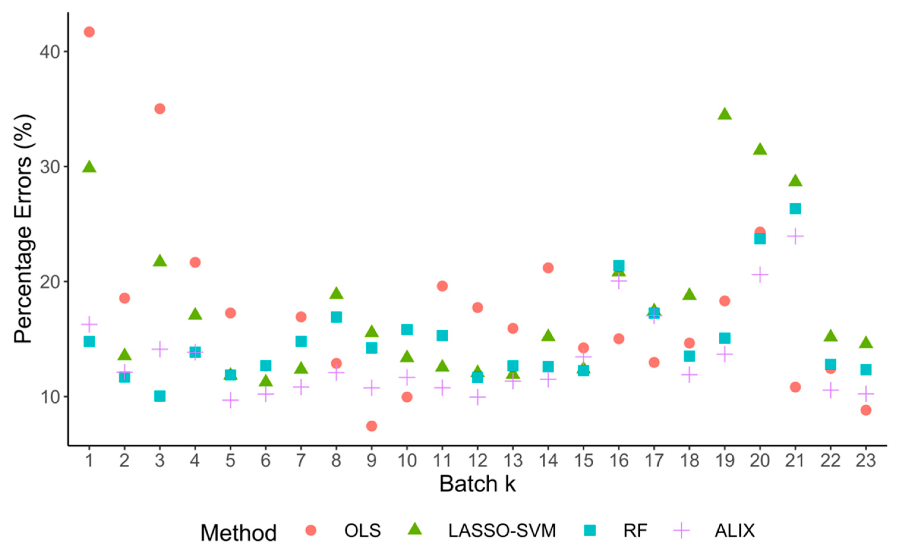
| (unit: %) | 17.39 | 17.86 | 14.94 | 13.33 |
Publisher’s Note: MDPI stays neutral with regard to jurisdictional claims in published maps and institutional affiliations. |
© 2022 by the authors. Licensee MDPI, Basel, Switzerland. This article is an open access article distributed under the terms and conditions of the Creative Commons Attribution (CC BY) license (https://creativecommons.org/licenses/by/4.0/).
Share and Cite
Ye, H.; Wei, X.; Zhuang, X.; Miao, E. An Improved Robust Thermal Error Prediction Approach for CNC Machine Tools. Machines 2022, 10, 624. https://doi.org/10.3390/machines10080624
Ye H, Wei X, Zhuang X, Miao E. An Improved Robust Thermal Error Prediction Approach for CNC Machine Tools. Machines. 2022; 10(8):624. https://doi.org/10.3390/machines10080624
Chicago/Turabian StyleYe, Honghan, Xinyuan Wei, Xindong Zhuang, and Enming Miao. 2022. "An Improved Robust Thermal Error Prediction Approach for CNC Machine Tools" Machines 10, no. 8: 624. https://doi.org/10.3390/machines10080624