Article

A Quantile Dependency Model for Predicting Optimal Centrifugal Pump Operating Strategies

1
Department of Electronic and Electrical Engineering, University of Strathclyde, Glasgow G1 1XW, UK
2
Alan Turing Institute, British Library, London NW1 2DB, UK
*
Author to whom correspondence should be addressed.
Machines 2022, 10(7), 557; https://doi.org/10.3390/machines10070557
Submission received: 30 May 2022 / Revised: 1 July 2022 / Accepted: 3 July 2022 / Published: 10 July 2022
(This article belongs to the Special Issue Fault Diagnosis and Health Management of Power Machinery)

Abstract

:
Used in many industrial applications, centrifugal pumps have optimal operating criteria specified at design. These criteria may not be precisely adhered to during operation which will ultimately reduce the life of the asset. Operators would therefore benefit from anticipating how often the design point is deviated from and hence how much asset degradation results. For centrifugal pumps, a novel set of covariates were proposed in this paper which formally partition observed operating zones with an Empirical Bivariate Quantile Partitioned distribution. This captured the dependency relation between operating parameters across plant configurations to predict the component wear that results from particular settings. The effectiveness of this was demonstrated through an operational case study in civil nuclear generation feedwater pumps where corroboration with bearing movements provides an indicator of plant wear. Such a technique is envisaged to inform operators of optimal plant configuration from multiple possibilities in advance of undertaking them.

1. Introduction

Generation margins in conventional thermal power stations can be threatened by unexpected plant outages caused by sudden equipment failure. This has motivated more intensive monitoring of critical plant assets to forestall this, however, in many cases plant configuration plays a role in the rate of plant aging or performance deterioration. For rotating plant assets in nuclear stations, extensive monitoring is routine [1] and generally involves quantifying deviations from expected sensor values and their thresholds for alarm and halt limits. With many civil nuclear generation facilities now passing their original operational lifetimes, ref. [2] notes that lifetime extension could be justified on the basis of greater situational awareness of critical plant assets and the degradation processes they face. While design stage knowledge may inform hard limits for observed sensor values, the operational consequence may not always be apparent. While design stage knowledge may inform hard limits for observed sensor values, the operational consequence may not always be apparent, motivating a means of relating the plant operating regime to the operational consequence to show how the physical system responds [3,4]. The term inferential sensing refers to the case whereby quantities of interest in a system can be inferred from other correlated or dependence measurements from sensors [5]. These dependent operating values can be anticipated in a number of ways [6]: via detailed physics models, models driven through high-level knowledge in the form of rules or heuristics, and data-driven models. However, the required inputs and modelling assumptions that would drive these predictions are not always going to be clear to the plant operators, which necessitates a data-centric approach. Recovering relations between operating conditions and expected asset response from monitoring data would amount to model inversion, commonly used for anomaly detection [7,8], but a key drawback is that a poorly specified model may produce incorrect outputs for inputs in certain ranges or perturbations, which in turn would misinform how the plant should be operated [9]. Additionally, [10] identified that condition monitoring data may not exist in large enough volumes or with extensive plant coverage, meaning a universal approximation approach, such as Deep Learning, may not be practical. To mitigate the problem of model misspecification, predictions from a number of diverse models may need to be taken into account in a principled manner [11,12].
Commonly used in many industries [13] and the focus of this paper, centrifugal pumps are specialized cases of rotating plant in that the working fluids’ characteristics can change with the operating parameters of the plant, which in turn can affect its condition. Centrifugal or rotodynamic pumps are key components in nuclear generation station designs [14], being used to provide coolant or feed water to boilers and in many cases have bespoke design refinements optimizing their performance to a particular site. This can make constructing physics-based models time-consuming through the lack of opportunity for generalization across assets.
The purpose of this paper was to present a data-driven approach to quantify the impact of operational decisions that place a rotodynamic pump outside its preferred zone of operation. The challenge in undertaking this is in correctly identifying a measure of instantaneous plant health and forming the relation between this and the operating parameters of the plant. To address this, the contribution of this paper is to produce a novel set of covariates by formally partitioning observed operating zones using an Empirical Bivariate Quantile Partitioned distribution [15], which captures the dependency relation between the pump operating parameters across all regions of normal operation and then uses these as regressors to predict the component wear that results from particular operating settings. The complex form of the relation is addressed with an ensemble machine learning approach to provide accurate prediction through the complete range of operational settings. The benefit of this contribution to the plant operator is twofold: prospective operating scenarios can be tested with the relational model to anticipate the consequence incurred in plant health; previous operational decisions can be retrospectively assessed in terms of their consequence. Both benefits allow plant operators to identify operational schedules that are optimal for minimizing component wear and therefore extending plant service intervals and lifetime.
The paper is organized as follows: Section 2 provides an overview of the operation and application of centrifugal pumps with a specific example of boiler feeds in a nuclear generation; Section 3 reviews the concept of the pump curve in pump design and operation, how this relates to condition monitoring data gathered by operators and how its characteristics may be generalized through analytical tools and used in this paper as model covariate inputs; Section 4 sets up the protocol for using covariate generalizations as inputs to a variety of predictive models of plant degradation. Section 5 applies this novel concept against real operational data and benchmark model inputs. Finally, in Section 6 the authors outline the main operational use case envisaged for an industry deployment of the contribution.

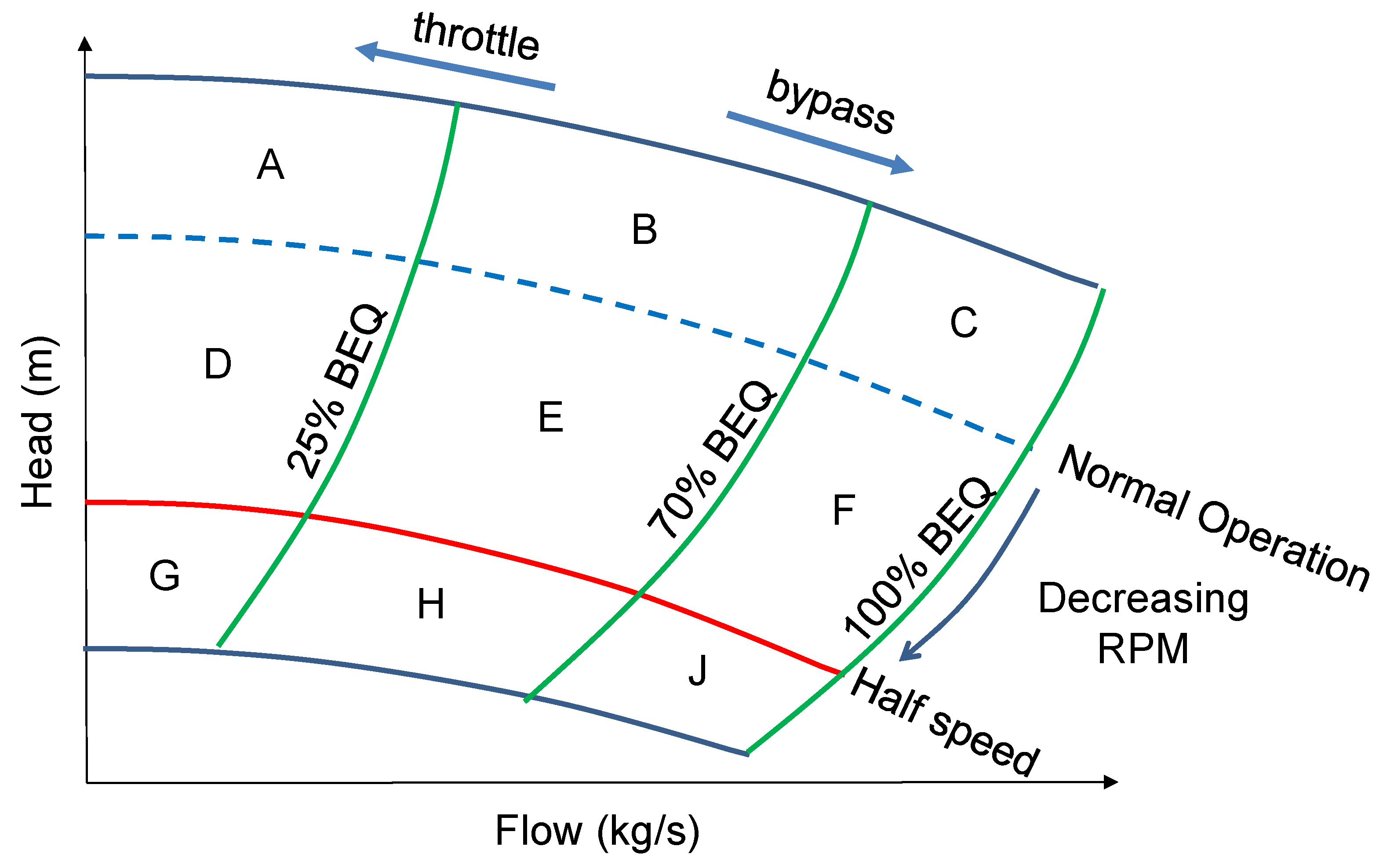
2. Centrifugal Pumps: Principles of Operation and Industrial Application

Rotodynamic or centrifugal pumps have applications across a number of industries including conventional thermal generation, pumped storage, mining, marine, and domestic utility [13,16]. While each of these applications will utilize a pump with an operating range designed for their respective application, there will still be best efficiency points in this range that will minimize losses through vibration. Centrifugal pumps are generally operated according to a pump curve [16]—a relation between head and flow that captures its full operational range and specifies the most efficient operating point(s). The relation between the head and flow pairings that result in optimal pump operation vary according to the rotating speed of the pump. Combinations of these pairings can also be detrimental to the plant’s useful life, so plant operators have a particular approach to operating pumps with regions being visited according to operational settings. Figure 1 highlights examples of what these broadly might be.
Throttling the flow (through closing an inlet valve for example) results in a reduction in flow for a constant operating speed—various Best Efficiency flow (BEQ) values are shown in Figure 1. Similarly, reducing the speed will reduce both flow and head. Although optimal operation pump curve locations are specified by the Original Equipment Manufacturer (OEM), operators may not always adhere exactly to this guidance, and remaining on, or finding operational settings that attain the exact duty point may be difficult, so in practice, a close neighborhood is sought instead. This relative deviation will affect the pump’s health and how it performs.

Case Study: AGR Main Boiler Feed Pumps

Boiler feed pumps provide the pressure difference and resultant flow required to translate water from condensers to the shell side of the primary heat exchanger or boiler in many power stations [14]. There is often a booster pump located upstream of the boiler pumps to overcome the negative gauge pressure in the condensers during normal operation [17]. Also, there are often heating stages downstream of the boiler pumps between the boiler pumps and the boiler—the pressure increase produced by the boiler pumps must therefore also overcome any pressure restriction realized by these components/restrictions which can be an additional contributing factor to their performance and health.
In the UK, the Advanced Gas-cooled Reactor (AGR) design dominates civil nuclear generation and features two turbine-driven Main Boiler Feed Pumps (MBFP—Figure 2) [14]. As the continued flow of fluid in the water-steam cycle of a power station is critical to its continued operation and electrical generation [18] it is imperative that boiler pumps are monitored for any abnormal behavior or phenomenon that may contribute to accelerated plant degradation or to tripping the plant which would result in reduced or zero power generation. Monitoring of various parameters is accounted for during station design and construction and hence can generally be monitored independently and without causing obstruction to generation. Ref. [19] (Table 1) gives a high-level overview of some critical rotating machines (and component parts) that are monitored, why they are monitored and the techniques and algorithms that are commonly adopted to conduct diagnostic and prognostics tasks.

3. Pump Curve Quantile Characterization

The rotating plant operating regime plays a dominant role in its vibration and performance indicators; often movement between these regimes is when changes in these indicators occur. One of the challenges of accommodating expected operational state changes is identifying the associated signatures and bounds of these regimes and obtaining markers of where they begin and end. Producing a useful representation of non-stationary rotodynamic pump operation requires exemplar data to be treated according to the plant’s operating state. Failure to do this will result in behavior from two or more operating states being merged into a single unrepresentative state that offers no guidance to the operator as to the positioning and variation of operational bounds. The following sections document the proposed approach to identifying this data automatically, defining the space over which it is modelled, proposing a means of accurately capturing its variability, and, with these in place, defining a measure of how far from the optimal operation the plant has moved.

3.1. Automatic Operating Zone Delineation

For an MBFP in an AGR, the following station regimes result in a change in performance that has been seen to influence vibration and performance measurements [1,20]: Refueling, Offline, and Online/Normal Operation. A feature of the AGR design is that it can be refueled while still generating, albeit on reduced power. A measurement that is a reliable indicator for these operating regimes or states is the MBFP rotational speed. The normal operating state value for this is station specific while the offline value is zero. While simple rules could be used to segment the operational regimes, the transitional behavior, operational noise and operational artefacts (such as those that occur during refueling) can make it difficult to define robust bounds.
Figure 3 shows the frequency of occurrence of the different rotational speeds a pump experiences over the course of a year. Although modes are evident in Figure 3, it is not clear where their bounds lie. Segmentation driven by operational data provides an alternative to this: a model can identify dominant modes of operation within indicator variables (pump speed or a feature vector derived from pump speed) and then use this as a measure of ‘soft evidence’ of a change in regime [21,22]. Although based on time series data, this process is not dissimilar to clustering. Since the plant’s operational state is never actually observed, the process is a hidden one—a hidden first-order Markov model or chain. A Hidden Markov Model (HMM) can be learned from a set of noisy observations and the resulting model can be used to recover a state sequence best representative of the stochastic process that generated it. In our case, we assume that the HMM can be in one of M unobserved states with transitions between states specified by a mixing matrix A in RMxM. In the ith state, the observations are assumed to be independent and follow a Gaussian distribution N(μi, σ2i). The emission model parameters must also be inferred from the data and the size of M, or the number of modes, can be estimated via a formal model order selection criteria such as AIC or BIC [23].
The challenge associated with fitting such an HMM to data is threefold. (i) Given the model parameters and observed data, estimate the optimal sequence of hidden states; (ii) given the model parameters and observed data, calculate the model likelihood; (iii) given the observed data, estimate the emission parameters. The first two challenges can be addressed using the Viterbi algorithm [24], while the last problem is typically solved using Expectation Maximization, known in this context as the Baum-Welch algorithm [25].
This model is functionally equivalent to fitting a Gaussian mixture model with M components and mixing weights pi. Employing this model selection strategy to a full year of MBFP rotational speed data identifies five distinct operating modes corresponding to the states in the Gaussian Mixture Model as shown in Figure 4.
Using the trained model on an out-of-sample rotational speed data set is shown in Figure 5. From Figure 4 and Figure 5, it is clear that offline states have been identified as State #5 while refueling is State #3 and normal operation is State #1 and #2. With the state of the station identifiable for every time step, this latent indicator can be used to segment the condition monitoring data stream allowing each operating state to be considered separately.

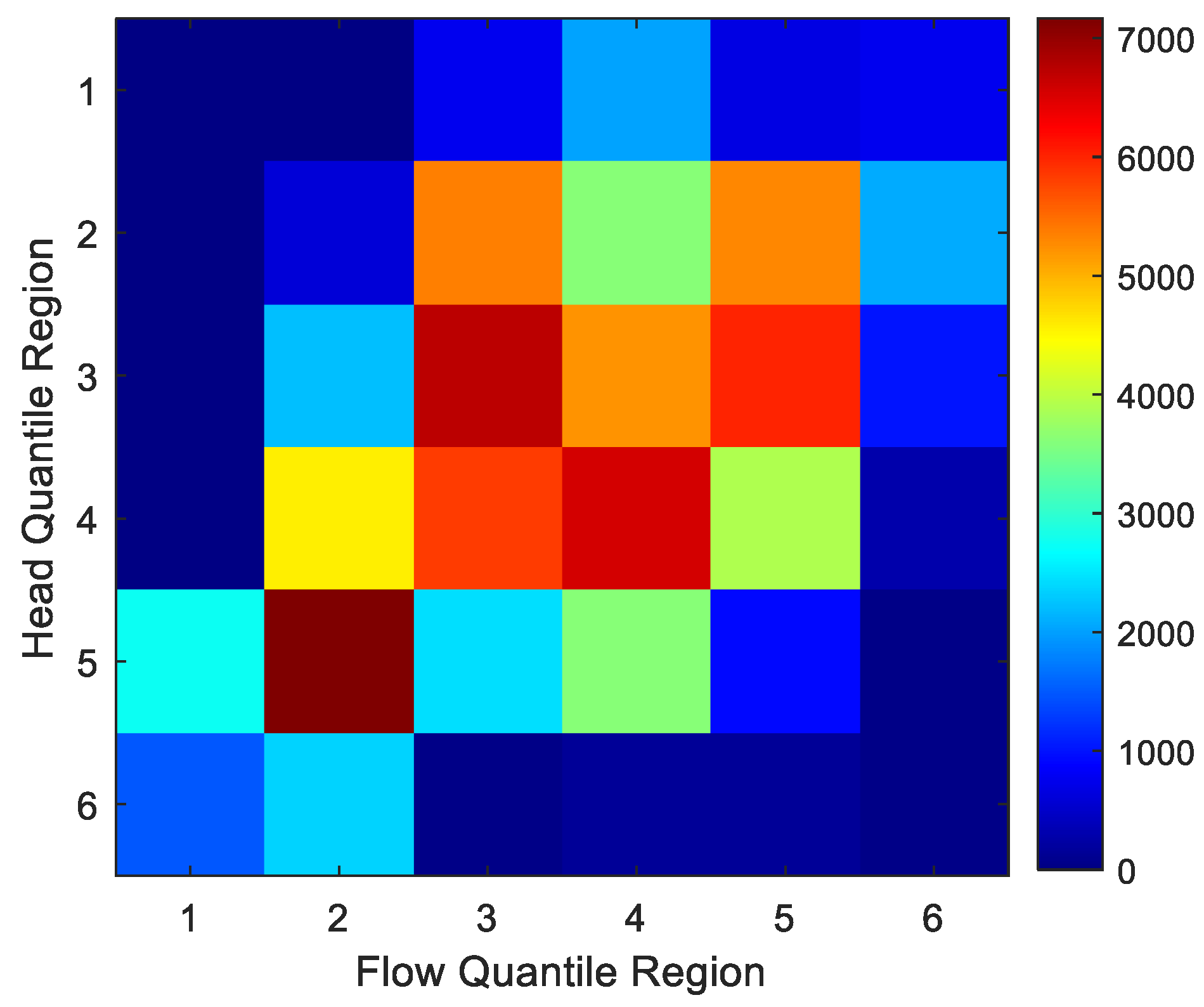
3.2. Empirical Bivariate Quantile Partition: Quantification of Preferred Operation Adherence

The consequence of operation at the extremes of the pump curve is known to cause particular modes of performance deterioration, so the hypothesis behind this model is that occurrences of operation within these regions (captured as counts) will result in a particular rate of performance deterioration. Figure 6 shows the flow and head relations for a year of pump operation after the non-normal operational states have been removed using the HMM approach described in Section 3.1.
While normal operation requires a constant rotational speed, there is clear variation evident within this plant state from Figure 6. What is not evident is the duration spent in each region. To provide a quantitative measure, it is proposed that an Empirical Bivariate Quantile Partitioned (EBQP) distribution [15] be used, where empirical quantiles of the marginal distributions form partitions in a contingency table-like dependency structure [26]. This is useful in this case as it does not enforce an assumption of correlation between flow and head variables in the various pump curve regions, and permits tails to behave in a different manner to those around the joint median. In an EBQP for this application there will be a bivariate sample of flow Q and head P at time t:
( Q t , P t )   t = 1 T  
The joint cumulative distribution F(q, p) has marginal distributions G(q) and H(p) and can be estimated as
F ^ ( q , p ) = 1 T t = 1 T I { Q t q , P t p }
and G ^ and H ^ defined analogously. The marginal distributions Q and P are discretized along a mesh 0 = γ0 < γ1 < ⋯ < γr = 1 and 0 = η1 < η2 ⋯ < ηc = 1, respectively. Here, the following set is used to capture more detail at the extremities:
γ = η = { 0 , 0.05 , 0.25 , 0.5 , 0.75 , 0.95 , 1 }
with
γ 0 = η 0 = 0
γ r = η c = 1
The marginal counts will be determined by the inverse empirical CDFs for Q and P respectively:
u i = inf { u : γ i G ^ ( u ) }
v i = inf { v : η i H ^ ( v ) }
for i = 1, …, r and j = 1, …, c. Together, this gives a joint count of
λ i j = F ^ ( u i , v j ) F ^ ( u i 1 , v j ) F ^ ( u i , v j 1 ) + F ^ ( u i 1 , v j 1 )
From (8), a vector Λ, counting how long the pump spends in each region will give an analogous measure to the wear that would be experienced in an equivalent region of the pump curve—a representation of this is shown in Figure 7.
Looking at how the 36 counts grow in each region individually shows the regions that are never visited and those that are visited only at certain times of year—this is shown in Figure 8 which takes the same count data shown in Figure 7 and presents it as it accumulates over time.
Figure 8 highlights that some regions are not revisited for months on end while some rise continually throughout the year of operation. Domain expertise (captured generally in [13]) notes that lengthy periods spent in particular regions are harmful to the pump asset, so increasing counts reflecting operating in these specific regions will in turn have an impact on the condition of the pump.

3.3. Measuring Operational Consequence: Choice of Degradation Metric

Having proposed a means of articulating a chosen operational strategy, the remaining part of the contribution is to select an observation that quantifies the consequence of this strategy. Component wear is synonymous with plant degradation, which will ultimately manifest in the statistical characteristics of operational data [8]. A thrust bearing is a standard component in pump design, which prevents axial movement along the length of the shaft during operation. If the pump experiences an excessive axial force this will lead to the thrust bearing pads deteriorating faster than expected and can lead to failure (via shaft seizure) without a maintenance intervention [27]. Axial forces result in both directions during both normal and abnormal pump operational conditions thus motivating the choice of the thrust bearing movement as the degradation metric for the MBFP with consequence being in proportion to bearing movement. Vibration levels cannot reliably be used owing to multiple operating states resulting in differing rotational speeds, which may not necessarily lead to a consistent indicator of wear. To provide an element of memory of operational extreme, the thrust bearing movement median observed over an hourly basis and a daily basis are considered, albeit separately, in order to identify the ideal resolution of model operation.

4. Pump Performance Response Quantification

The high dimensional multivariate input and the potentially nonlinear relation with the observed plant degradation make this challenging for many regression models [28], particularly when there are multiple operating regimes [29]. This section will therefore highlight the strategy used for constructing this functional form and its corresponding inputs, for maximally accurate performance estimates.

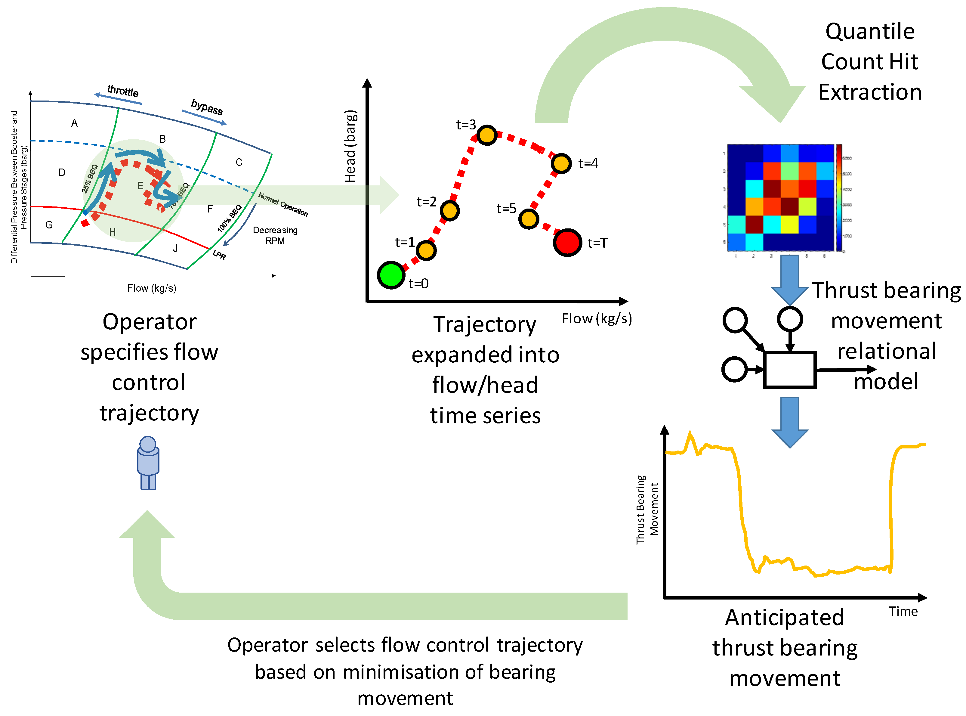
4.1. Relational Model—Operation/Thrust Bearing Movement

A number of different Machine Learning regression models are employed to capture the relation between the pump operational characteristics and the condition variable, the thrust bearing movement. The models used were chosen so that the limitations of the regression method and its underlying optimization of parameters would not obscure the predictive quality of the input features. These have been selected as:
  • Ordinary Least Squares linear regression (Models 1–3)
  • Least Squares and Absolute Shrinkage Selection Operator (LASSO) (Models 4–6)
  • Random Forest Regression, learning rate 1.0, LSBoost, 100 tree learners, (Models 7–9)
  • Tree Regression with pruning and leaf merging (Models 10–12)
  • Support Vector Regression with linear kernel (Models 13–15)
  • Gaussian Process Regression with a squared exponential kernel with parameters set to be the lengthscale and the standard deviation of the training data (Models 16–18)
Employing these regression models with their parameters estimated from an exemplar 6 months of data allows the thrust bearing movement for the subsequent periods of time to be estimated for a given operating strategy.

4.2. Candidate Inputs

For the purposes of comparison of the input feature predictive power with the simplest base case, the raw pump measurements, three sets of model inputs have been chosen as listed in Table 1.
Three sets of covariates are utilized: the first comprises the flow and head-direct observations from the pump curve. The second supplants the pump curve observations with cumulative hit counts obtained from each of the 36 regions of the EBQP. This second set of covariates is intended to capture the known consequences of operating with particular head/flow combinations as the dependency expressed through the EBQP. Several regression models will now be utilized to relate the movement of the thrust bearing to particular operating settings.

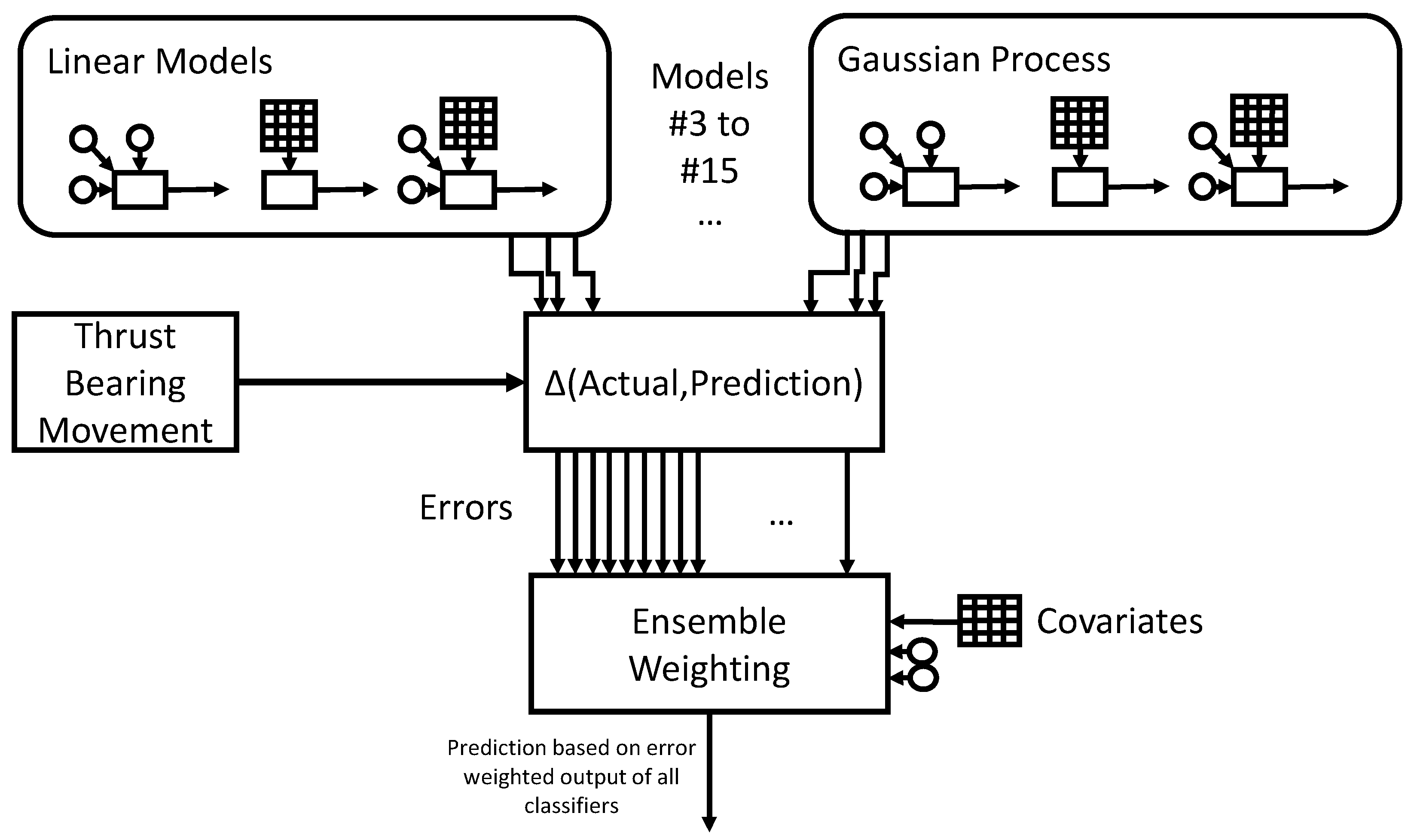
4.3. Ensemble Predictions

Given the dynamics and the operational extremes of pump operation, it is inevitable that no single regressor will provide high performance over the whole operating range of a pump. The need to avoid the as yet unknown performance limitations of any given regression model motivates the use of an ensemble for model predictions.
Figure 9 shows the complete model with the three covariate sets and the six predictive models, resulting in an 18-input ensemble. Two strategies are used for combining these 18 model outputs into a single optimal prediction: simple averaging of the constituent N model predictions and Pseudo Bayesian Averaging [30]. The prediction from the simple ensemble of N predictors amounts to
Y ^ = 1 N i = 1 N y ^ i
The Pseudo Bayesian approach uses the following weighting of the constituent predictions
Y ^ = i = 1 N w ^ i y ^ i
where the weights w are found from model prediction errors ε over sample size T:
w k = e x p ( t = 0 T ε k t ) i = 1 N e x p ( t = 0 T ε i t )
The weights are found from the in-sample data used to learn how much the constituent predictive models should contribute to the predictions out-of-sample.

4.4. Performance Measures

Considering how this model would be used in practice, there are two perspectives on model prediction accuracy: A binary one where the thrust bearing is predicted to move or not; and a real valued one where the magnitude and direction of the bearing movement are predicted. The latter is considered by plant operators to be more important as it offers not just the immediate consequence of plant maloperation but also a measure of wear on components [27].

5. Evaluation of Proposed Operations by Predicting Resultant Degradation

In order to test the predictive effectiveness of the pump operation features with respect to plant bearing wear, one year of operational data for a single unit was selected. This data comprised 5 min sampled bearing movements as well as pump speed, flow, and inlet and outlet pressure measurements that permitted the calculation of head. These performance parameters were sampled at 10 min intervals. The pump speed was used to obtain the regimes for the pump operation as outlined in Section 3 and separate normal operation from refueling operations or shutdowns.
Two investigations were carried out to understand the sustained effect of maloperation of the pump which resulted in the formation of two data sets: aggregated measurements over a 1 h period which comprised averaged pump performance parameters and cumulative quantile region counts being related to a maximum thrust bearing movement. The same observations were used for the second test only at day-level aggregation. A six-month period of operation was used to learn the relation between the pump curve and the thrust bearing movement and then tested on another 6 months of sample data. This is motivated by the need to keep training data requirements to a minimum. Each of the 18 (combinations of the six models and three input sets) predictors were then learned for both the hourly and daily aggregations.
Table 2 and Table 3 summarize the overall errors in terms of Mean Absolute Error (MAE). All models except the OLS regression utilize some kind of parameter selection meaning that uninformative inputs are minimally weighted. This rules out certain quantile hit counts to the detriment of some models (e.g., Random Forrest on all covariates) and to the benefit of others (e.g., tree on the proposed quantile counts). For the daily predictions, this has a knock-on effect for the ensembles with many individual models outperforming the averaged and weighted averaged predictions. In all four cases, the overall performance benefit is from the covariate set proposed rather than from the model. For hourly aggregations, the Ensemble models have the lowest MAE using the combined covariate sets. For daily operation, the hit counts alone offer a better prediction of consequence with an error of only 0.003 μm.

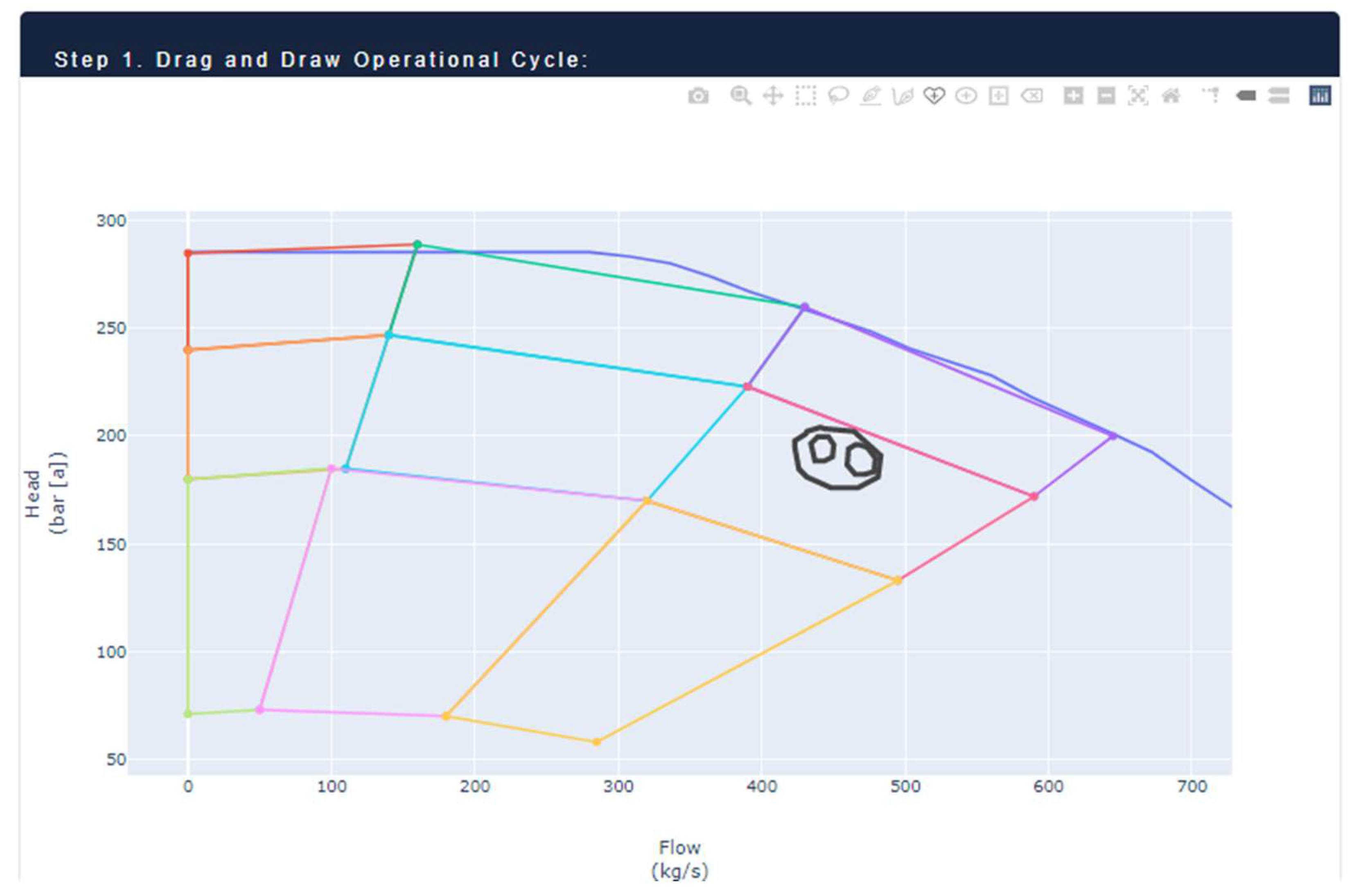
6. Operational Use Case

Where this modelling strategy is expected to provide value operationally is in the prediction of harmful operating regimes ahead of them actually being entered. To this end, a basic maloperation prediction model is embedded within a user interface to allow operators to plan operational trajectories within the confines of the pump curve. Figure 10 shows a schematic of where this tool would fit within the workflow of a plant operator.
Ahead of starting the pump or transitioning between operating regimes, the operator could plan several flow control settings as indicated in Figure 10. The proposed model allows a translation of these flow settings (with appropriate durations) into plant health consequence predictions.
For practical station deployment, this functionality would need to be driven by a graphical interface for use with plant operating personnel. Such a decision support system can allow the prediction of operational consequences as described, but also enables retrospective analysis of past operations which will grow supporting domain knowledge on the configuration preference of the plant being operated.
Figure 11, Figure 12, Figure 13 and Figure 14 show this user interface. In Figure 11 the operator draws a trajectory through the pump curve representing the flow and head levels obtained from a particular operational setting. Figure 12 shows how these three trajectories translate into flow and head time series, which in turn are used to predict the operational consequence in terms of thrust bearing movement time series in Figure 13. The table in Figure 14 highlights the cumulative bearing movement and hence the lowest operational consequence. It would be anticipated that the operator referenced this before carrying out the chosen operating strategy.

7. Conclusions

Generation plant reliability will continue to require the attention of asset owners and power industry stakeholders as the run-down of thermal type generation plant challenges the security of supply concerns at national scales. Operating plant optimally has the potential to increase service intervals and extend asset lifetimes. This paper has presented a means of automatically quantifying the asset health benefit of remaining within manufacturer-specified operating bounds based on well-understood performance measures. While this could be undertaken through a digital twin type approach, the efforts required in gathering understanding and devising a physics-based model for the replication of all possible behaviors are beyond the practical and resource constraints of most generation operators. For a unique generation asset, like the pumps used in the given case study, the operational benefit would be questionable. Instead, identifying general consequence has been achieved through the application of diverse predictors, combined with ensemble regression without the need for complex physics models or unrealistic high-resolution data. For operators, it is envisaged that pump set point planning would be an initial application of the proposes approach with movement through the curve chosen on a schedule then run through the model to identify a consequence ahead of application. Multiple candidate operating strategies can be trialed and ranked to find the optimal, although longer term this could form criteria for automated scheduling.

Author Contributions

Conceptualization, B.S. and B.B.; methodology, B.S., H.H.-H. and A.D.; software, B.S., H.H.-H., A.D., A.Y. and B.B.; validation, B.S., A.D. and B.B.; formal analysis, B.S.; investigation, B.S. and B.B.; data curation, B.S. and A.Y.; writing—original draft preparation, B.S.; writing—review and editing, B.S., B.B., A.Y., A.D., S.D.J.M., G.W. and C.M.; visualization, B.S.; project administration, B.B.; funding acquisition, S.D.J.M., C.M. and G.W. All authors have read and agreed to the published version of the manuscript.

Funding

This research was funded by Engineering and Physical Sciences Research Council, grant number EP/R004889/1 “Delivering Enhanced Through-Life Nuclear Asset Management”.

Institutional Review Board Statement

Not applicable.

Informed Consent Statement

Not applicable.

Data Availability Statement

Not applicable.

Conflicts of Interest

The authors declare no conflict of interest. The funders had no role in the design of the study; in the collection, analyses, or interpretation of data; in the writing of the manuscript, or in the decision to publish the results.

References

  1. Garvey, J.; Garvey, D.; Seibert, R.; Hines, J.W. Validation of on-line monitoring techniques to nuclear plant data. Nucl. Eng. Technol. 2007, 39, 149–158. [Google Scholar] [CrossRef] [Green Version]
  2. Coble, J.; Ramuhalli, P.; Bond, L.J.; Hines, J.; Ipadhyaya, B. A review of prognostics and health management applications in nuclear power plants. Int. J. Progn. Health Manag. 2015, 6, 16. [Google Scholar]
  3. La Roche-Carrier, N.; Dituba Ngoma, G.; Ghie, W. Numerical Investigation of a first stage of a multistage centrifugal pump: Impeller, diffuser with return vanes, and casing. Int. Sch. Res. Not. 2013, 2013, 578072. [Google Scholar] [CrossRef]
  4. Bergs, C.; Heizmann, M.; Hartmann, D.; Carillo, G.L. Novel method for online wear estimation of centrifugal pumps using multi-fidelity modeling. In Proceedings of the 2019 IEEE International Conference on Industrial Cyber Physical Systems (ICPS), Taipei, Taiwan, 6–9 May 2019; pp. 185–190. [Google Scholar] [CrossRef]
  5. Gribok, A.V.; Attieh, I.K.; Hines, J.W.; Uhrig, R.E. Regularization of feedwater flow rate evaluation for venturi meter fouling problem in nuclear power plants. Nucl. Technol. 2001, 134, 3–14. [Google Scholar] [CrossRef] [Green Version]
  6. Okoh, C.; Roy, R.; Mehnen, J. Predictive maintenance modelling for through-life engineering services. Procedia CIRP 2017, 59, 196–201. [Google Scholar] [CrossRef]
  7. Jiao, J.; Zhao, M.; Lin, J. Unsupervised Adversarial Adaptation Network for Intelligent Fault Diagnosis. IEEE Trans. Ind. Electron. 2019, 67, 9904–9913. [Google Scholar] [CrossRef]
  8. Jiao, J.; Zhao, M.; Lin, J.; Ding, C. Classifier Inconsistency-Based Domain Adaptation Network for Partial Transfer Intelligent Diagnosis. IEEE Trans. Ind. Inform. 2020, 16, 5965–5974. [Google Scholar] [CrossRef]
  9. Hines, J.W.; Rasmussen, B. Online sensor calibration monitoring uncertainty estimation. Nucl. Technol. 2005, 151, 281–288. [Google Scholar] [CrossRef]
  10. Cheng, F.; Qu, L.; Qiao, W.; Hao, L. Enhanced particle filtering for bearing remaining useful life prediction of wind turbine drivetrain gearboxes. IEEE Trans. Ind. Electron. 2018, 66, 4738–4748. [Google Scholar] [CrossRef]
  11. Dietterich, T.G. Ensemble methods in machine learning. In International Workshop on Multiple Classifier Systems; Springer: Berlin/Heidelberg, Germany, 2000. [Google Scholar]
  12. Zio, E.; Baraldi, P.; Gola, G. Feature-based classifier ensembles for diagnosing multiple faults in rotating machinery. Appl. Soft Comput. 2008, 8, 1365–1380. [Google Scholar] [CrossRef]
  13. Dragunov, A.; Saltanov, E.; Pioro, I.; Kirillov, P.; Duffey, R. Power Cycles of Generation III and III+ Nuclear Power Plants. J. Nucl. Eng. Radiat. Sci. 2015, 1, 021006. [Google Scholar] [CrossRef]
  14. Borkowf, C.B.; Gail, M.H.; Carroll, R.J.; Gill, R.D. Analyzing bivariate continuous data grouped into categories defined by empirical quantiles of marginal distributions. Biometrics 1997, 53, 1054–1069. [Google Scholar] [CrossRef] [PubMed]
  15. Improving Pumping System Performance: A Sourcebook for Industry, 2nd ed.; National Renewable Energy Laboratory: Golden, CO, USA, 2006.
  16. Simpson, A.R.; Marchi, A. Evaluating the approximation of the affinity laws and improving the efficiency estimate for variable speed pumps. J. Hydraul. Eng. 2013, 139, 1314–1317. [Google Scholar] [CrossRef] [Green Version]
  17. Nonbøl, E. Description of the Advanced Gas Cooled Type of Reactor (AGR); No. NKS-RAK--2 (96) TR-C2; Nordisk Kernesikkerhedsforskning: Roskilde, Denmark, 1996. [Google Scholar]
  18. Charcharos, A.N.; Wood, M.B.; Glasgow, J.R. Heysham II/Torness AGR Steam Generator (IWGGCR--15); International Atomic Energy Agency (IAEA): Vienna, Austria, 1988. [Google Scholar]
  19. Lee, J.; Wu, F.; Zhao, W.; Ghaffari, M.; Liao, L.; Siegel, D. Prognostics and health management design for rotary machine systems—Reviews, methodologies and applications. Mech. Syst. Signal Process. 2014, 42, 314–334. [Google Scholar] [CrossRef]
  20. Costello, J.J.; West, G.M.; McArthur, S.D. Machine learning model for event-based prognostics in gas circulator condition monitoring. IEEE Trans. Reliab. 2017, 66, 1048–1057. [Google Scholar] [CrossRef] [Green Version]
  21. Penny, W.D.; Roberts, S.J. Dynamic models for nonstationary signal segmentation. Comput. Biomed. Res. 1999, 32, 483–502. [Google Scholar] [CrossRef] [PubMed]
  22. Yu, J. Health Condition Monitoring of Machines Based on Hidden Markov Model and Contribution Analysis. IEEE Trans. Instrum. Meas. 2012, 61, 2200–2211. [Google Scholar] [CrossRef]
  23. Forney, G.D. The viterbi algorithm. Proc. IEEE 1973, 61, 268–278. [Google Scholar] [CrossRef]
  24. Bilmes, J. A Gentle Tutorial of the EM algorithm and its application to Parameter Estimation for Gaussian Mixture and Hidden Markov Models; Technical Report TR-97-021; ICSI: New Delhi, India, 1997. [Google Scholar]
  25. Steele, R.J.; Raftery, A.E. Performance of Bayesian model selection criteria for Gaussian mixture models. Front. Stat. Decis. Mak. Bayesian Anal. 2010, 2, 113–130. [Google Scholar]
  26. Genest, C.; Nešlehová, J. A Primer on Copulas for Count Data. ASTIN Bull. 2007, 37, 475–515. [Google Scholar] [CrossRef] [Green Version]
  27. Zhang, J.; Sun, H.; Hu, L.; He, H. Fault diagnosis and failure prediction by thrust load analysis for a turbocharger thrust bearing. In ASME Turbo Expo 2010: Power for Land, Sea, and Air; American Society of Mechanical Engineers Digital Collection: New York, NY, USA, 2010; pp. 491–498. [Google Scholar]
  28. Lüddecke, B.; Nitschke, P.; Dietrich, M.; Filsinger, D.; Bargende, M. Unsteady Thrust Force Loading of a Turbocharger Rotor During Engine Operation. J. Eng. Gas Turbines Power 2016, 138, 012301. [Google Scholar] [CrossRef]
  29. Gjika, K.; LaRue, G.D. Axial load control on high-speed turbochargers: Test and prediction. In ASME Turbo Expo 2008: Power for Land, Sea, and Air; American Society of Mechanical Engineers Digital Collection: New York, NY, USA, 2008; pp. 705–712. [Google Scholar]
  30. Yao, Y.; Vehtari, A.; Simpson, D.; Gelman, A. Using stacking to average Bayesian predictive distributions (with discussion). Bayesian Anal. 2018, 13, 917–1007. [Google Scholar] [CrossRef]
Figure 1. Example schematic for the pump curve associated with an Advanced Gas Cooled Reactor (AGR) boiler feedpump, marked up to show regions of preferred and non-preferred operation. Regions F and J denote preferred regions that are dependent on operating speed. Regions D and G are to be avoided.
Machines 10 00557 g001
Figure 2. Secondary loop with placement of turbine-driven boiler feed pump shown.
Machines 10 00557 g002
Figure 3. Pump speeds recorded over the course of a year of operation taken at 8 h intervals. Several modes are evidently indicating the different operating regimes the pump is subjected to.
Machines 10 00557 g003
Figure 4. Modes of operational pump speed recovered as Gaussian distributions by a Hidden Markov Model. The five states were determined to be the optimal parameterization by formal model selection methods. States #1 and #2 are normal operations. State #3 is low power refueling.
Machines 10 00557 g004
Figure 5. Operating speed regimes for an MBFP over the course of a year against HMM state. States 1 and 2, from the right y-axis, are of interest for normal operation.
Machines 10 00557 g005
Figure 6. Operational pump curve data for only the station’s normal operating state. Dashed lines represent the 5th, 25th, 50th, 75th, and 95th percentiles of flow and head. The level of variation for normal operation is notable as is the movement between different quantile regions with some pairings never occupied.
Machines 10 00557 g006
Figure 7. Thirty-six quantile regions after 1 year of operation on a single pump—as Figure 6 implied—some regions are never visited by the pump and some (non-adjacent) regions are visited frequently.
Machines 10 00557 g007
Figure 8. Alternative time series representation of Figure 7 showing each of the 36 quantile cells growth rates. Some cells go through periods of no growth, others are only visited at certain times of year.
Machines 10 00557 g008
Figure 9. Data pipeline through the ensemble predictive model. Eighteen candidate models are drawn from six predictive models and three sets of covariates.
Machines 10 00557 g009
Figure 10. Work flow for planning pump operation and managing operating parameters in transitions between operating states.
Machines 10 00557 g010
Figure 11. The user interface used to drive operational consequence decision support tool: Operator ‘draws’ (black line) anticipated trajectory across pump curve representation.
Machines 10 00557 g011
Figure 12. The user interface used to drive operational consequence decision support tool: trajectory is converted into flow and head time series.
Machines 10 00557 g012
Figure 13. The user interface used to drive operational consequence decision support tool: operational consequence model predicts thrust bearing movement time series for a particular operating sequence.
Machines 10 00557 g013
Figure 14. The user interface used to drive operational consequence decision support tool: cumulative movement for each of the proposed operational trajectories.
Machines 10 00557 g014
Table 1. Candidate Covariate Sets.
SetVariables
AFlow
Head
BQuantile Region Counts
Cdata
data
A and B Combined
data
Table 2. Predictive accuracy for hourly aggregations-mae–lowest error underlined in bold.
ModelBenchmarkQuantileCombined
OLS0.0140.0080.010
Elastic Net0.0130.0140.008
SVM0.0730.0090.015
RF0.0080.0190.009
Tree0.0080.0090.008
GP0.0240.0060.024
Ensemble0.0110.0110.004
PB Ensemble0.0050.0110.004
Stacking0.0070.0070.011
Table 3. Predictive accuracy for daily aggregations-mae–lowest error underlined in bold.
ModelBenchmarkQuantileCombined
OLS0.0130.0200.010
Elastic Net0.0150.0190.004
SVM0.0130.0280.010
RF0.0060.0220.011
Tree0.0080.0030.008
GP0.0200.0080.007
Ensemble0.0050.0150.007
PB Ensemble0.0050.0140.007
Stacking0.0070.0270.008
Publisher’s Note: MDPI stays neutral with regard to jurisdictional claims in published maps and institutional affiliations.

