
An Alternative Parallel Mechanism for Horizontal Positioning of a Nozzle in an FDM 3D Printer


Abstract
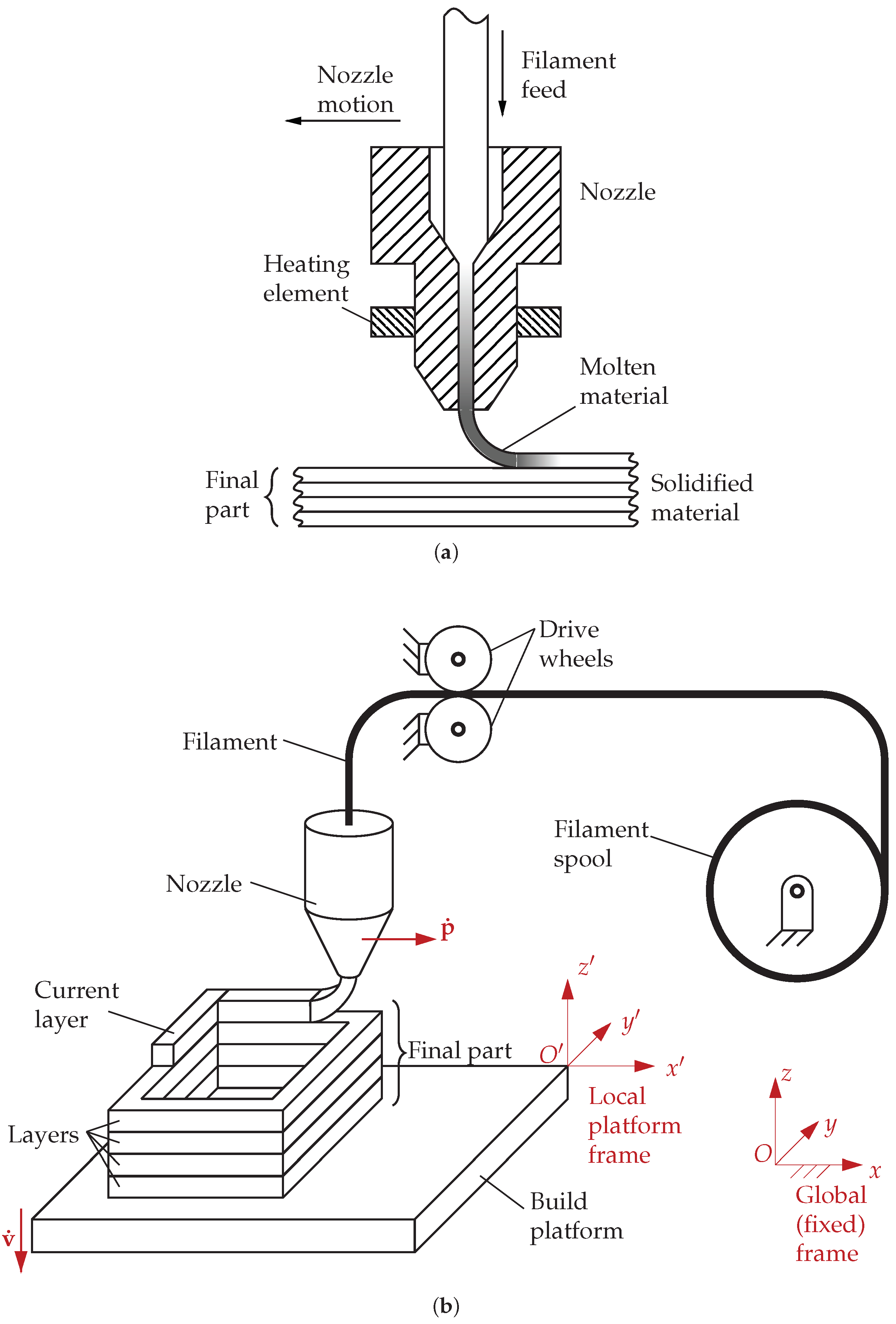
:1. Introduction
1.1. Architectures for 3D Printing
- (a)
- Cartesian mechanisms control the three components of the nozzle velocity (with respect to the build platform) along three coordinate axes independently; this greatly simplifies the kinematic analysis. Usually, the build platform has one DoF along one axis, while the nozzle has two DoFs along the other two axes. This is the most common architecture in desktop FDM printers [3,9,10,15,16,17,18,19,20,21].
- (b)
- Delta printers use the parallel kinematic architecture of the Delta robot, proposed by R. Clavel; in particular, the linear version of the Delta is used, where prismatic pairs actuate the mechanism [22]. With this architecture, the nozzle’s end-effector (EE) has only three translational DoFs, while the orientational DoFs are constrained. The main advantage is the fully parallel architecture, where the motors are fixed on the frame, which reduces the actuator torques. Moreover, the accuracy does not depend on the layer’s height above the build platform; thus, Delta printers are suited for printing parts that develop mostly along a vertical direction. On the other hand, their kinematics are more complex than those of Cartesian architectures; also, Delta printers have a smaller workspace with respect to the footprint.
- (c)
- SCARA printers use a robot arm with one translational and two rotational joints to move the nozzle [23]; the concept is derived from SCARA robots used in production lines [24]. While SCARA printers can provide a larger workspace than Delta printers, they are less rigid (and thus less accurate) due to their serial architecture.
- (d)
- Polar printers rotate the platform around a fixed axis, while the nozzle usually has two translational DoFs, along the vertical and the radial directions [25]. This design is cost-effective and leads to smaller footprints; however, the 3D printed part moves as the platform rotates, inducing vibrations that reduce the print accuracy.
- (e)
- Anthropomorphic architectures use a conventional serial arm, such as those of industrial robots used in production lines; unlike SCARA systems (type c), these generally have more than three DoFs. These mechanisms, thus, have greater freedom of motion and can realize more complex parts, but the issues related to the stiffness and the inertial effects of the serial architecture are even more pressing in this case e [26].
1.2. Kinematics for 3D Printers
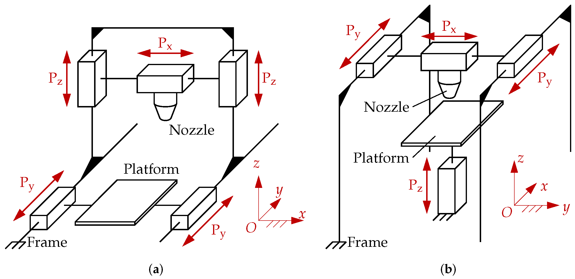
- (a.1)
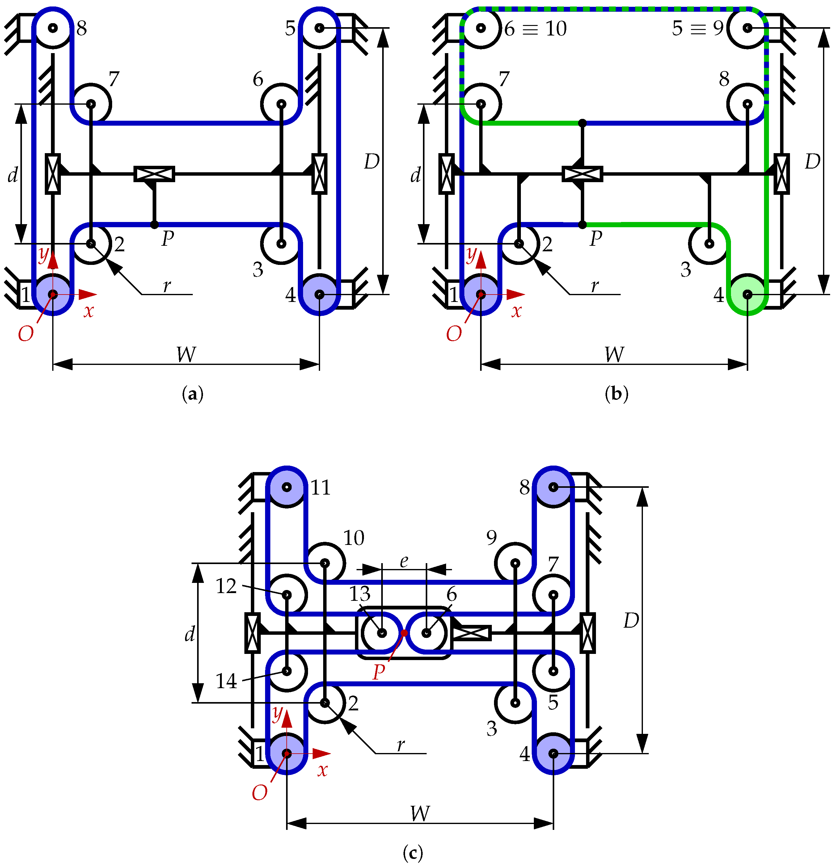
- XZ head printers (Figure 2a) have a frame with two vertical guides, along which a horizontal bar moves (along the z axis); on the said horizontal bar, the nozzle moves along the x axis. The motion along the y axis is applied to the platform instead. This is the most straightforward architecture, commonly employed in low-end printers for hobbyists. The main drawback is that increasing the print speed implies increasing the platform velocity (along the y axis), leading to rapid motions of the part being built, thus, inducing vibrations and lowering the accuracy. Moreover, the x-axis motor is attached to the horizontal bar, thus, increasing the moving mass.
- (a.2)
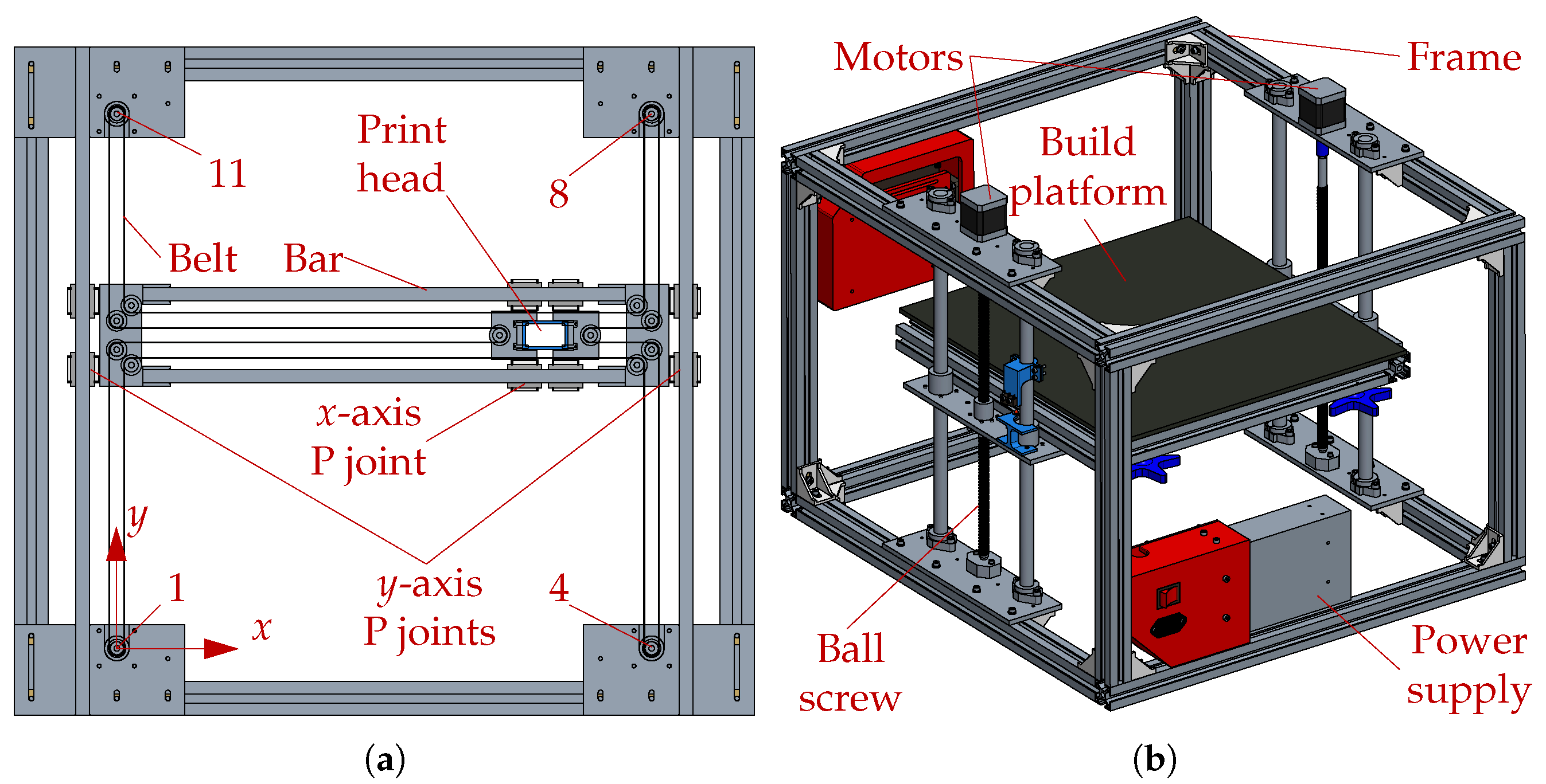
- In XY head printers (Figure 2b), the platform performs only motions along the z axis, which are much slower than those on the layer plane; thus, the accuracy is significantly increased. Furthermore, the workspace projection in the layer plane almost coincides with the footprint, which is, thus, smaller with respect to XZ head printers. This architecture is typical in high-end printers for professional use; while faster and more accurate, XY head printers are also more complex to design, and thus, more expensive.
- (a.2.i)
- A serial mechanism moves the nozzle along the y axis with motors fixed on the frame, while the motion along x is provided by a motor that is fixed on the bar. While this design is quite simple, the mass of the motor on the bar significantly increases the moving masses; thus, this option is seldom used [3,9,10].
- (a.2.ii)
- A stacked mechanism uses two stages: in each stage, the motor is fixed and causes a bar to move along guides. The stages are stacked on top of each other, with the second being rotated by 90 (along the z axis) with respect to the first. The nozzle is connected to both bars and can, thus, move on the x–y plane, its position being defined by the intersection of the two bars. While this approach reduces the moving masses, it significantly increases the printer size in the vertical direction and leads to a more complex design.
- (a.2.iii)
- A parallel mechanism usually has frame-fixed actuators; a parallel kinematic chain connects the motors to the nozzle. Often, a flexible element is used to transmit the movement; then, the bar and the lateral guides serve only to constrain the motion, which remains purely translational (on the horizontal plane).
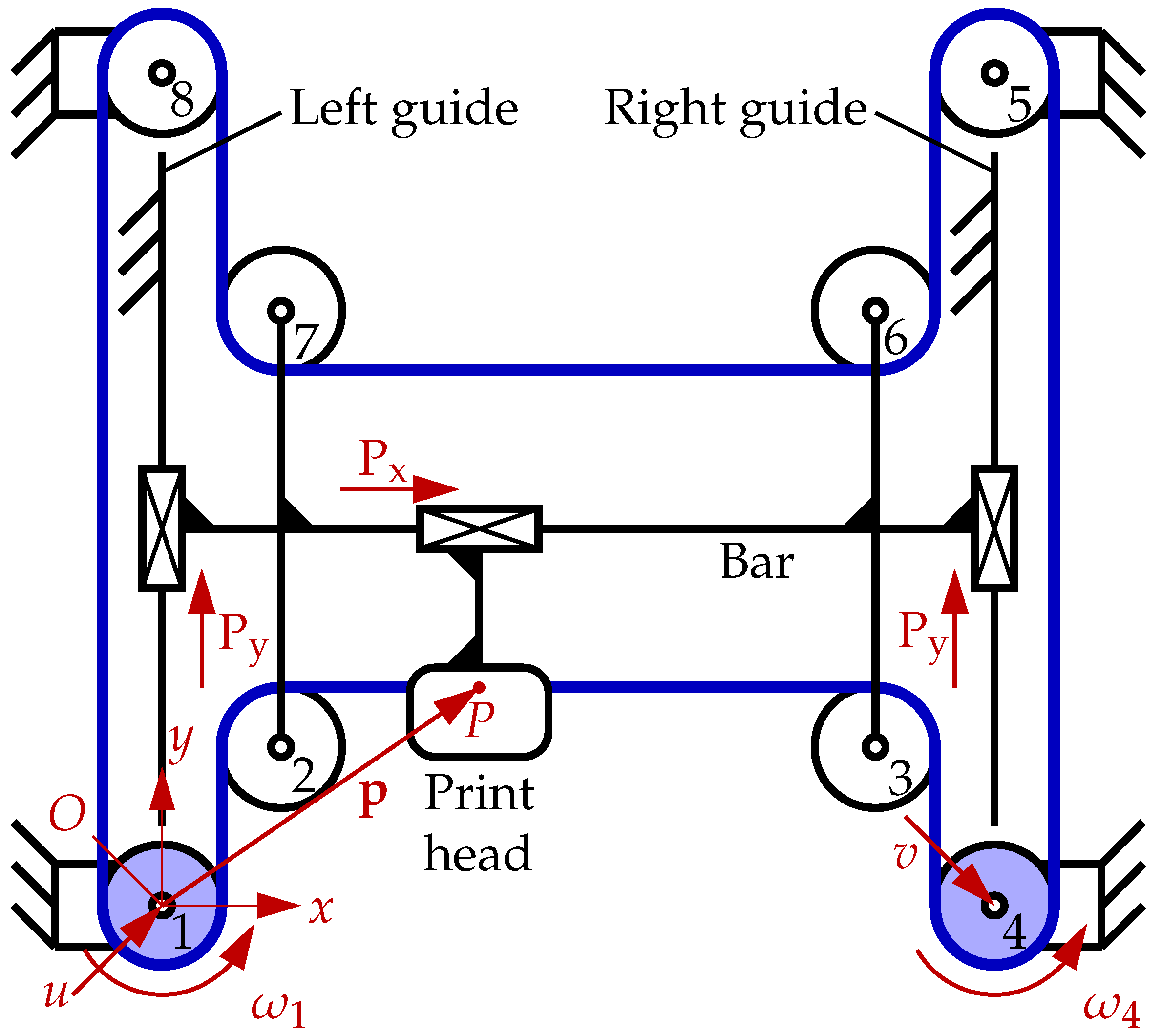
1.2.1. H-Bot
1.2.2. CoreXY
- Twist the overlapping segments (Figure 4) along the lengths so that they rotate around each other without crossing. This approach increases the belt stress and reduces the useful life; also, preventing the belt segments from touching each other is complex.
- Place the belts on parallel planes. This complicates the assembly and increases the printer volume; also, greater bending torques may be applied on the motor shaft.
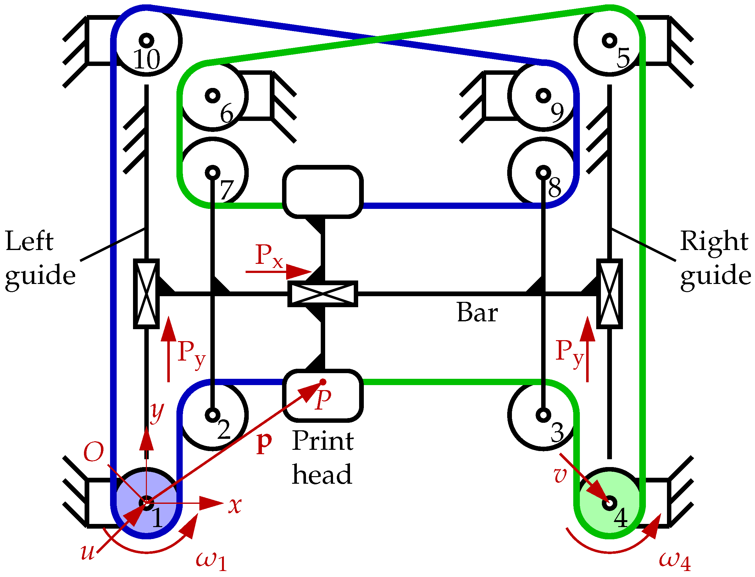
2. CoreH-Bot: Introduction and Kinematic Analysis
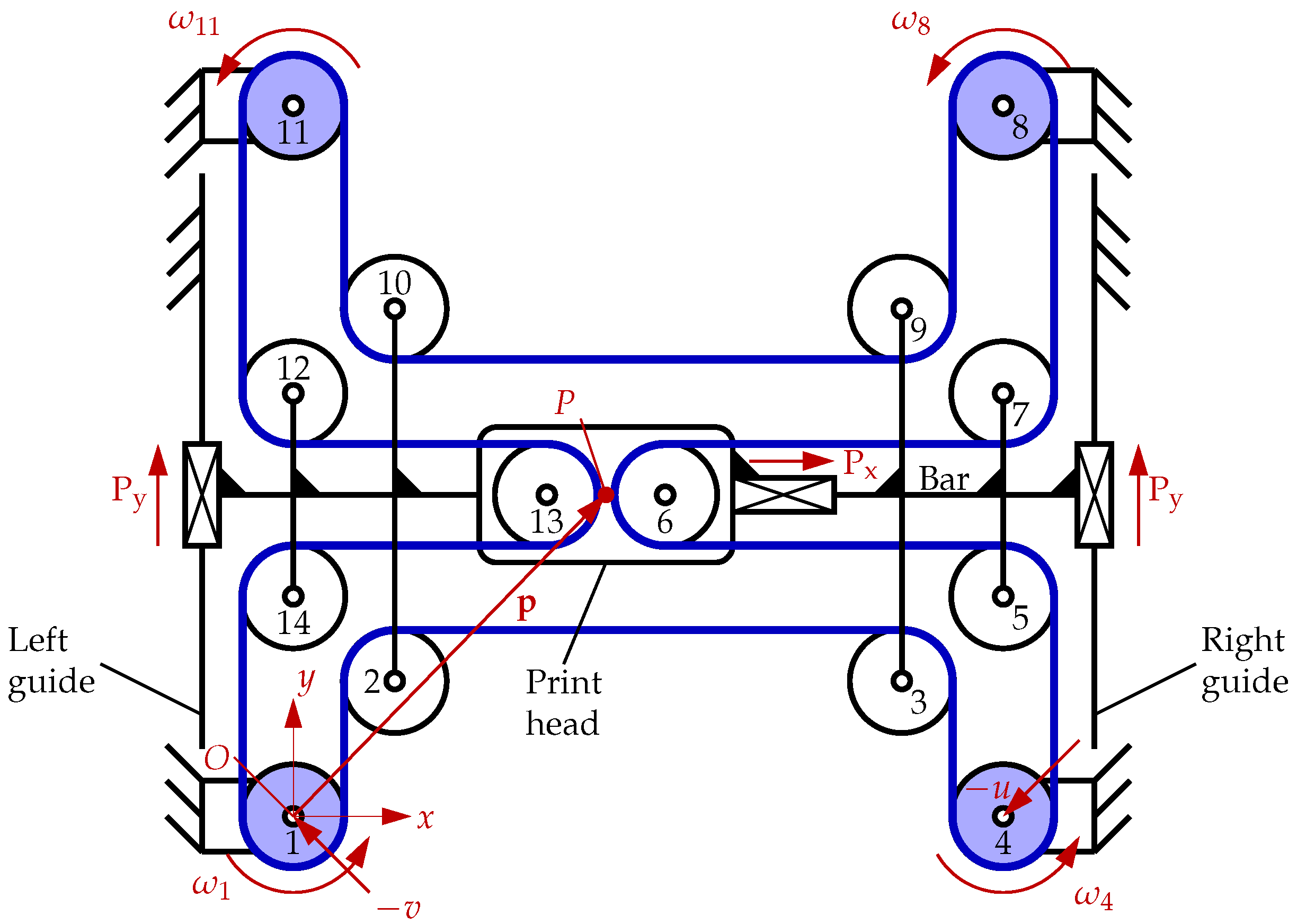
2.1. Introduction to the CoreH-Bot
2.2. Kinematic Analysis
- (I)
- all belt segments have constant orientation, along either the x- or the y-axis;
- (II)
- elastic deflections are disregarded and the belt length is the same under tension;
- (III)
- the belt is always in tension (that is, it does not become slack). This is achieved by a specific design (see Section 4), such that the tension is maintained during motion;
- (IV)
- the belt wraps on pulleys, and no slippage occurs between the belt and the pulleys;
- (V)
- the pulleys are connected by R joints to rigid blocks, either fixed or translating along one (or both) of the coordinate axes (with fixed orientation).
- Block-block constraints: these equations are written asThe first two equations of (4) correspond to fixing the frame position, while the remaining two correspond to the constraints introduced by the Py and Px joints, respectively. Notice that the two Py joints in Figure 5 are redundant, as they both introduce the same constraint (namely, that the bar can only translate along the y axis with respect to the frame); using two joints is only convenient for design purposes, to reduce the stresses on the components and increase the motion accuracy. Thus, only one Py joint is considered here without changing the DoFs of the mechanism.
- Pulley-block constraints: since the 14 pulleys are connected to the blocks by R joints, each removing two DoFs, 28 such equations are found, which can be written ascorresponding to the i-th pulley being connected to the j-th block.
- Belt-block constraints: no such equations are present, as the routing has a closed-loop configuration and the belt is not directly attached to any block.
- Belt-pulley constraints: the displacement of node is related to the rotation of the pulley that immediately precedes the corresponding cable segment and to the rotation of the next pulley (moving along the belt in a counterclockwise sense). For instance, the following equations can be written for node :The equations in (6) depend on the displacements of pulleys 1 and 2 along y since the belt segment at is parallel to the y axis; similar equations can be written for the segments parallel to the x axis (we refer the reader to [37] for details). A total of 28 equations can be written for the 14 belt segments.
3. Static and Dynamic Analysis
- (A)
- The belt is always taut and each belt segment is aligned either with the x or the y axis (see Section 2.2, conditions I and II). Thus, the forces transmitted by the belt segments to the pulleys are all directed along either the x or the y axis.
- (B)
- Elastic and frictional effects between the pulleys and the belt may be disregarded, and the force transmission is entirely due to the coupling between their profiles.
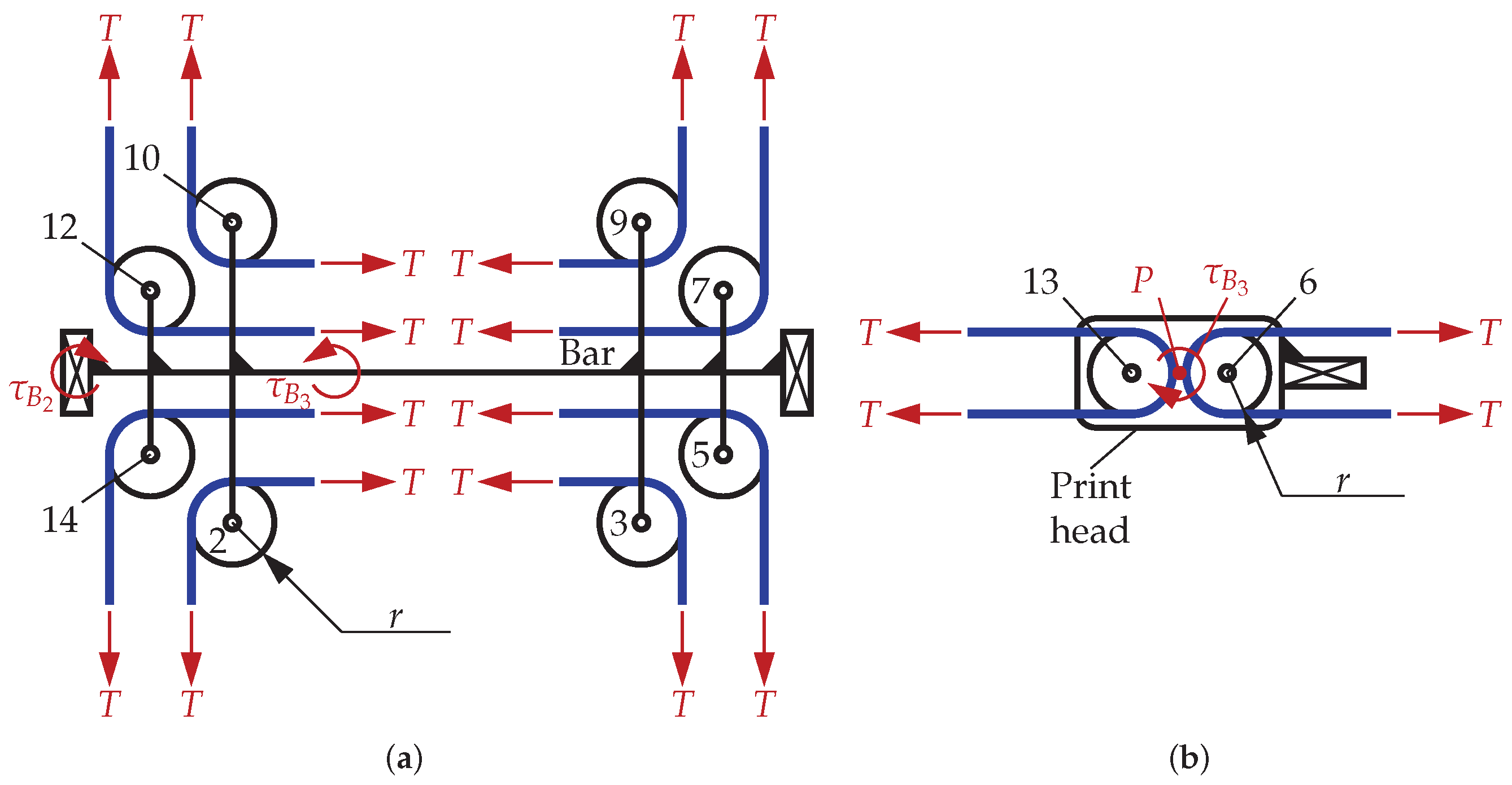
- (C)
- Inertial torques on the pulleys and frictional torques in the R joints (between the pulleys and the blocks on which they are mounted) can similarly be disregarded; thus, for an idle pulley, the forces in the two belt segments attached to it are always equal. For actuated pulleys, if the motor applies a torque, the tensions on the two segments are different so that the pulley is in equilibrium.
- (D)
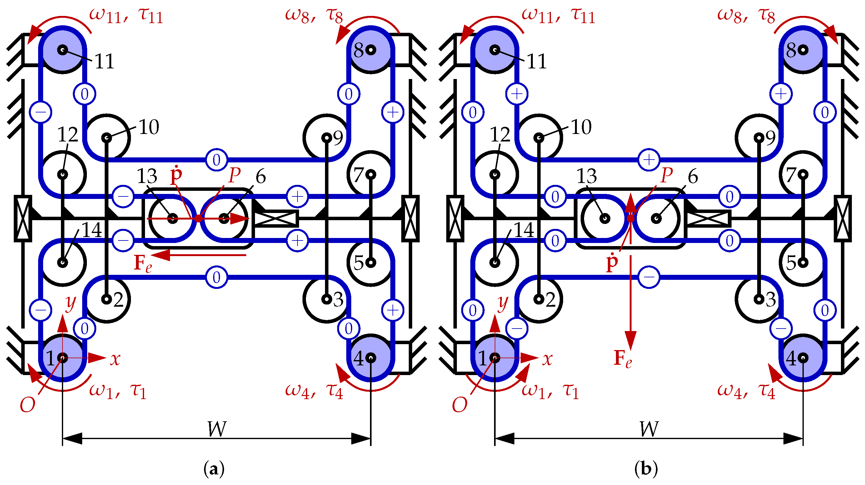
- Disregarding nonlinear force effects, the superposition principle applies; thus, we consider only two dynamic motions, namely, those along the x and the y axes, with the EE at a generic position. The results obtained will then be valid for a generic dynamic motion, and with the EE at any pose within the workspace, also considering that the Jacobian , as defined in Equation (1), is constant.
- (E)
- Under static conditions, the belt tension in each segment is constant and equal to T.
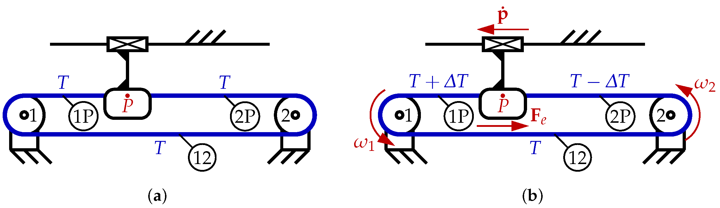
- (F)
- Under dynamic conditions, the belt tension changes with respect to the preload T. Some belt segments are under higher tension, as they are “pulled” by the closest actuated pulley, which rotates in a direction such that the corresponding displacements will be towards the said pulley. Other segments are instead “pushed” by an actuated pulley, such that the displacement is away from said pulley; thus, the tension in these segments will be lower. We assume that the changes in tension for the pulled and pushed segments are all constant and equal to and , respectively. Finally, some belt segments may be pushed and pulled at the same time; we assume that their tension does not change but remains equal to the preload T.As an example, in Figure 7, we show a simplified overconstrained routing, with one DoF and two actuated pulleys. In Figure 7a, the mechanism is in static equilibrium, and all belt segments have a tension equal to the preload T. In Figure 7b, on the other hand, a dynamic condition is shown, in which point P (of which the position defines the configuration of the routing) moves leftwards with velocity ; the pulleys rotate simultaneously at the same speed . A force is applied, opposite to : this could be due to inertial effects (if is not constant) or to friction. The tension in segment 1-P (from pulley 1 to P) increases by , the tension in segment 2-P decreases by , while in 1-2 the tension remains the same; we then have .
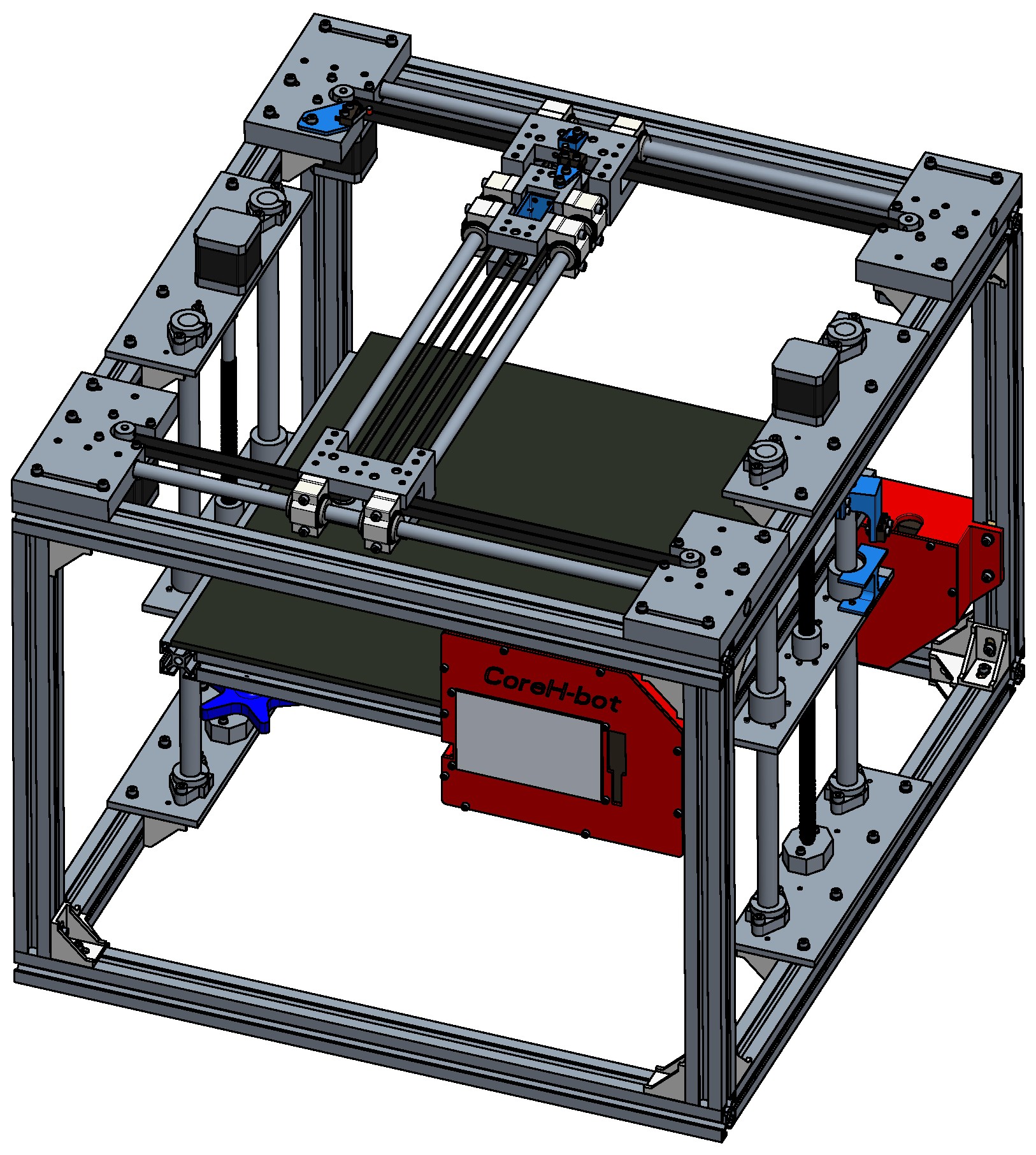
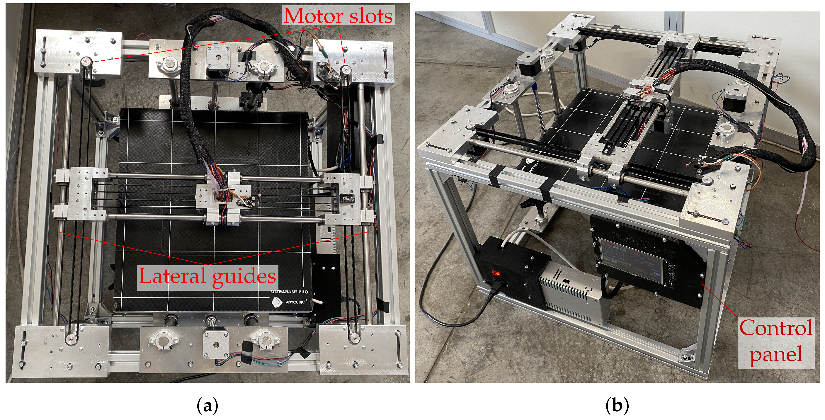
4. CoreH-Bot: Our Prototype
5. Conclusions and Future Work
6. Patents
Author Contributions
Funding
Acknowledgments
Conflicts of Interest
References
- Pham, D.T.; Gault, R.S. A comparison of rapid prototyping technologies. Int. J. Mach. Tools Manuf. 1998, 38, 1257–1287. [Google Scholar] [CrossRef]
- Gibson, I.; Rosen, D.W.; Stucker, B.; Khorasani, M. Additive Manufacturing Technologies; Springer: Berlin/Heidelberg, Germany, 2021. [Google Scholar] [CrossRef]
- Kodama, H. Automatic method for fabricating a three-dimensional plastic model with photo-hardening polymer. Rev. Sci. Instrum. 1981, 52, 1770–1773. [Google Scholar] [CrossRef]
- Hull, C.W. Apparatus for Production of Three-Dimensonal Objects by Stereolithography. United States Patent 4575330, 1986. Available online: https://patents.google.com/patent/US4575330A/en (accessed on 17 June 2022).
- Standard EN ISO/ASTM 52900:2021; Additive Manufacturing—General Principles—Fundamentals and Vocabulary. International Organization for Standardization: Geneva, Switzerland, 2021. Available online: https://www.iso.org/standard/74514.html (accessed on 17 June 2022).
- Wong, K.V.; Hernandez, A. A review of additive manufacturing. Int. Sch. Res. Not. 2012, 2012, 208760. [Google Scholar] [CrossRef] [Green Version]
- Scott, J.; Gupta, N.; Weber, C.; Newsome, S.; Wohlers, T.; Caffrey, T. Additive Manufacturing: Status and Opportunities; Technical report; Science and Technology Policy Institute: Washington DC, USA, 2012; Available online: https://www.researchgate.net/profile/Justin-Scott-4/publication/312153354_Additive_Manufacturing_Status_and_Opportunities/links/59e786db458515c3630f917b/Additive-Manufacturing-Status-and-Opportunities.pdf (accessed on 17 June 2022).
- Ngo, T.D.; Kashani, A.; Imbalzano, G.; Nguyen, K.T.Q.; Hui, D. Additive manufacturing (3D printing): A review of materials, methods, applications and challenges. Compos. Part B Eng. 2018, 143, 172–196. [Google Scholar] [CrossRef]
- Crump, S.S. Apparatus and Method for Creating Three-Dimensional Objects. United States Patent US5121329A, 9 June 1992. Available online: https://patents.google.com/patent/US5121329A/en (accessed on 17 June 2022).
- Shah, J.; Snider, B.; Clarke, T.; Kozutsky, S.; Lacki, M.; Hosseini, A. Large-scale 3D printers for additive manufacturing: Design considerations and challenges. Int. J. Adv. Manuf. Technol. 2019, 104, 3679–3693. [Google Scholar] [CrossRef]
- Campana, G.; Mele, M.; Ciotti, M.; Rocchi, A. Environmental impacts of self-replicating three-dimensional printers. Sustain. Mater. Technol. 2021, 30, e00335. [Google Scholar] [CrossRef]
- Ciotti, M.; Campana, G.; Mele, M. A review of the accuracy of thermoplastic polymeric parts fabricated by additive manufacturing. Rapid Prototyp. J. 2021, 28, 358–389. [Google Scholar] [CrossRef]
- Ligon, S.C.; Liska, R.; Stampfl, J.; Gurr, M.; Mülhaupt, R. Polymers for 3D printing and customized additive manufacturing. Chem. Rev. 2017, 117, 10212–10290. [Google Scholar] [CrossRef] [Green Version]
- Turner, B.N.; Strong, R.; Gold, S.A. A review of melt extrusion additive manufacturing processes: I. Process design and modeling. Rapid Prototyp. J. 2014, 20, 192–204. [Google Scholar] [CrossRef]
- Go, J.; Hart, A.J. Fast desktop-scale extrusion additive manufacturing. Addit. Manuf. 2017, 18, 276–284. [Google Scholar] [CrossRef] [Green Version]
- Vasquez, J.; Twigg-Smith, H.; O’Leary, J.T.; Peek, N. Jubilee: An extensible machine for multi-tool fabrication. In Proceedings of the 2020 CHI Conference on Human Factors in Computing Systems, Honolulu, HI, USA, 25–30 April 2020; Association for Computing Machinery: Honolulu, HI, USA, 2020. [Google Scholar] [CrossRef]
- Edoimioya, N.; Ramani, K.S.; Okwudire, C.E. Software compensation of undesirable racking motion of H-frame 3D printers using filtered B-splines. Addit. Manuf. 2021, 47, 102290. [Google Scholar] [CrossRef]
- Weikert, S.; Ratnaweera, R.; Zirn, O.; Wegener, K. Modeling and measurement of H-Bot kinematic systems. In Proceedings of the 26th Annual Meeting American Society for Precision Engineering, Denver, CO, USA, 18 November 2011; ASPE: Denver, CO, USA, 2011. Available online: https://www.iwf.mavt.ethz.ch/ConfiguratorJM/publications/MODELING_A_132687166151936/3314_mod.pdf (accessed on 17 June 2022).
- Comb, J.W.; Swanson, W.J.; Crotty, J.L. Gantry assembly for Use in Additive Manufacturing System. United States Patent US20130078073A1, 28 March 2013. Available online: https://patents.google.com/patent/US20130078073A1/en (accessed on 17 June 2022).
- Peek, N.; Moyer, I. Popfab: A case for portable digital fabrication. In Proceedings of the 11th International Conference on Tangible Embedded, and Embodied Interaction, Yokohama, Japan, 20–23 March 2017; Association for Computing Machinery: Yokohama, Japan, 2017; pp. 325–329. [Google Scholar] [CrossRef]
- Avdeev, A.R.; Shvets, A.A.; Torubarov, I.S. Investigation of kinematics of 3D printer print head moving systems. In Proceedings of the 5th International Conference on Industrial Engineering (ICIE 2019), Sochi, Russia, 25–29 March 2019; Lect. Notes Mechanical Engineering; Springer: Berlin/Heidelberg, Germany, 2019; pp. 461–471. [Google Scholar] [CrossRef]
- Clavel, R. Device for the Movement and Positioning of an Element in Space. United States Patent US4976582A, 11 December 1990. Available online: https://patents.google.com/patent/US4976582A/en (accessed on 17 June 2022).
- Záda, V.; Belda, K. Structure design and solution of kinematics of robot manipulator for 3D concrete printing. IEEE Trans. Autom. Sci. Eng. 2022. [Google Scholar] [CrossRef]
- Furuya, N.; Makino, H. Research and development of selective compliance assembly robot arm (1st report)—Characteristics of the system. J. Jpn. Soc. Precis. Eng. 1980, 46, 1525–1531. [Google Scholar] [CrossRef]
- Zhao, D.; Li, T.; Shen, B.; Jiang, Y.; Guo, W.; Gao, F. A multi-DOF rotary 3D printer: Machine design, performance analysis and process planning of curved layer fused deposition modeling (CLFDM). Rapid Prototyp. J. 2020, 26, 1079–1093. [Google Scholar] [CrossRef]
- Urhal, P.; Weightman, A.; Diver, C.; Bartolo, P. Robot assisted additive manufacturing: A review. Robot. Comput. Integr. Manuf. 2019, 59, 335–345. [Google Scholar] [CrossRef]
- Vu, D.S.; Foucault, S.; Gosselin, C.; Kövecses, J. Design of a locomotion interface for gait simulation based on belt-driven parallel mechanisms. In Proceedings of the 2015 IEEE International Conference on Robotics and Automation (ICRA), Seattle, WA, USA, 26–30 May 2015; IEEE: Seattle, WA, USA, 2015; pp. 1581–1586. [Google Scholar] [CrossRef]
- Vu, D.S.; Kövecses, J.; Gosselin, C. Trajectory planning and control of a belt-driven locomotion interface for flat terrain walking and stair climbing. In Proceedings of the 2017 IEEE World Haptics Conference (WHC), Munich, Germany, 6–9 June 2017; IEEE: Fürstenfeldbruck, Germany, 2017; pp. 189–194. [Google Scholar] [CrossRef]
- Gosselin, C.; Laliberté, T. On the development of a walking rehabilitation device with a large workspace. In Proceedings of the IEEE 2011 ICORR, Zurich, Switzerland, 29 June–1 July 2011; IEEE: Zurich, Switzerland, 2011. [Google Scholar] [CrossRef]
- Gosselin, C.; Laliberté, T.; Mayer-St-Onge, B.; Foucault, S.; Lecours, A.; Duchaine, V.; Paradis, N.; Gao, D.; Menassa, R. A friendly beast of burden—A human-assistive robot for handling large payloads. IEEE Robot. Autom. Mag. 2013, 20, 139–147. [Google Scholar] [CrossRef]
- Forgó, Z.; Szilágyi, A. Dynamic modeling of new modular manipulators. In Proceedings of the 47st International Symposium on Robotics, Munich, Germany, 21–22 June 2016; IEEE: Munich, Germany, 2016; pp. 515–520. Available online: https://ieeexplore.ieee.org/abstract/document/7559162 (accessed on 17 June 2022).
- Forgó, Z.; Tolvaly-Roşca, F. Analytical and numerical model of low DOF manipulators. Proc. Technol. 2015, 19, 40–47. [Google Scholar] [CrossRef] [Green Version]
- Zhu, J.; Li, B.; Mu, H.; Li, Q. Kinematic analysis of a flexible planar 2-DOF parallel manipulator. In Lecture Notes in Computer Science, Proceedings of the International Conference on Intelligent Robotics and Applications (ICIRA 2019), Shenyang, China, 8–11 August 2019; Springer: Shenyang, China, 2019; Volume 11744, pp. 696–706. [Google Scholar] [CrossRef]
- Perneder, R.; Osborne, I. Handbook Timing Belts—Principles, Calculations, Applications; Springer: Berlin/Heidelberg, Germany, 2012. [Google Scholar] [CrossRef]
- Laliberté, T.; Gosselin, C.; Gao, D. Closed-loop transmission routings for Cartesian SCARA-type manipulators. In Proceedings of the ASME 2010 IDETC/CIE, Montreal, QC, Canada, 15–18 August 2010; ASME: Montreal, QC, Canada, 2010; Volume 2, pp. 281–290. [Google Scholar] [CrossRef]
- Behzadipour, S. Kinematics and dynamics of a self-stressed Cartesian cable-driven mechanism. J. Mech. Des. 2009, 131, 061005. [Google Scholar] [CrossRef]
- Hong, D.W.; Cipra, R.J. A method for representing the configuration and analyzing the motion of complex cable-pulley systems. J. Mech. Des. 2003, 125, 332–341. [Google Scholar] [CrossRef]
- Webster, D.C. Recording Mechanism. United States Patent US2675291A, 13 April 1954. Available online: https://patents.google.com/patent/US2675291A/en (accessed on 17 June 2022).
- Sollmann, K.S.; Jouaneh, M.K.; Lavender, D. Dynamic modeling of a two-axis, parallel, H-frame-type XY positioning system. IEEE/ASME Trans. Mechatron. 2009, 15, 280–290. [Google Scholar] [CrossRef]
- Rice, Q. X-Y Workhead Positioning Device. Great Britain patent. 1994. Available online: https://patents.google.com/patent/GB2274719A/en (accessed on 17 June 2022).
- Linhart, C.H. X-ray Apparatus Comprising a Film Cassette Which Is Displaceable in a Carrage. United States Patent US4961213A, 2 October 1990. Available online: https://patents.google.com/patent/US4961213A/en (accessed on 17 June 2022).
- Kerschner, R.K. Differential Motor Drive for an XY Stage. United States Patent US6070480A, 2000. Available online: https://patents.google.com/patent/US6070480A/en (accessed on 17 June 2022).
- Fustinoni, E. Apparatus for Laser Cutting and/or Marking. United States Patent US20070221621A1, 2007. Available online: https://patents.google.com/patent/US20070221621A1/en (accessed on 17 June 2022).
- Etcheparre, J.; Etcheparre, B. Device for Driving and Displacing a Beam Resting Upon Guide Rails, and One or More Carriages Attached to the Beam. United States Patent US4315437A, 1982. Available online: https://patents.google.com/patent/US4315437A/en (accessed on 17 June 2022).
- Budzyn, B.L. Chain Drive System for Mobile Loading Platform or for Two- or Three-Dimensional Indexing. United States Patent US3529481A, 1970. Available online: https://patents.google.com/patent/US3529481A/en (accessed on 17 June 2022).
- Forgó, Z. Mathematical modelling of 4 DOF gantry type parallel manipulator. In Proceedings of the 41st International Symposium on Robotics and 6th German Conference on Robotics, Munich, Germany, 7–9 June 2010; IEEE: Munich, Germany, 2010; pp. 1206–1211. Available online: https://ieeexplore.ieee.org/abstract/document/5756939 (accessed on 17 June 2022).
- Harada, T. Novel Schönflies motion parallel robot driven by differential mechanism. Int. J. Mech. Eng. Robot. Res. 2020, 9, 106–110. [Google Scholar] [CrossRef]
- Chen, Y.; Squires, A.; Seifabadi, R.; Xu, S.; Agarwal, H.K.; Bernardo, M.; Pinto, P.A.; Choyke, P.; Wood, B.; Tse, Z.T.H. Robotic system for MRI-guided focal laser ablation in the prostate. IEEE/ASME Trans. Mechatron. 2017, 22, 107–114. [Google Scholar] [CrossRef] [PubMed]
- Mottola, G.; Gosselin, C.; Carricato, M. Effect of actuation errors on a purely-translational spatial cable-driven parallel robot. In Proceedings of the 9th IEEE CYBER, Bengkulu, Indonesia, 22–23 September 2021; IEEE: Suzhou, China, 2019; pp. 701–707. [Google Scholar] [CrossRef]
- Waldron, K.J.; Hunt, K.H. Series-parallel dualities in actively coordinated mechanisms. Int. J. Robot. Res. 1991, 10, 473–480. [Google Scholar] [CrossRef]
- Zi, B.; Wang, N.; Qian, S.; Bao, K. Design, stiffness analysis and experimental study of a cable-driven parallel 3D printer. Mech. Mach. Theory 2019, 132, 207–222. [Google Scholar] [CrossRef]


| Segment | Length | Segment | Length | Segment | Length |
|---|---|---|---|---|---|
| 1–2 | 6–7 | 11–12 | |||
| 2–2 | 7–7 | 12–12 | |||
| 2–3 | 7–8 | 12–13 | |||
| 3–3 | 8–8 | 13–13 | |||
| 3–4 | 8–9 | 13–14 | |||
| 4–4 | 9–9 | 14–14 | |||
| 4–5 | 9–10 | 14–1 | |||
| 5–5 | 10–10 | 1–1 | |||
| 5–6 | 10–11 | ||||
| 6–6 | 11–11 |
| Definition | Value |
|---|---|
| Width W (equal to depth D) | 470 mm |
| Pulley radius r at pitch circle | 6.35 mm |
| Distance d (pulleys on bar) | 52.4 mm |
| Distance e (pulleys on head) | 80 mm |
| Heated bed (print area size) | mm |
| Motion range (along z axis) | 335 mm |
| Ball screw diameter and pitch | M12 × 4 |
| Diameter of x–y plane bars | 12 mm |
| Total length of belt loop | 3600 mm |
| GT2 belt pitch and height | mm |
| Frame profile (cross section) | mm |
Publisher’s Note: MDPI stays neutral with regard to jurisdictional claims in published maps and institutional affiliations. |
© 2022 by the authors. Licensee MDPI, Basel, Switzerland. This article is an open access article distributed under the terms and conditions of the Creative Commons Attribution (CC BY) license (https://creativecommons.org/licenses/by/4.0/).
Share and Cite
Idà, E.; Nanetti, F.; Mottola, G. An Alternative Parallel Mechanism for Horizontal Positioning of a Nozzle in an FDM 3D Printer. Machines 2022, 10, 542. https://doi.org/10.3390/machines10070542
Idà E, Nanetti F, Mottola G. An Alternative Parallel Mechanism for Horizontal Positioning of a Nozzle in an FDM 3D Printer. Machines. 2022; 10(7):542. https://doi.org/10.3390/machines10070542
Chicago/Turabian StyleIdà, Edoardo, Federico Nanetti, and Giovanni Mottola. 2022. "An Alternative Parallel Mechanism for Horizontal Positioning of a Nozzle in an FDM 3D Printer" Machines 10, no. 7: 542. https://doi.org/10.3390/machines10070542