Article

Velocity Estimation and Cost Map Generation for Dynamic Obstacle Avoidance of ROS Based AMR

1
Graduate Institute of Automation Technology, National Taipei University of Technology, Taipei 10608, Taiwan
2
Smart Automation Unit, TECO Electric & Machinery Co., Ltd., 10F, No. 3-1, Park St., Nan-Kang, Taipei 11503, Taiwan
3
Department of Electrical Engineering, National Yunlin University of Science and Technology, Douliou, Yunlin 64002, Taiwan
*
Author to whom correspondence should be addressed.
Machines 2022, 10(7), 501; https://doi.org/10.3390/machines10070501
Submission received: 31 May 2022 / Revised: 16 June 2022 / Accepted: 17 June 2022 / Published: 22 June 2022
(This article belongs to the Special Issue Recent Applications of Assistive Robots)

Abstract

:
In the past few years, due to the growth of the open-source community and the popularity of perceptual computing resources, the ROS (Robotic Operating System)Ecosystem has been widely shared and used in academia, industrial applications, and service fields. With the advantages of reusability of algorithms and system modularity, service robot applications are flourishing via the released ROS navigation framework. In the ROS navigation framework, the grid cost maps are majorly designed for path planning and obstacle avoidance with range sensors. However, the robot will often collide with dynamic obstacles since the velocity information is not considered within the navigation framework in time. This study aims to improve the feasibility of high-speed dynamic obstacle avoidance for an ROS-based mobile robot. In order to enable the robot to detect and estimate dynamic obstacles from a first-person perspective, vision tracking and a laser ranger with an Extend Kalman Filter (EKF) have been applied. In addition, an innovative velocity obstacle layer with truncated distance is implemented for the path planner to analyze the performances between the simulated and actual avoidance behavior. Finally, via the velocity obstacle layer, as the robot faces the high-speed obstacle, safe navigation can be achieved.

1. Introduction

Based on the rapid development of intelligent sensing technology and the high resource sharing of the Robot Operation System (ROS) robot community, service robots have gradually shifted into commercial applications from the academic field in daily life, such as food delivery, logistics, and security monitoring. The key design of service robot development includes stable autonomous navigation, as well as safety and obstacle avoidance. To prevent a collision during service operations, the robot needs to immediately consider static and dynamic obstacles, for example, passing through items of furniture and persons who are walking by.
Nowadays, the ROS framework is widely used for autonomous mobile robot (AMR) development. The “move base” library of the ROS framework was specifically implemented for autonomous navigation with obstacle avoidance based on the “grid cost map”. The grid cost map may consist of different layers, such as the static map layer and the sensor’s information layer, which are implemented for global and local path planning. However, when the mobile robot encounters a dynamic obstacle, the robot will often collide with the moving obstacle due to the mobile robot’s inability to predict the dynamic information of the moving obstacle, such as the direction, the velocity, and the collision region.
In the past, Velocity Obstacle (VO) studies have demonstrated good results in obstacle avoidance in the gaming field, assuming that all the velocities of dynamic obstacles are known in advance. However, it is not easy to estimate the velocity of obstacles nearby the robot itself in first-person view. In this study, we try to enhance the robot’s observation of the dynamic obstacles. Firstly, the segmentation of spatial objects, the 2D laser ranger, and the 3D vision camera are applied with the Extended Kalman Filter (EKF) to estimate the velocity of each dynamic obstacle. In addition, we propose the innovative concept of generating a new velocity obstacle layer of the grid cost map for the ROS navigation stack, which improves the navigation utility by combining the static characteristics of the obstacles on the original grid cost map with the new velocity obstacle layer.
The main contribution of this research is to improve the obstacle avoidance behavior of the mobile robot when encountering high-speed moving obstacles in the process of navigation with the innovative new speed obstacle layer and cut-off distance calculation algorithm design. In addition, we put forward an optimization of the ROS navigation framework, applying innovative results to the Cost Map and DWA Path planner. The results are imported into the mobile robot and run in the field. The experimental result shows the comparison of navigation behavior with the default ROS utility that has been proven to be more stable and flexible in high-speed obstacle avoidance in terms of the AMR pre-scheduling a safer path. Finally, the article organization is as follows: Section 2 reviews the previous related works of this study, Section 3 focuses on the implementation of obstacle identification and estimation, Section 4 optimizes and implements VO in the ROS cost map framework, Section 5 presents the simulation and actual experimental results, and Section 6 presents the discussion and conclusion.

2. Related Works

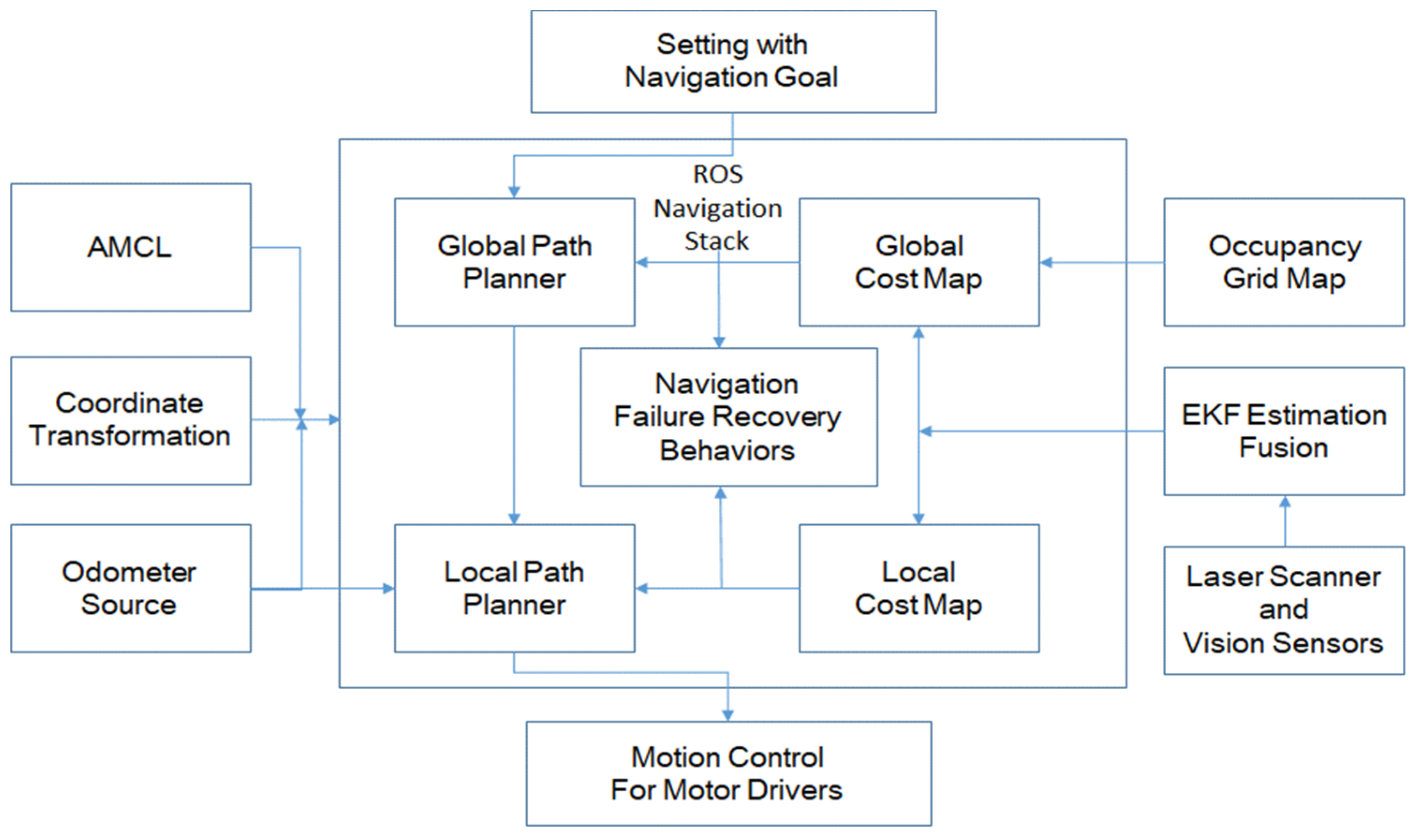
2.1. Navigation Framework via ROS

In the past few years, robot navigation technology has grown rapidly in the development and demonstration of the ROS community [1]. Figure 1 shows the most common navigation framework for autonomous mobile robots [2]. The topic “/maps” is published from the Map-Server of the ROS package, which is key information obtained via simultaneous localization and mapping (SLAM) execution. Today, SLAM algorithms mainly use laser ranger sensors and vision cameras. The laser ranger based includes Gmapping SLAM [3], Hector SLAM [4], Cartographer SLAM [5], etc., and the popular vision-based SLAM such as the ORB-SLAM [6].
For robot-self localization, the positioning information of the robot can be referenced via the odometer. The odometer is accumulated from the encoder to count the feedback of the wheel rotation. The slippage of the robot wheel and the ground will cause the accumulated error; the Adaptive Monte Carlo Localization (AMCL) [7] is typically a robot-self-localization algorithm using a laser ranger and odometer. The odometer provides a dead reckoning estimation for each particle of AMCL as the robot’s possible pose. By applying the laser ranger sensing, the AMCL will statistically converge the robot’s pose based on the static map from the Map-Server. Since the improvement in computing performance has made the ORB-SLAM visual positioning algorithm the mainstay of recent research, in addition to Bluetooth/UWB/GPS application development [8,9], applicable positioning technology for robot-self localization has steadily gained acceptance over the past decade. In addition, the robot can detect obstacles, and it can use different sensors, such as monocular cameras, stereo cameras, RGB-D cameras, a laser ranger, a millimeter-wave radar, and ultrasound, to perform obstacle detection, as the sensor sources of Figure 1.

2.2. Cost Map with Multi-Layer

Cost map plays a very important role in the ROS navigation architecture, which is obtained by sensors and converts the map information into a form that is easy to interpret by the path planner. When the robot is in operation, different cost maps are used to express the perception status obtained by the respective sensors so that it can avoid all obstacles when navigating or exploring tasks. It is like a human being organizing the information obtained by the eyes, ears, and touch as to whether it is passable or not. The cost map in the ROS navigation architecture usually may have more than one layer, as shown in Figure 2. It combines a static layer, an obstacle layer, an expansion layer, and a master control layer. The cost map is unified by the main control layer from different sensor layers for navigation missions and is represented in the form of a grid. The value of each grid ranges from 0 to 254, with higher values indicating a higher risk of entering the area, which implies that the grid is occupied by an obstacle.
When the static layer receives spatial information, it updates and calculates the boundary area covering the entire map during the initialization. The boundary area usually does not change in the subsequent static layer because the static layer is generated by the SLAM static map. As the basis of the global cost map, the static layer will be the first layer to update the cost values to the main cost map and copy all the values to the main cost map. The obstacle layer will be updated periodically, collecting data from sensors, such as a 2D laser ranger and an RGB-D camera. The region between the sensor and obstacle is free, the value is null for no occupation, and the region of the sensor reading value is updated with a high value for occupied. The purpose of the expansion layer is to give a buffer zone to prevent the robot from colliding too close to obstacles, and the area where the robot will collide is called the fatal zone. The highest cost value 254 is given in this area, and the surrounding cost is directly dependent on an exponential decay function such as in (1), this area is the aforementioned buffer zone. Update bounds will change with the increase in the inflated area to ensure that all inflated layers are updated to the main cost map.
  C = e x p α · d o b s r i n s · V t h e a l
where
C: cost values in a grid cell,
α: scale factor of decay rate,
dobs: distance from obstacle,
rins: robot’s inscribed radius,
Vtheal: lethal cost values (Default: 254).
In addition to the classic Static Layer, Obstacle Layer, Inflation Layer, and Master Layer on the cost map structure in the ROS framework, many robotics experts have also developed special layers for different scenarios. For example, the spatial-temporal voxel layer has super-high-performance computing power when converting 3D obstacles into voxel-based cost maps. The navigation layer (Nav Layer) uses a depth camera to determine if there are dangerous areas in 3D space with rugged ground or stairs that look like cliffs and mark them with a 2D cost map, or it can set certain prohibition layers that are not allowed to be entered by a robot [10].

2.3. Global Path Planner

Based on robot-self localization, the global planner is a pre-planning method that depends on the analysis of a known global cost map. The global path planning algorithm will find a path avoiding static obstacles through this global cost map so that the robot can follow a path from the starting point to the goal point. At present, common global path planners include the A* algorithm [11], Dijkstra’s algorithm [12], and Rapidly Exploring Random Trees (RRTs) [13]. Under the ROS architecture, Dijkstra’s algorithm is applied for the default algorithm. Although the search time of the algorithm will be slower than the random sampling method, compared to the time taken from the robot navigation, it is more beneficial to spend a few milliseconds to find the shortest path than if the robot walks one meter longer. Dijkstra’s algorithm will start from the original point to search for the neighboring grids and then traverse the grids near the searched grids until the goal point is found. This algorithm is classified as a breadth-first algorithm, which can find the shortest path because it has a wider search for the map.

2.4. Local Path Planner

The main purpose of local path planning is to calculate the speed command to control the robot to navigate according to the path generated by the global path planner. The area of the local path planner usually sets a rectangle region with the center as the robot’s position. In this rectangle region, the local path planner will be responsible for the safety and calculating the optimal speed command. If the path generated by the global path planner is occupied by obstacles, the local path planner will find a new path connecting the original global path as much as possible. However, if the global path is not passable, it will send a message to the global path planning algorithm to recalculate a new path. If the obstacle makes the robot unable to move, then the recovery behavior (Recovery Behavior) mechanism will be activated to clear the surrounding cost map to confirm whether it is impassable.
The local path planning algorithm uses the Dynamic Window Approach method (DWA) [14], which combines the kinematic properties of the robot by sampling multiple sets of linear and angular velocities in the velocity space (𝜈, 𝜔) and conditioning the velocity space. It is expected that for the trajectory of the robot in a short time interval under the sampling speed, the sampled speed must meet the three objectives: (1) avoid obstacles that may collide; (2) the speed can be achieved within the time interval; (3) the target point can be reached quickly. DWA can easily and effectively avoid static obstacles, but the obstacles with speed information may collide. To solve this problem, it is necessary to improve the simulation time during sampling time to avoid the obstacles, as shown in Figure 3. Because DWA only includes the period of obstacle information when conducting velocity sampling and does not consider the moving speeds and direction of distant obstacles, the general solution is to increase the simulation time of obstacle sampling.
However, reference [15] mentions that all simulated trajectories are simple arcs, and if the simulation time is increased, it will produce long curves that are not very flexible in the simulation area so that the robot cannot perform optimal path navigation, and on the contrary, a simulation time that is too low will lead to performance limitations.

2.5. Velocity Obstacle

The existing motion planning method has been well established and has good execution ability in a dynamic or a static environment. The velocity obstacle algorithm was first used in the mutual obstacle avoidance of multiple robots [16]. The premise is that each machine can transmit the robot radius, speed, and position information to each other and then calculate the safe collision area.
VO also has many extensions. For example, it is used to solve the problem of jitter when two robots are approaching, or the vertex is too close to the origin of the velocity space so that the robot cannot move. This problem can be solved by truncating the speed obstacle area such as the Reciprocal Velocity Obstacles (RVO) [17], which is proposed for collision avoidance between the robots, and the well-known Particle Swarm Optimization (PSO) could be used to choose the best path for the robot maneuver to avoid colliding with other robots and enable it to reach its goal faster [18]. ORCA is an extension of RVO and is widely used in the navigation function of computer games. When large-scale players walk each other [19,20], the paper mentioned that it is difficult to avoid high-speed moving obstacles with existing motion planning methods. For social robot navigation in a complex crowded environment consideration, the robot can safely navigate in a crowd only if it can predict the next action of the humans; however, this task becomes difficult because of the unpredictable human behavior. Some researchers combine the VO concept of Danger-Zone [21] with an artificial reinforcement learning method to consider all possible actions that humans can take at a given time.

3. Obstacle Detection and Estimation

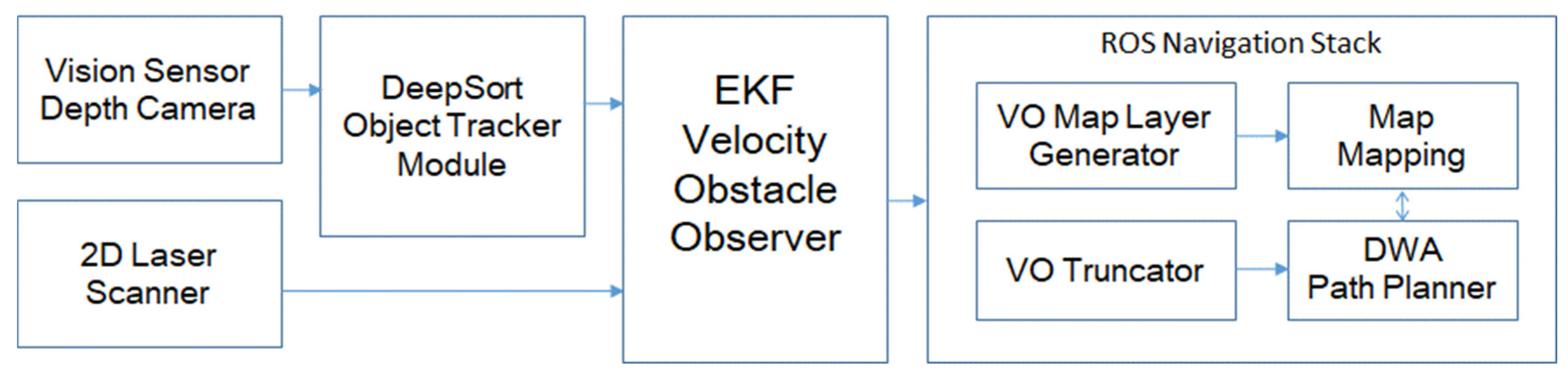
3.1. System Method Workflow

The architecture of the system software design is based on ROS communication and can be broken down into Drivers Layer, Control Core Layer, and Application Layer, as shown in Figure 4. The purpose of this research is to develop an ROS-based robot that can automatically detect high-speed moving obstacles and generate them in a cost map for obstacle avoidance during navigation. The system utilizes 2D laser scanning and a vision depth camera to detect high-speed moving obstacles. Image processing can enhance the robustness of obstacle detection on a two-dimensional plane. Through the DeepSORT object tracker module, the moving object can be locked, and information from the laser can be integrated and transmitted to the EFK velocity observer to generate the estimated velocity obstacle. A new VO cost layer can be generated in the original cost map by using the map layer generator. Via the VO truncator and the DWA path planner, we will improve the behavior of obstacle avoidance, as well as avoid collisions.

3.2. Tracking of Image Objects

The DeepSORT algorithm [22,23] is an extension of the Simple Online and Real-time Tracking (SORT) method. Based on a known trained model, it compares real-time images and generates a continuous moving frame called ROI (Region of Interest). Through pre-image processing, the robot can identify fast-moving crowds during the movement. Based on the Tracking-by-Detection strategy, it can effectively identify the space environment and moving obstacles and use the results of target detection to track obstacles.
Though DeepSORT can accurately determine and track objects in real-time, such as people, cars, or animals, and return the identified dynamic obstacles to their corresponding coordinate positions. However, it has been found through actual experiments that the depth value in the image can cause the coordinate shift due to the stability of infrared rays.
As a result, we match the coordinates of the image with the point cloud information and the sensor data from a 2D laser ranger. The RGB-D images are used to provide rough coordinates, as well as to identify the object through a 2D laser ranger, which is combined to estimate the speed of dynamic obstacles.

3.3. Clustering by K-Means

Once the robot has obtained the point cloud information of continuously moving objects in space, it calculates the projected coordinates of the obstacles on the 2D plane. By using unsupervised learning k-means clustering [24], the robot’s perspective will be classified into distinct clusters to distinguish static from dynamic objects in the space.
The initial state of the calculation consists of two parameters: (1) how many point clouds should be in each cluster to ensure the parameters are conducive to filtering out large static obstacles such as walls; (2) how many clusters should be classified to ensure that if some classification results are less than the actual number of obstacles, the initial value can be increased. Based on the calculation, a cluster is regarded as an obstacle.
Clustering is an iterative process in which the position of the cluster to which the point cloud belongs and the position of the cluster center is continually recalculated in each iteration. We judge the cluster according to the Euclidean distance between the point cloud and the cluster center. A smaller distance indicates closer proximity. By calculating the mean x and y coordinates of the points in the cluster, the cluster center is determined. Iteration stops when no other data change and the cluster center is determined.
The following is a simulation of a grouping experiment for objects in an environment. Two circular columns have been added to the environment, as shown in Figure 5a. In Figure 5b, it can be seen that the two pillars and the robot have been classified as different objects and have been marked with various squares on the cost map after point cloud classification. This result demonstrates that when an obstacle suddenly appears, the laser point cloud information sorts two cylinders and a robot into various clusters and generates a cost map for the robot to use as a reference for navigation.

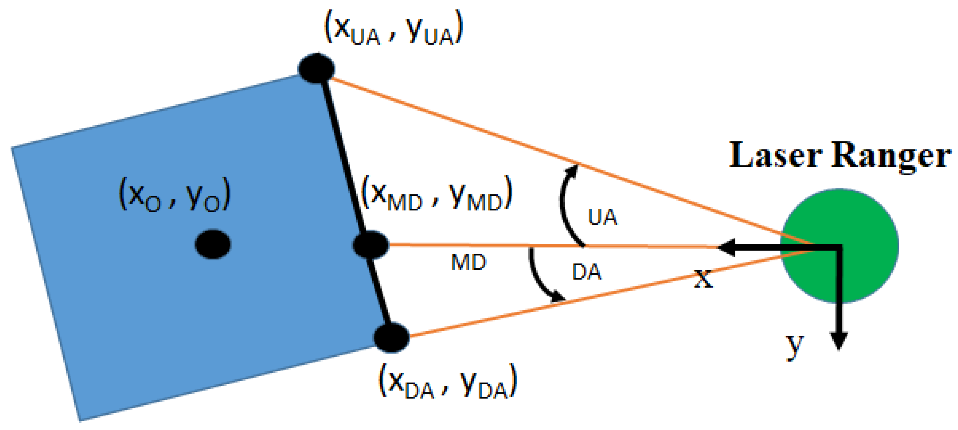
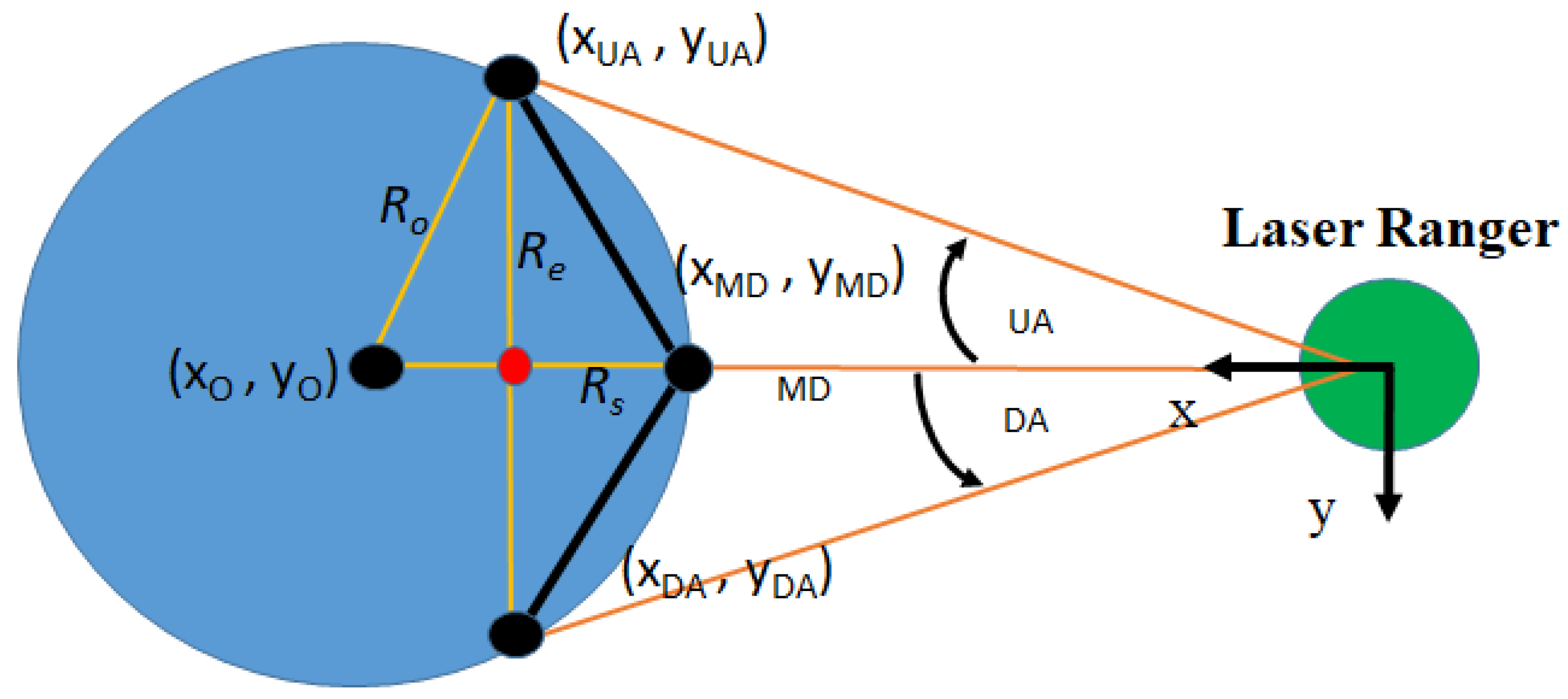
3.4. Radius Calculation of Obstacle

The obstacles are set as square and circular to facilitate identifying robots after clustering. During the laser ranger scan, the segment slope difference ( s l o p e _ d i f f ) could be calculated using the up angle (UA) point ( x U A , , y U A ) , the minimum distance (MD) point ( x M D , , y M D ) , and the down angle (DA) point ( x D A , , y D A ) , as shown in Figure 6. For a square, the shortest distance point might change, but it would be on one side of the square, and the slope difference would be small.
s l o p e _ d i f f = y U A y M D x U A x M D     y M D y D A x M D x D A
Figure 7 shows the design of circular obstacles. Since the signal from the 2D laser ranger is emitted 360 degrees around its center point, the shortest distance between two points is the connection distance between the two center points minus the radius of the two circles.
By subtraction of the slope, if the value is between minus 0.2 and plus 0.2, it is determined that the obstacle is a square; otherwise, a circle is drawn as in (3).
f x =   n o t     c i r c l e ,   0.2 > s l o p e d i f f > 0.2   c i r c l e ,                         e l s e                                                    
The Pythagorean theorem can be used to solve a quadratic equation in one variable if it is in the form of a circle. The radius of an obstacle is represented by the unknown number R o . R e is the length by the position of the point cloud with the maximum angle of the point, and the distance to the point cloud with the minimum angle divided by two. R s is the point cloud with the shortest distance, the middle value between the maximum and minimum angles. Therefore, solve (4–7) to obtain the Ro length.
R o 2 = R e 2 + R o R s 2
R o 2 = R e 2 + R o 2 2 R o R s + R s 2
2 R o R s = R e 2 + R s 2
R o = R e 2 2 R s + R s

3.5. Velocity Estimation of Moving Obstacle

As a traditional method for determining the velocity information of the moving obstacle, we attempt to differentiate the positional information of the sensors. Nonetheless, it can be measured, but if there is a noise effect, it will add to offset errors and divergence of differentiated values. Eventually, the accumulated differential variables will affect the actual velocity observed. Therefore, in this paper, we use the Kalman filter [25] to estimate an obstacle’s velocity information instead of the differential method. The Kalman filter has the advantage of filtering out noise or disturbed measurements from the sensor. Since the Apollo program of NASA in the United States in the twentieth century, the Kalman filter has been extensively studied in self-driving, positioning, and tracking. The following sections illustrate the state and observation models used in this study, the state transition matrix calculation, and the estimation process.

3.5.1. Kalman Filter Modeling

The estimation method requires two models: a predicted state for the system at the previous time, which can be represented in (8), and the sensor measurement value at the current time, which can be represented in (10)
x k = A x k 1 + B u k 1 + w k
The estimated noise w k is an independent normal probability distribution represented in (9)
p w ~ N 0 , Q
In the measurement state equation, such as in (10), Z k is the measurement state, H is the measurement matrix, and vk is the measurement noise.
Z k = H x k + v k
The measurement noise v k follows a normal probability distribution, as shown in (11)
p v ~ N 0 , R

3.5.2. Linear Acceleration Model

Assuming that the obstacle is in constant acceleration motion, the system state vector is expressed as in (12)
1 0 Δ t 0 Δ t 2 2 0 0 1 0 Δ t 0 Δ t 2 2 0 0 1 0 Δ t 0 0 0 0 1 0 Δ t 0 0 0 0 1 0 0 0 0 0 0 1
In the process of system estimation, noise covariance is defined as in (13).
Q = σ w x 2 0 0 0 0 0 0 σ w y 2 0 0 0 0 0     0 σ w v x 2 0 0 0 0 0 0 σ w v y 2 0 0 0 0 0 0 σ w a x 2 0 0 0 0 0 0 σ w a y 2
To estimate the velocity of the obstacle, we apply the constant acceleration motion model, which is expressed as x-coordinate, y-coordinate, x-velocity, y-velocity, x-acceleration, y-acceleration of the obstacle in sequence, and Δt is the time since the previous state until the current state. As a consequence, the input of the observation model is the center position of the point cloud after clustering, and its coordinates x, y serve as the design reference of the observation matrix and are shown in (14).
H = 1 0 0 0 0 0 0 1 0 0 0 0
In the observation process, the noise covariance matrix is calculated as the weighting of the state correction based on the current state and the observed noise. As the measurement noise covariance is a result of the observation noise, the diagonal line is the slope variance of the X and Y coordinates and can be defined as in (15).
R = σ v x 2 0 0 σ v y 2
It is necessary to set the initial parameters before performing the Kalman filter, as shown in the following Table 1.

3.5.3. Process Update of Kalman Filter

  • The Kalman filter prediction estimate:
    x ^ k | k 1 = A x ^ k 1 | k 1
where x ^ k | k 1   represents the prior estimate of the state, and x ^ k 1 | k 1 represents the posterior estimate at the previous moment.
P k | k 1 = A k P k 1 | k 1 A k T
where P k | k 1 represents the prior estimated covariance of the true value and the estimated value, AT is represented as the transposed matrix of A, and the smaller the Q value, the higher the trust in the model estimate.
  • Correction error for Kalman filter:
  K k = P k | k 1 H k T H k P k | k 1 H k T + R k 1
In this step, the Kalman gain K k is used to correct the results of the predicted state and measured value of the system, where H k   is the observation model, H k T is the transposed matrix of H k , and R k is the measurement noise.
    x ^ k | k = x ^ k | k 1 + K k ( z k H k x ^ k | k 1 )  
In (19), x ^ k | k is the posterior estimation state, A reflects the difference ( z k H k x ^ k | k 1 ) between the two estimates, and a residual ( z k H k x ^ k | k 1 ) value of 0 signifies that the estimates are identical.
P k | k = I K k H k P k | k 1
where P k | k represents the posterior estimated covariance, which is updated as the parameter of (17).

4. Velocity Obstacle Layer Creation

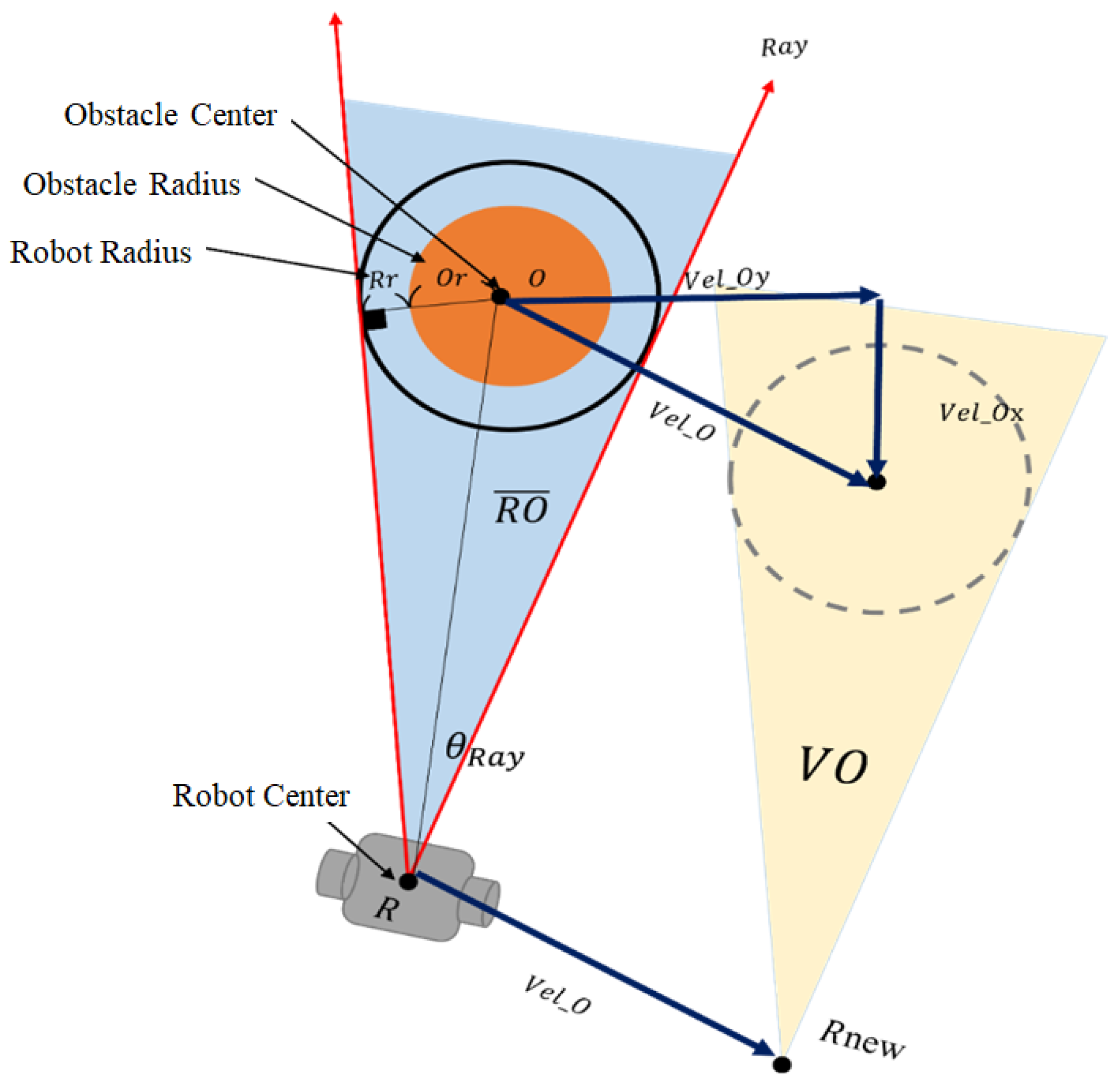
4.1. Velocity Obstacle Area

A velocity obstacle area is a place where the robot can navigate freely without encountering any obstacles. As shown in Figure 8, the yellow triangle on the right indicates impassable directions so that the robot can navigate safely and avoid obstacles. However, redundant path constraints waste many possible paths, in addition to making the walking path longer and causing movement jitter. Consequently, we will discuss the VO design process in this subsection, along with innovative cut-off distances and cut-off regions for solving past VO design problems.
According to Figure 8, the orange circle represents an obstacle, the radius of the obstacle is O r , the center point of the obstacle is O c , and the radius of the robot is   R r . By pressing R r , it will expand the orange obstacle into a black circular area. The robot and the obstacle will collide when the center of the robot enters the black circular area. Therefore, to obtain a safe area during navigation, it is only necessary to remove all the vectors in the direction of the black circle in the center of the robot. It is, therefore, sufficient to remove all the vectors in the direction of the black circle in the robot’s center to obtain a safe area during navigation.
Step 1: Calculate the angle between the robot’s coordinate and the obstacle center.
θ R O c = arctan ( O y R y / ( O x R x ) )
Step 2: Calculate the angle between the ray and   R O c
θ R a y = arcsin O r + R r D i s R O
Step 3: As a result of subtracting and adding the angles calculated in the first and second steps, we can calculate the angles of the left and right rays, as well as the sine and cosine functions for determining the x and y directions of the rays. The direction of a ray is represented by the extension of these two vectors.
θ L e f R a y = θ R O c + θ R a y    
θ R i g R a y = θ R O c θ R a y    
Considering that the obstacle itself moves at a certain speed, the robot will not collide with the blue area calculated at first, but the light yellow area that translates with the speed of the obstacle. Therefore, we add the blue triangle area to the velocity x and y direction components of the obstacle to obtain a new light yellow area, which produces the velocity obstacle area VO. The robot coordinate point R moves to the following formula of   R n e w , where the speed of the obstacle itself is represented by V e l _ O , and the x and y components of V e l _ O are V e l _ O x and V e l _ O y .
As shown in Figure 9, when VO establishes an area, it is now necessary to calculate the truncated velocity obstacle area tVO. The truncated tVO allows the robot to have more velocity vectors that can be filtered. Furthermore, the obstacle will not be hit within the cut-off time τ , and this value is greater than or equal to 1. When the time is equal to 1, which means no cut-off is carried out, and the longer the time, the shorter the cut-off distance.
Based on the following assumption, the VO area can be scaled according to time, in which the robot and the obstacle are connected by a vector R O c , the length of R O c being the distance between the robot and the obstacle, and the direction of R O c   being the angle of the robot towards the obstacle. If the robot moves according to the speed of the R O c vector, it will eventually and inevitably collide with the obstacle at the next moment, but if the R O c vector is divided by 2, it means that the robot will take twice as long to collide with the obstacle. As a result, it is possible to control the multiple time τ and truncate the length of the R O c   vector by dividing it by τ. The original gray dotted circle has a radius of r + R r , which will also be reduced by time τ to generate a black dotted circle. After that, divide (RO) by τ as the new center, and its radius is O r + R r   divided by τ, and the radius can be used to produce a circle and tVO can be obtained.

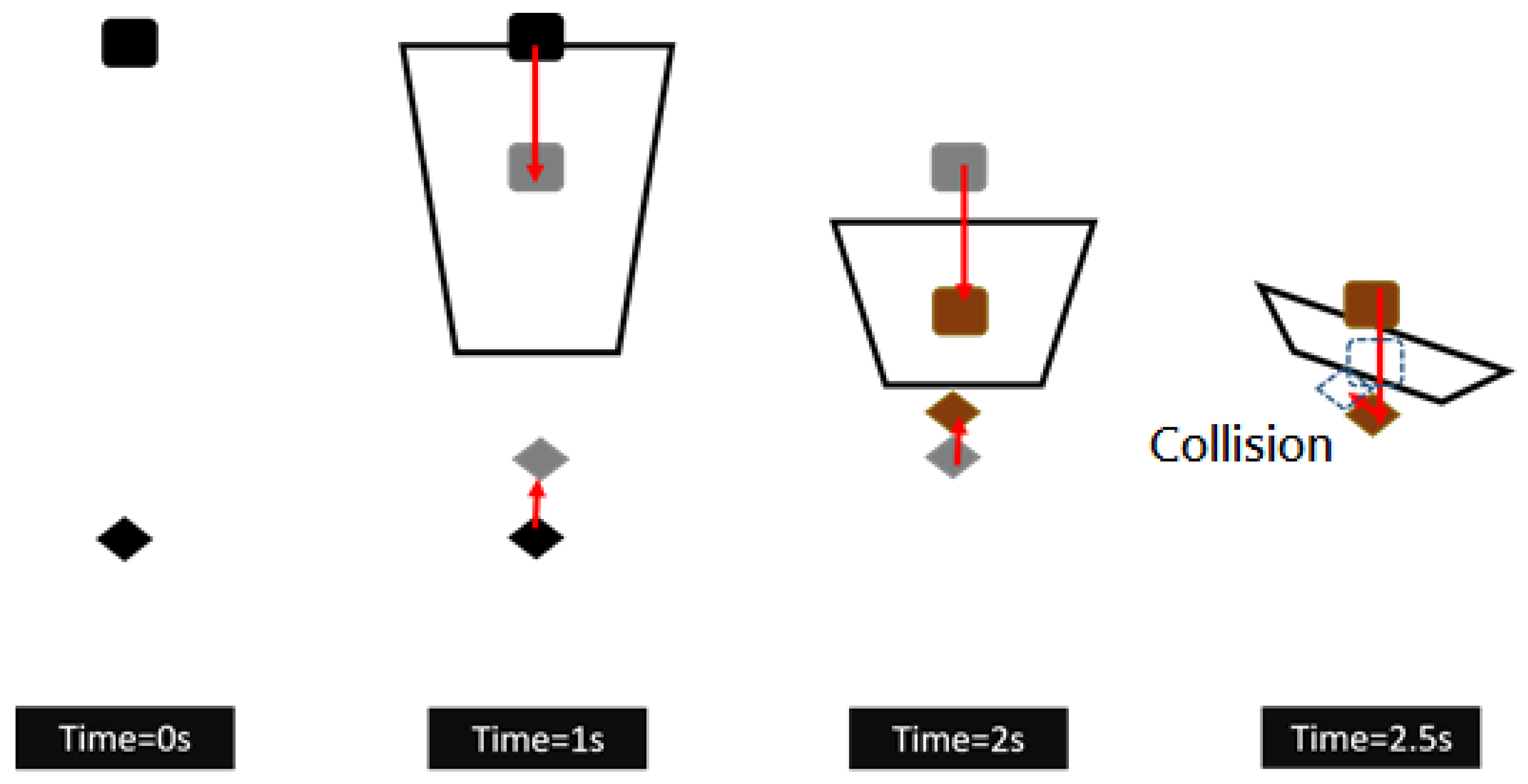
4.2. The Problem of Velocity Obstacles

Based on the velocity obstacle area algorithm and the cut-off distance formula, the robot can avoid obstacles in the navigation path. In contrast, if the robot and the obstacle have a different travel speed or the obstacle is not designed with a cut-off distance, they may collide within its obstacle area. We will analyze the feasibility of obstacle avoidance by explaining the movement sequence of the robot and explaining the innovation of improving the truncation area of the velocity obstacles.
Figure 10 shows two robots moving forward simultaneously, and their speeds are 0.1 and 0.3 m/s, respectively. At time T = 1, if the diamond-shaped robot does not enter the black trapezoidal area and the square robot does not enter the yellow trapezoidal area, then it can safely avoid obstacles in the velocity obstacle cut-off area. At T = 2, the square robot makes a right dodge decision due to detecting the yellow trapezoidal area as impassable, which allows the diamond-shaped robot to continue to move forward. They can finally safely dodge each other when T = 3.
Conversely, if only the robot follows the truncated area, a collision is likely to occur when encountering a high-speed obstacle. As shown in the Figure 11 below, assuming 0.3 m/s is the maximum speed of the square obstacle and 0.1 m/s is the maximum speed of the diamond robot, they move forward according to the speed obstacle area algorithm and the cut-off distance formula. As long as the diamond-shaped robot does not enter the black trapezoid, safety is assured. However, when T = 2.5, because the obstacles continue to move forward, the robots find that they may collide with each other and need to dodge. Due to the influence of the maximum velocity limit, the robots collide. As a result, if there is only a single robot run for obstacle avoidance, it is necessary to adjust the cut-off distance for velocity obstacles to avoid collisions.

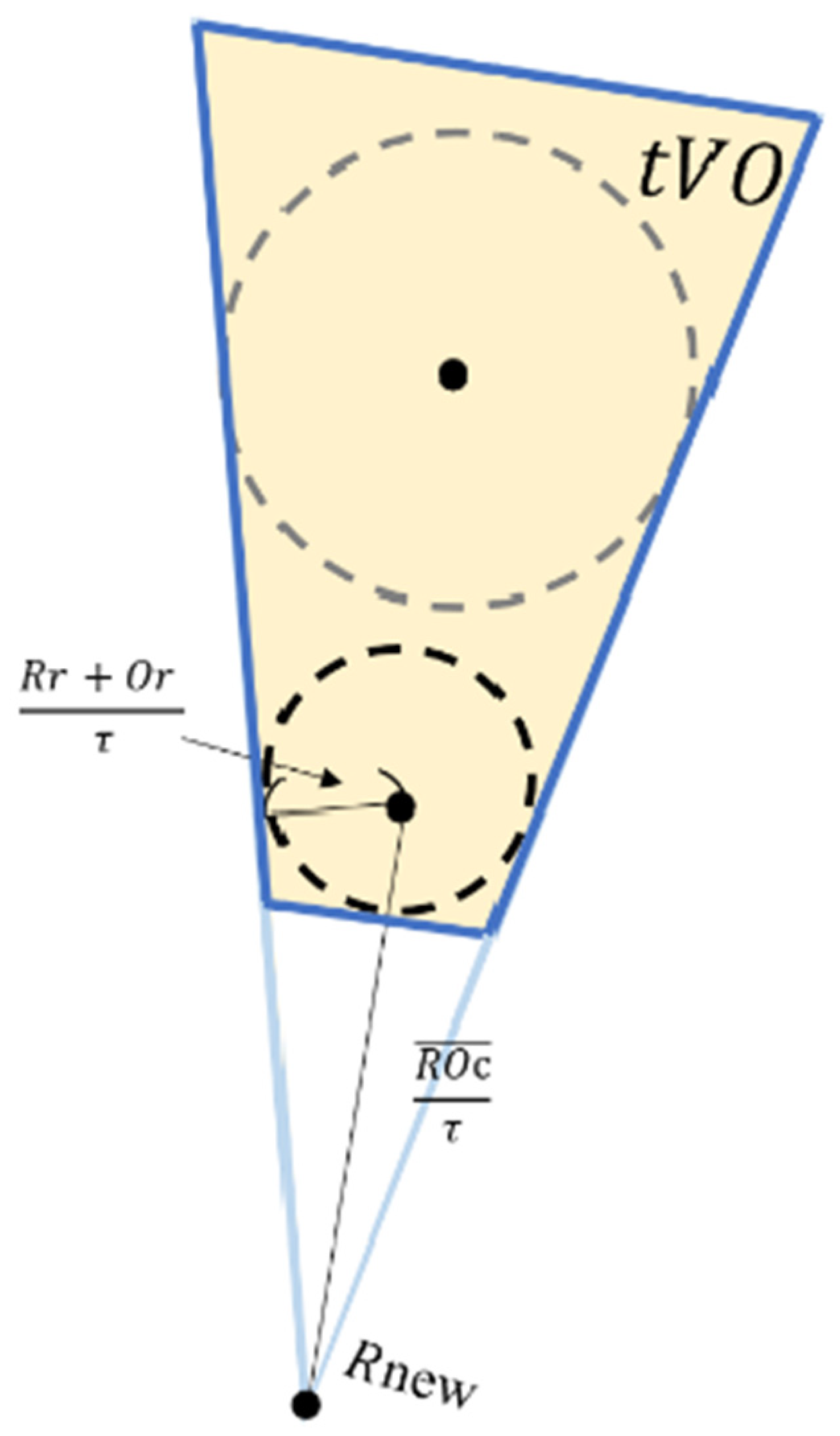
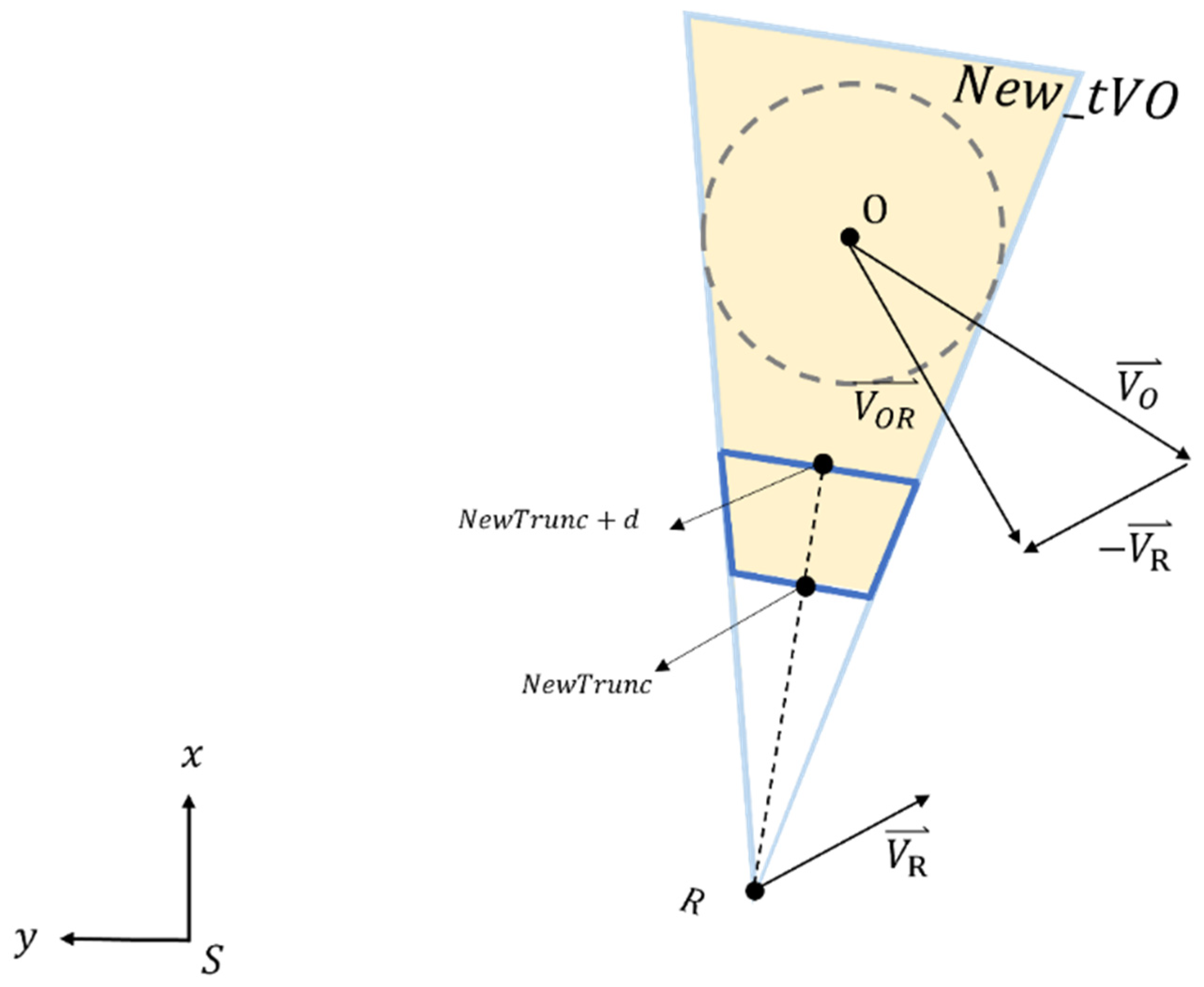
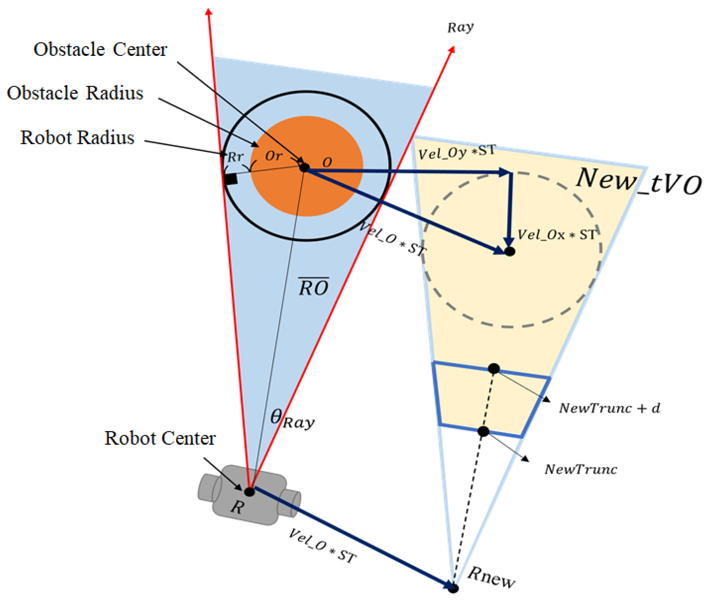
4.3. Truncation area Enhancement

If the obstacle’s velocity is high enough, the robot needs to consider its velocity and make a new obstacle avoidance strategy. In this paper, we improve the design of the truncation area and add the relative velocity between the robot and the obstacle. Figure 12 shows that the relative velocity of the robot and the obstacle is projected onto the vector of the obstacle towards the robot. We can determine the new distance for the ball segment by scaling the distance from the obstacle to the robot   D i s R O with the velocity of its projection.
P R = S R    
P R represents the vector of the robot’s starting position relative to its current position.
P O = S O    
P o represents the vector of the robot’s starting position relative to its current position
t ^ = P R P O   R O ¯    
t ^ represents the unit vector of the obstacles to the robot’s coordinates
n e w T r u n c = R O ¯   × 1 V O R · t ^ V m a x    
The new cut-off distance has been designed to consider velocity and project the velocity barrier area into the cost map, and obstacle velocity V e l _ O will not be added directly to the cost map since it is in the spatial domain. Within the regional planning algorithm, the obstacle velocity is multiplied by the sampling time of the velocity command. By converting the velocity into the spatial domain, the regional path planning algorithm may be able to avoid this cost map. Afterward, the robot will compute a new decision strategy based on the truncation distance with the velocity, and it will avoid the obstacle. For simulation and verification, the dynamic window method will be used as a local planning algorithm, and the translation calculation will be embedded in the cost map, as shown below and in Figure 13.
s h i f t x = V e l O x · S T
S T is the sampling time of the local path planning algorithm.
s h i f t y = V e l _ O y ·   S T

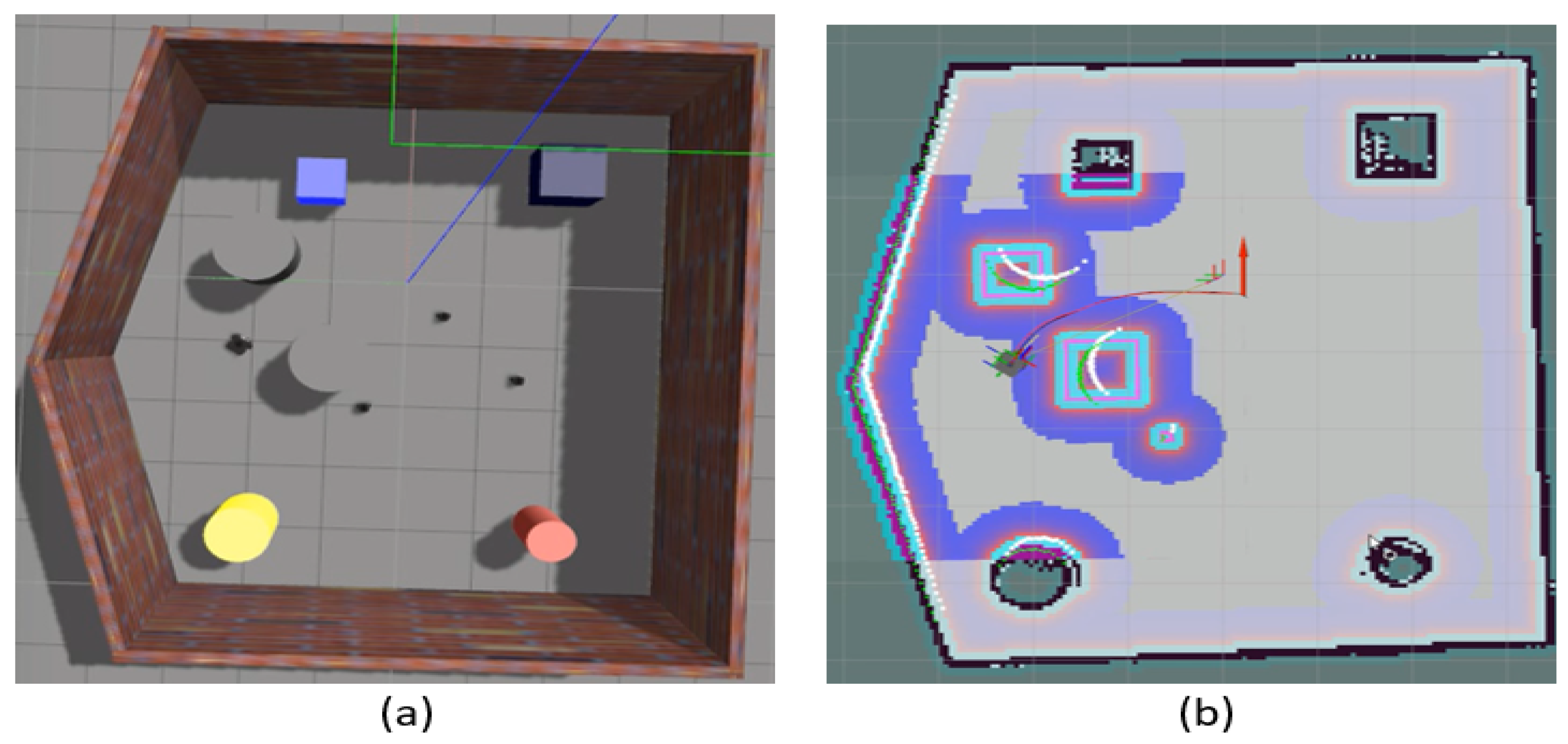
5. Experimental Results

To verify the navigation of the robot with the dynamic obstacle avoidance, the different experiments of not including and including the velocity obstacle layer are simulated and implemented in this section, and DWA is used as the local path planning method.

5.1. Default Dynamic Obstacle Avoidance

In this experiment, a robot will be designed in a simulated environment to show dynamic obstacle avoidance behavior based on the traditional cost map layer for DWA. This simulated environment contains a round robot and an obstacle, which move toward each other at a speed of 0.1 and 0.3 m/s, respectively. The figure below shows the obstacle avoidance behavior of the traditional obstacle layer.
Figure 14a shows a round d robot and a columnar obstacle in a simulated environment. The red arrow indicates the robot’s position and direction, and the black solid line is its path planning as they move toward each other. According to Figure 14b, since the sensor judges that there is an obstacle ahead, the robot cannot pass smoothly, so a new black solid line global path is determined. A difference in speed has already brought the upper obstacle close to the lower robot.
As shown in Figure 14c, since the robot’s laser sensor detects a moving obstacle ahead, it will determine that it is a static obstacle at this time. As a result of the robot’s inability to determine the obstacle’s direction and the obstacle’s velocity, the path planner cannot plan a path to avoid obstacles in advance.

5.2. VO for Dynamic Obstacle Avoidance

Figure 15 shows the simulated environment replaced by adding the velocity obstacle layer. According to the same experimental design, the robot and obstacle move toward each other. When the upper column obstacle moves forward, the robot will create a new cost map layer of velocity obstruction with moving obstacles, which is the blue trapezoidal block in Figure 15b.
Due to the design of the newly created velocity obstacle layer in Figure 15c, the real-time space environment obstacles are covered, allowing a safe path to be planned between a robot and an obstacle within a certain distance. With the new design of the velocity obstacle layer, Figure 15d shows that the robot can effectively avoid obstacles three times faster than it by using the local path planner, enabling us to achieve safe obstacle avoidance through the shortest possible distance of only 0.6 m.

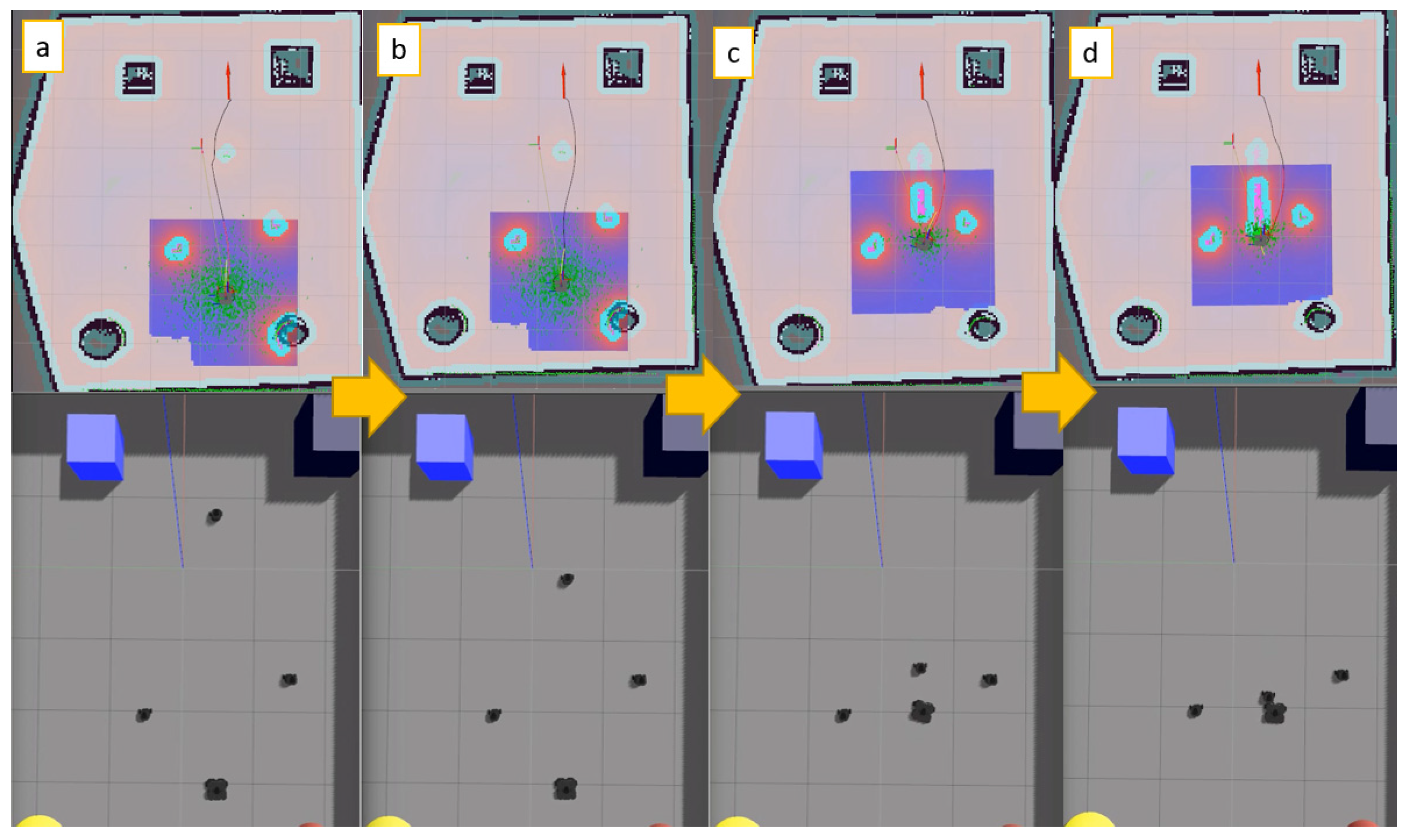
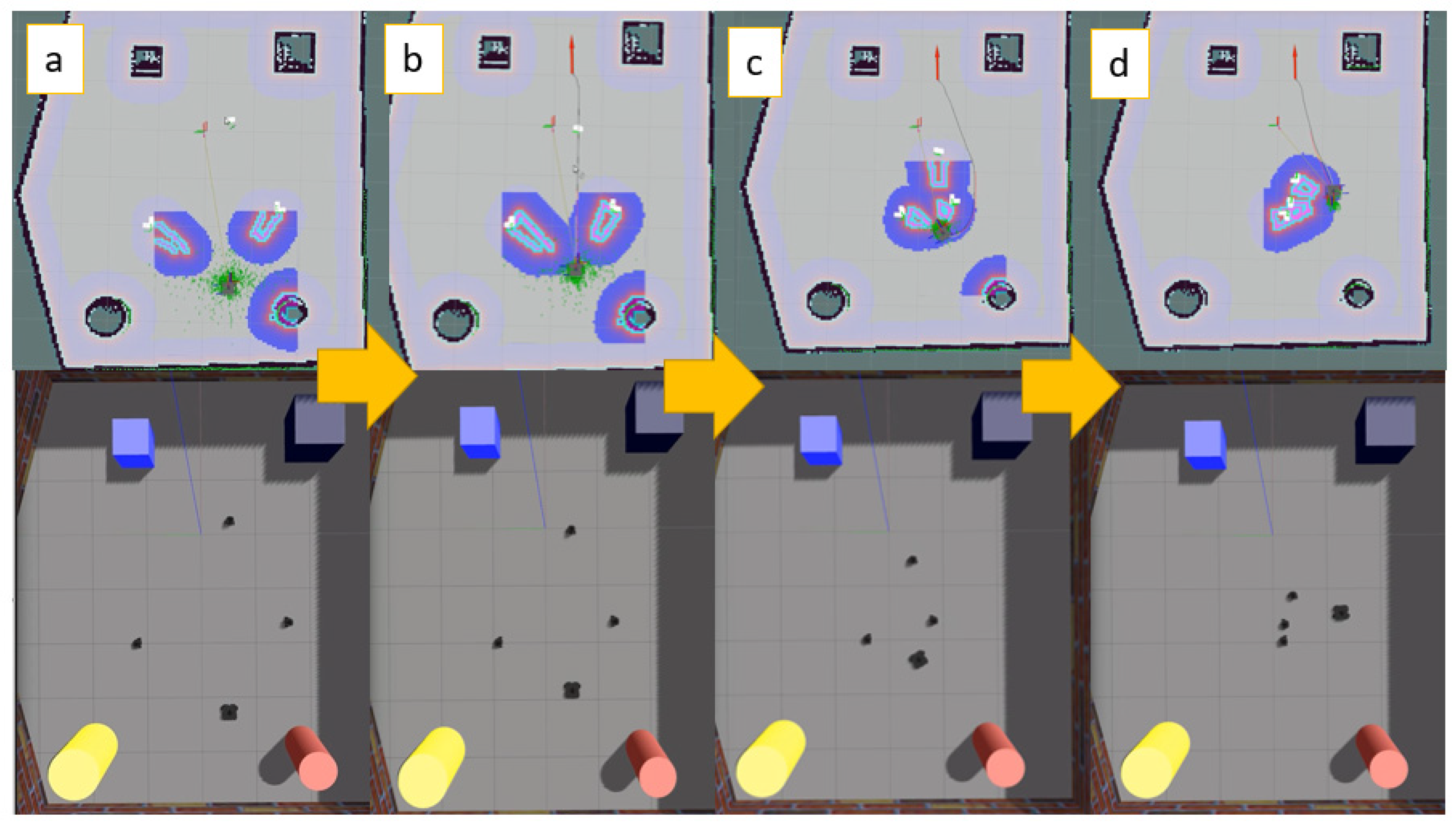
5.3. Multi-Dynamic Obstacle Avoidance with VO

In addition to simulating a single obstacle above, the velocity obstacle layer can actually be applied to multiple dynamic obstacle avoidance. In this simulated environment, we pre-defined three movable obstacles, which are located on the robot’s front, left and right sides. The subfigures a–d of Figure 16 illustrate the obstacle avoidance process of the robot, the upper part shows the visualization of the velocity obstacle layer, and the lower part shows the robot’s simulated environment.
The obstacles in Figure 16a, approach the robot at a high speed, respectively, and the new VO layer is generated by real-time estimation. Due to the determination of the VO layer, the robot is expected to collide in Figure 16b. The robot generates a new obstacle avoidance path when three obstacles approach at a high speed in Figure 16c. Finally, we can see that the robot successfully avoided the three obstacles without colliding due to the effective collaboration between the velocity obstacle layer and the path planner in Figure 16d.

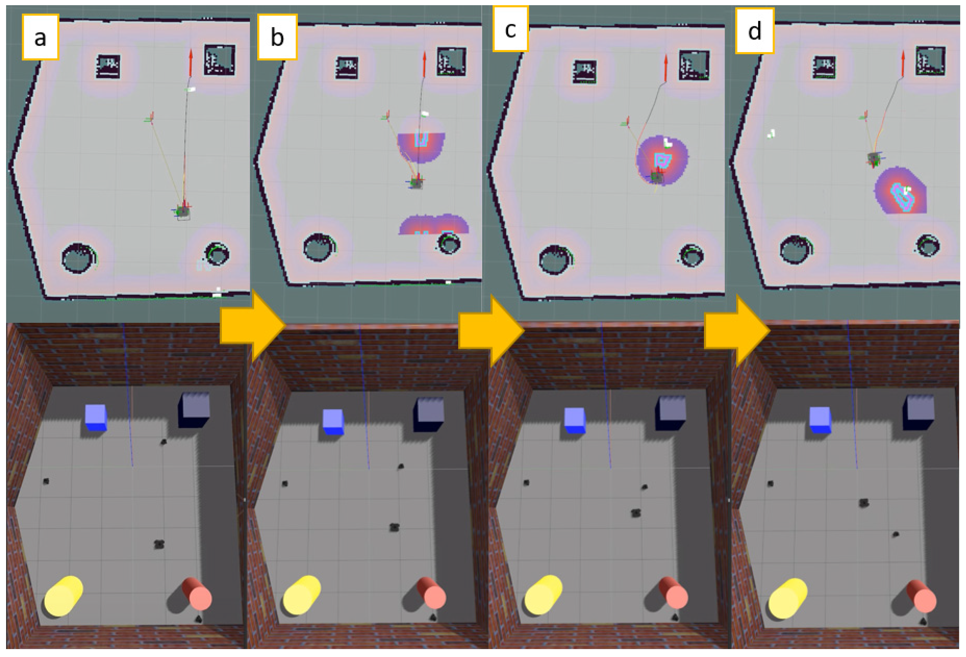
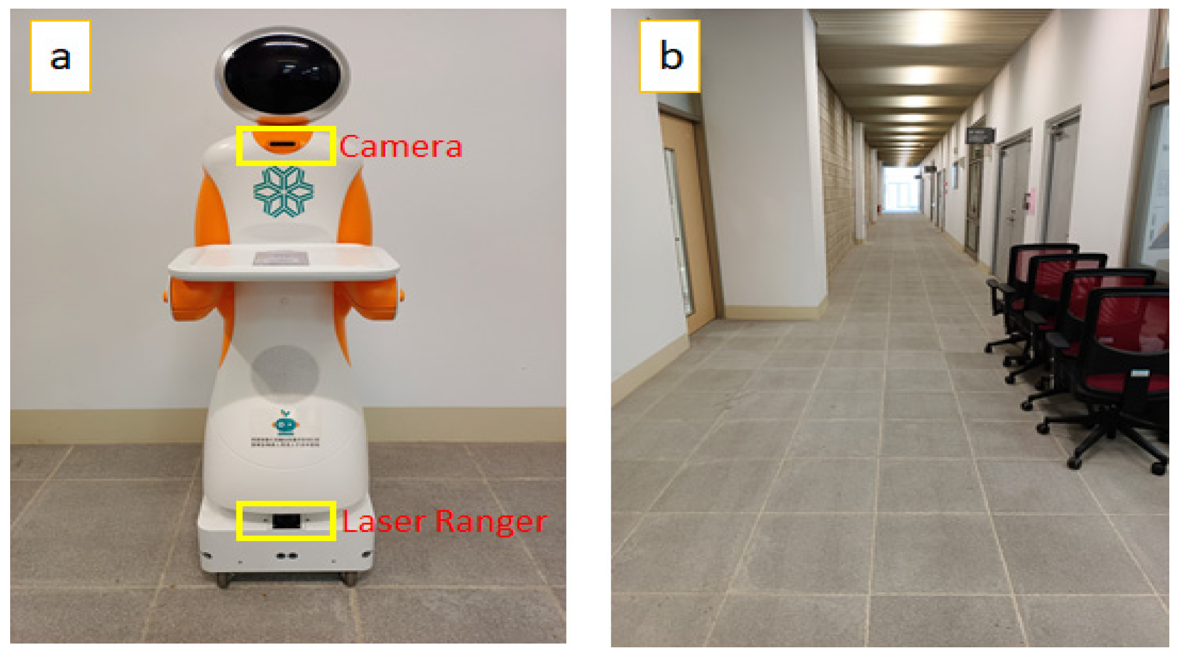
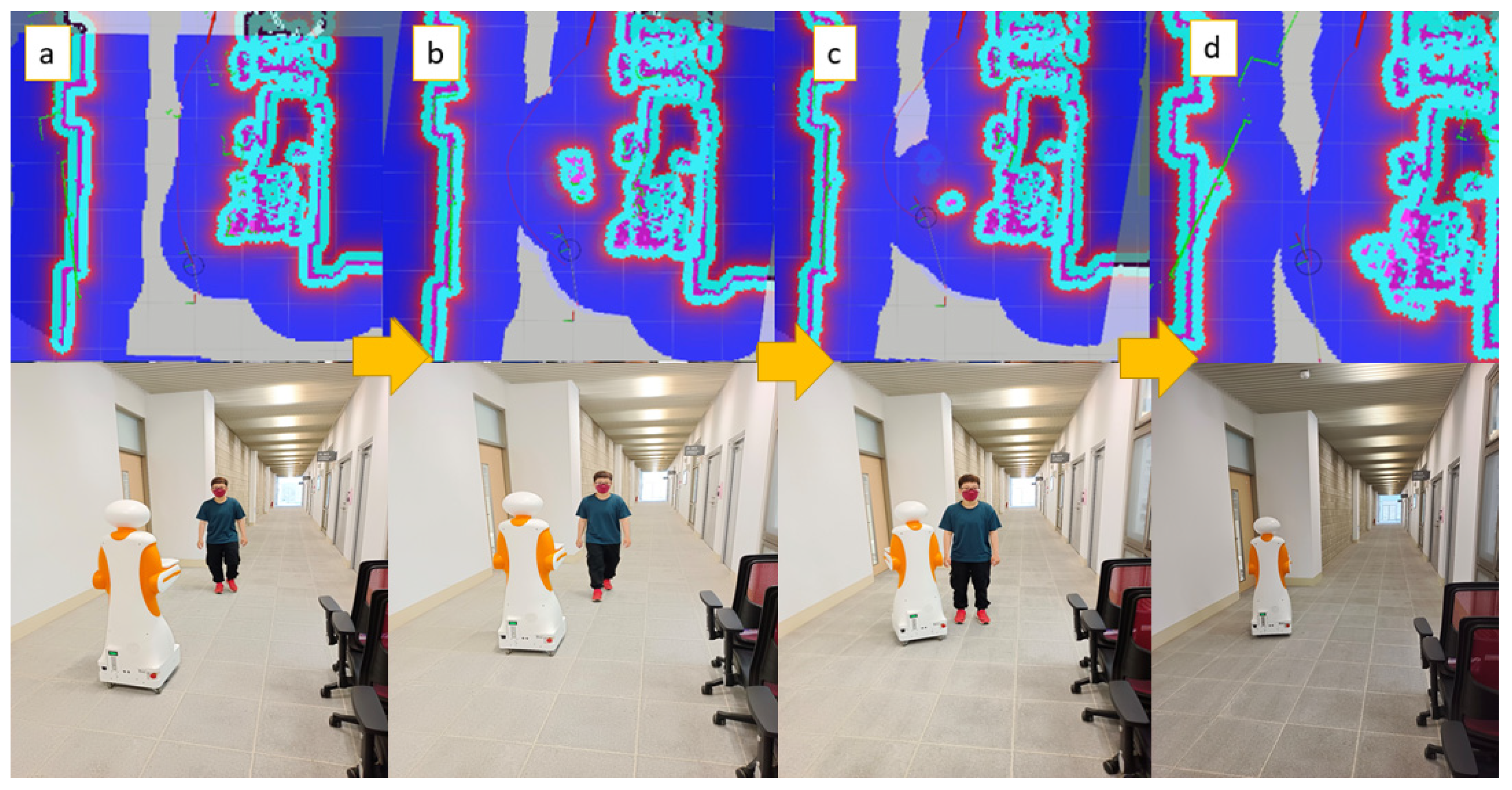
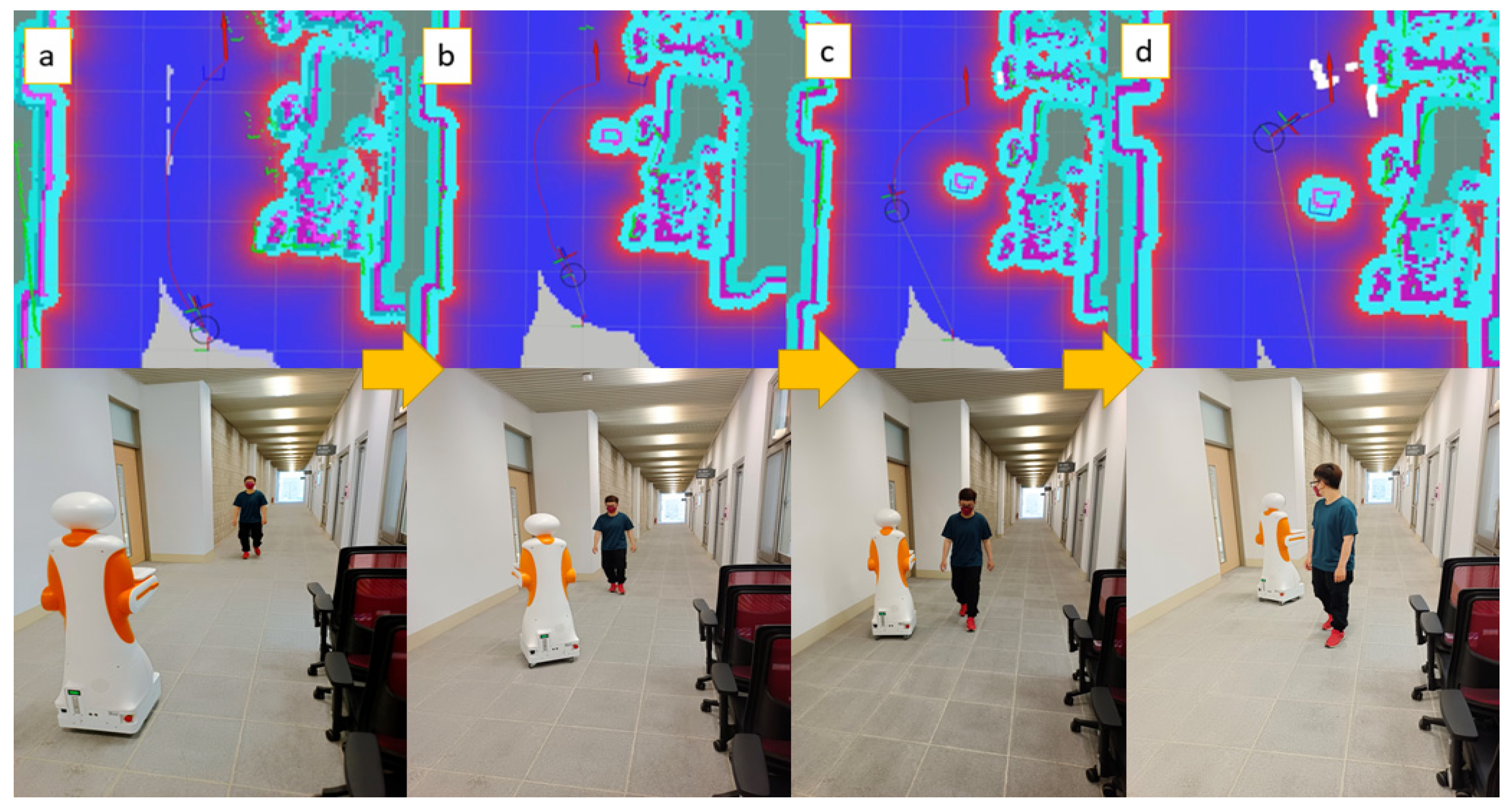
5.4. Actual Dynamic Obstacle Avoidance

The simulated environments shown above were used for verifying the obstacle avoidance performance with the velocity obstacle layer. In practice, people will be used as dynamic moving obstacles and verified through a robotic platform. Figure 17a shows that the robot is a differential wheel mobile platform, with the 2D laser ranger in the lower region and the depth-of-field camera in the upper region. There are environmental obstacles in the experimental field for the robot to avoid within a limited space, as shown in Figure 17b. The actual experiment field has a width of 2.7 m and a length of over 6 m.
Figure 18a,b shows that the obstacle is moving faster than the robot. After the cost map mechanism generates environmental obstacles, although the local path planner DWA attempts to plan an obstacle avoidance path, they still collide due to the lack of time. Figure 18c shows that when an obstacle avoidance failure occurs, ROS_move_base starts the rotation recovery process when the robot collides. As a result of the positioning offset before path planning, the robot is forced to stop its navigation and clear the original cost map. Experimentally, when colliding with a dynamic obstacle, a rotation recovery means that the robot cannot reach its original target point in time, requiring additional navigation time.
On the other hand, as shown in Figure 19, the real field testing obstacle avoidance process was implemented using the velocity obstacle layer as the robot application. In the experiment, the robot and a person are moving toward each other. A robot that observes a moving obstacle can add velocity information to the velocity obstacle layer in real-time and pass it to the local path planner. Figure 19b,c shows how this works. The planner generates the arc-shaped blue trajectory to avoid obstacles.
Even though the pedestrian continues to move faster than the robot, the green laser ranger point cloud and the coordinates of the robot tell us that the robot and the pedestrian keep a safe distance from one another. Finally, Figure 19d shows that the robot successfully avoided the dynamic pedestrian and reached the target point to complete the obstacle avoidance task. By using the VO cost map layer, the robot’s obstacle avoidance mechanism can be successfully combined with the DWA local path planner.

5.5. Performance Comparison

The experiments in the real environment are compared with the number of successful obstacle avoidances, the total time spent, the total length of the path, and the distance to the closest obstacle without adding the velocity obstacle layer versus adding the velocity obstacle layer. There is a time comparison in Table 2 of the overall time spent, as the DWA algorithm will make the robot start the recovery behavior when the obstacle is too close to the robot. There is a time benefit to the navigation process when the VO cost map layer is added since the obstacle can be avoided smoothly in advance.
The navigation distances are shown in Table 3, and the average path of the method adding the velocity obstacle layer is longer. Due to the VO layer calculating a safer and more conservative speed obstacle area between the robot and the obstacle, the path length for obstacle avoidance will be longer.
By adding the velocity obstacle layer, the robot maintains a very safe distance from the pedestrian during the obstacle avoidance process since the velocity vector of the pedestrian is taken into account. On the other hand, the distance between the robot and human is significantly smaller in the method without adding the velocity obstacle layer, as shown in Table 4.

6. Discussion and Conclusions

In this study, the Kalman filter is used to estimate the moving velocity of dynamic obstacles, and the cost map of ROS is enhanced with a velocity obstacles layer to evaluate the difference between the dynamic obstacle avoidance of the robot using the velocity obstacle layer based on simulated and actual environments.

6.1. Simulation and Implementation

As a result of the experiments, without the velocity obstacle layer, the obstacle cannot be detected in time on the cost map and the obstacle occupies the navigation end point, the system activates the cost map cleaning mechanism, and the robot’s positioning fails due to in-situ rotation behavior. Similarly, because of the time delay between the generation of obstacles and the cost layer, the distance between the obstacles and the robot is close, which may cause a collision. This paper proposes a velocity obstacle layer method that observes the velocity of obstacles. Not only can the cost map for obstacles be updated in real-time, but it also prevents the end position from being occupied during the navigation. In addition, the cut-off distance proposed in this study takes into account the speed of moving objects so that the robot can maintain a safe distance of at least 0.46 m, which ensures the stability of the robot when encountering dynamic obstacles.

6.2. Computation Resources

In this experiment, the Intel® Core™ i5-5200U mini PC and D435i RealSense camera are used for dynamic object recognition and tracking. The VO dynamic obstacle avoidance simulation control environment is tested on the ASUS TUF DASH F15 laptop, the computing resources include Intel processors 3.3 GHz, 4 cores, and a Ubuntu 20.04 operating system. More than 10 Hz can be achieved in a robot navigation control loop. This actual robot system is controlled by an NVIDIA Jetson TX2, and the actual rate of the system control loop is 8 Hz.
In addition, the calculation amount of DeepSORT is 0.23Bflops (Billion float operations) per second (Floating Point Operations Per Second, FLOPS). The mAP (mean average precision) in the Visual Object Classes Challenge 2017 (VOC2017) data is about 61%. Although the experiment does not rely on the GPU, it can also show a good performance of about 10 FPS. In the future, the GPU can be integrated into the robot platform to improve tracking performance and real-time control capability, allowing for real-time obstacle detection and avoidance.

6.3. Contribution and Future Work

The main contribution of this study is the improvement of the cut-off distance calculation through velocity obstacle cost maps and relative velocities of obstacles. We optimize the navigation performance of the robot when it encounters high-speed moving obstacles and perform the actual field testing of the mobile robot based on ROS. According to the experimental results, the improved velocity obstacle cost map layer allows the robot to avoid dynamic moving obstacles faster and more safely. It can improve the determination of the original obstacles as well as the smoothness of the path planning process. As a result of this study, robot motion is significantly improved, and dynamic obstacles are effectively avoided.
With the result, this research experiment can accurately estimate pedestrians or robots at a high speed for obstacle avoidance in robot navigation, but the social behavior between crowds is not in this scope. In the future, the artificial network model should be combined with long-term memory to train the trajectory of encountering pedestrians in different situations to enhance the robot’s obstacle avoidance flexibility when encountering pedestrians with the innovative design of VO and implementation in ROS-based AMR.

Author Contributions

Conceptualization, C.S.C. and C.J.L.; methodology, C.S.C. and S.Y.L.; software, S.Y.L.; validation, C.J.L. and C.C.L.; formal analysis, C.S.C.; investigation, C.J.L. and C.C.L.; re-sources, C.S.C.; data curation, S.Y.L.; writing—original draft preparation, S.Y.L. and C.J.L.; writing—review and editing, C.J.L. and C.C.L.; visualization, C.J.L.; supervision, C.C.L.; project administration, C.S.C.; funding acquisition, C.S.C. All authors have read and agreed to the published version of the manuscript.

Funding

This study were financially sponsored by the Ministry of Science and Technology under project No. MOST 109-2221-E-027-044 -MY3 and 110-2410-H-224-038.

Institutional Review Board Statement

Not applicable.

Informed Consent Statement

Not applicable.

Data Availability Statement

The data presented in this study are available upon request from the corresponding author.

Conflicts of Interest

The authors declare no conflict of interest.

References

  1. Quigley, M.; Gerkey, B.; Conley, K.; Faust, J.; Foote, T.; Leibs, F.; Berger, E.; Wheeler, R.; Ng, A. ROS: An open-source Robot Operating System. ICRA Workshop Open Source Softw. 2009, 3, 5. [Google Scholar]
  2. Move_Base—ROS Wiki. Available online: http://wiki.ros.org/move_base (accessed on 20 May 2022).
  3. Abdelrasoul, Y.; Saman, A.B.S.H.; Sebastian, P. A quantitative study of tuning ROS gmapping parameters and their effect on performing indoor 2D SLAM. In Proceedings of the 2016 2nd IEEE International Symposium on Robotics and Manufacturing Automation (ROMA), Ipoh, Malaysia, 25–27 September 2016; pp. 1–6. [Google Scholar]
  4. Weichen, W.E.I.; Shirinzadeh, B.; Ghafarian, M.; Esakkiappan, S.; Shen, T. Hector SLAM with ICP trajectory matching. In Proceedings of the 2020 IEEE/ASME International Conference on Advanced Intelligent Mechatronics (AIM), Boston, MA, USA, 6–9 July 2020; pp. 1971–1976. [Google Scholar]
  5. Nüchter, A.; Bleier, M.; Schauer, J.; Janotta, P. Improving Google’s Cartographer 3D mapping by continuous-time slam. Int. Arch. Photogramm. Remote Sens. Spat. Inf. Sci. 2017, 42, 543. [Google Scholar] [CrossRef] [Green Version]
  6. Mur-Artal, R.; Montiel, J.M.M.; Tardos, J.D. ORB-SLAM: A versatile and accurate monocular SLAM system. IEEE Trans. Robot. 2015, 31, 1147–1163. [Google Scholar] [CrossRef] [Green Version]
  7. Zhang, L.; Zapata, R.; Lepinay, P. Self-adaptive Monte Carlo localization for mobile robots using range finders. Robotica 2012, 30, 229–244. [Google Scholar] [CrossRef] [Green Version]
  8. Zwirello, L.; Schipper, T.; Harter, M.; Zwick, T. UWB localization system for indoor applications: Concept, realization and analysis. J. Electr. Comput. Eng. 2012, 4, 1–11. [Google Scholar] [CrossRef]
  9. Kriz, P.; Maly, F.; Kozel, T. Improving indoor localization using bluetooth low energy beacons. Mob. Inf. Syst. 2016, 2016, 1–11. [Google Scholar] [CrossRef] [Green Version]
  10. Costmap_Prohibition_Layer—ROS Wiki. Available online: http://wiki.ros.org/-costmap_prohibition_layer (accessed on 20 May 2022).
  11. Duchoň, F.; Babinec, A.; Kajan, M.; Beňo, P.; Florek, M.; Fico, T.; Jurišica, L. Path planning with modified a star algorithm for a mobile robot. Proc. Eng. 2014, 96, 59–69. [Google Scholar] [CrossRef] [Green Version]
  12. Fan, D.; Shi, P. Improvement of Dijkstra’s algorithm and its application in route planning, IEEE Int. Conf. Fuzzy Syst. Knowl. Discov. 2010, 4, 1901–1904. [Google Scholar]
  13. LaValle, S.M.; Kuffner, J.J.; Donald, B.R. Rapidly-exploring random trees: Progress and prospects. Algorith. Comput. Robot. N. Dir. 2001, 5, 293–308. [Google Scholar]
  14. Fox, D.; Burgard, W.; Thrun, S. The dynamic window approach to collision avoidance. IEEE Robot. Autom. Mag. 1997, 4, 23–33. [Google Scholar] [CrossRef] [Green Version]
  15. Dechter, R.; Pearl, J. Generalized best first search strategies and the optimality of A. J. Assoc. Comput. Machin. 1985, 32, 505–536. [Google Scholar] [CrossRef]
  16. Wilkie, D.; Van Den Berg, J.; Manocha, D. Generalized velocity obstacles. IEEE Int. Conf. Intell. Robot. Syst. 2009, 2009, 5573–5578. [Google Scholar]
  17. Van den Berg, J.; Lin, M.; Manocha, D. Reciprocal velocity obstacles for real-time multi-agent navigation. In Proceedings of the 2008 IEEE International Conference on Robotics and Automation, Pasadena, CA, USA, 19–23 May 2008; pp. 1928–1935. [Google Scholar]
  18. Allawi, Z.; Abdalla, T. A PSO-optimized reciprocal velocity obstacles algorithm for navigation of multiple mobile robots. IAES Int. J. Robot. Autom. 2015, 4, 31. [Google Scholar] [CrossRef]
  19. Alonso-Mora, J.; Breitenmoser, A.; Rufli, M.; Beardsley, P.; Siegwart, R. Optimal reciprocal collision avoidance for multiple non-holonomic robots. Distrib. Auton. Robot. Syst. 2013, 83, 203–216. [Google Scholar]
  20. Liu, Z.; Jiang, Z.; Xu, T.; Cheng, H.; Xie, Z.; Lin, L. Avoidance of high-speed obstacles based on velocity obstacles. In Proceedings of the 2018 IEEE International Conference on Robotics and Automation (ICRA), Brisbane, QLD, Australia, 21–25 May 2018; pp. 7624–7630. [Google Scholar]
  21. Samsani, S.S.; Muhammad, M.S. Socially compliant robot navigation in crowded environment by human behavior resemblance using deep reinforcement learning. IEEE Robot. Autom. Lett. 2021, 6, 5223–5230. [Google Scholar] [CrossRef]
  22. Wojke, N.; Bewley, A.; Paulus, D. Simple online and real time tracking with a deep association metric. In Proceedings of the 2017 IEEE International Conference on Image Processing (ICIP), Beijing, China, 17–20 September 2017; pp. 3645–3649. [Google Scholar]
  23. Host, K.; Ivasic-Kos, M.; Pobar, M. Tracking Handball Players with the DeepSORT Algorithm. ICPRAM 2020, 593–599. [Google Scholar] [CrossRef]
  24. Hartigan, J.A.; Wong, M.A. Algorithm AS 136: A k-means clustering algorithm, J.R. Stat. Soc. 1979, 28, 100–108. [Google Scholar] [CrossRef]
  25. Welch, G.; Bishop, G. An Introduction to the Kalman Filter; University of North Carolina: Chapel Hill, NC, USA, 1995. [Google Scholar]
Figure 1. ROS “move base” navigation stack on a robot.
Machines 10 00501 g001
Figure 2. ROS cost map with multiple layers.
Machines 10 00501 g002
Figure 3. An illustration of possible collisions based on sampling in velocity space.
Machines 10 00501 g003
Figure 4. The velocity estimation and cost map generation workflow diagram.
Machines 10 00501 g004
Figure 5. Simulation results of the clustering algorithm: (a) A virtual world for robot and obstacle avoidance simulation, (b) the robot and obstacles are represented in the cost map layer.
Machines 10 00501 g005
Figure 6. Square obstacle.
Machines 10 00501 g006
Figure 7. Circle obstacle.
Machines 10 00501 g007
Figure 8. Velocity obstacle area.
Machines 10 00501 g008
Figure 9. Truncate velocity obstacles.
Machines 10 00501 g009
Figure 10. The sequence of robots avoiding obstacles interactively.
Machines 10 00501 g010
Figure 11. Schematic diagram of collision between obstacles and robots.
Machines 10 00501 g011
Figure 12. Consideration of velocity in the cutting-off distance.
Machines 10 00501 g012
Figure 13. The final velocity obstacle layer.
Machines 10 00501 g013
Figure 14. The subfigures (ad) illustrate the obstacle avoidance process of the robot in the cost map layer, the upper part of which shows the visualization tool, and the lower part shows the simulated environment.
Machines 10 00501 g014
Figure 15. The subfigures (ad) illustrate the obstacle avoidance process of the robot with the obstacle velocity layer, the upper part of which shows the visualization tool, and the lower part shows the simulated environment.
Machines 10 00501 g015
Figure 16. Multi-dynamic obstacle avoidance simulation: (a) three dynamic obstacles approach the robot in high seed, (b) the robot is expected to collide with dynamic obstacle via VO, (c) the robot updates a new path to avoid all dynamic obstacles, (d) the robot has succeeded at avoiding all dynamic obstacles.
Machines 10 00501 g016
Figure 17. The actual mobile robot and experiment field. (a) An experimental service robot equipped with laser ranger and depth camera for detecting obstacle, (b) a long and narrow walkway for the field test.
Machines 10 00501 g017
Figure 18. The subfigures (ad) illustrate the obstacle avoidance process of the actual robot without the velocity obstacle layer.
Machines 10 00501 g018
Figure 19. The subfigures (ad) illustrate the obstacle avoidance process of the actual robot with the velocity obstacle layer.
Machines 10 00501 g019
Table 1. Initial parameters of the Kalman filter.
Initial Setting of Parameters
initial position xFrom k-meaninitial acceleration ax0.0
initial position yFrom k-meaninitial acceleration ay0.0
Initial position vx0.0initial acceleration vy0.0
Table 2. Comparison of navigation time.
AVG Cost (Sec)Min Cost (Sec)Max Cost (Sec)
VO31.64 (s)26.8 (s)40.6 (s)
Non-VO41.2 (s)31.1 (s)58.6 (s)
Table 3. Comparison of navigation distance.
AVG DistanceMin DistanceMax Distance
VO5.901 (m)4.839 (m)7.534 (m)
Non-VO5.5087 (m)4.7283 (m)6.033 (m)
Table 4. Comparison of safe navigation distance.
AVG DistanceMin DistanceMax Distance
VO0.651 (m)0.463 (m)0.968 (m)
Non-VO0.284 (m)0.265 (m)0.319 (m)
Publisher’s Note: MDPI stays neutral with regard to jurisdictional claims in published maps and institutional affiliations.

