
Robust Image Matching Based on Image Feature and Depth Information Fusion


Space Optical Engineering Research Center, Harbin Institute of Technology, Harbin 150001, China
*
Author to whom correspondence should be addressed.
Machines 2022, 10(6), 456; https://doi.org/10.3390/machines10060456
Submission received: 5 May 2022
/
Revised: 27 May 2022
/
Accepted: 6 June 2022
/
Published: 8 June 2022
(This article belongs to the Topic Intelligent Systems and Robotics)
Abstract
:In this paper, we propose a robust image feature extraction and fusion method to effectively fuse image feature and depth information and improve the registration accuracy of RGB-D images. The proposed method directly splices the image feature point descriptors with the corresponding point cloud feature descriptors to obtain the fusion descriptor of the feature points. The fusion feature descriptor is constructed based on the SIFT, SURF, and ORB feature descriptors and the PFH and FPFH point cloud feature descriptors. Furthermore, the registration performance based on fusion features is tested through the RGB-D datasets of YCB and KITTI. ORBPFH reduces the false-matching rate by 4.66~16.66%, and ORBFPFH reduces the false-matching rate by 9~20%. The experimental results show that the RGB-D robust feature extraction and fusion method proposed in this paper is suitable for the fusion of ORB with PFH and FPFH, which can improve feature representation and registration, representing a novel approach for RGB-D image matching.
1. Introduction
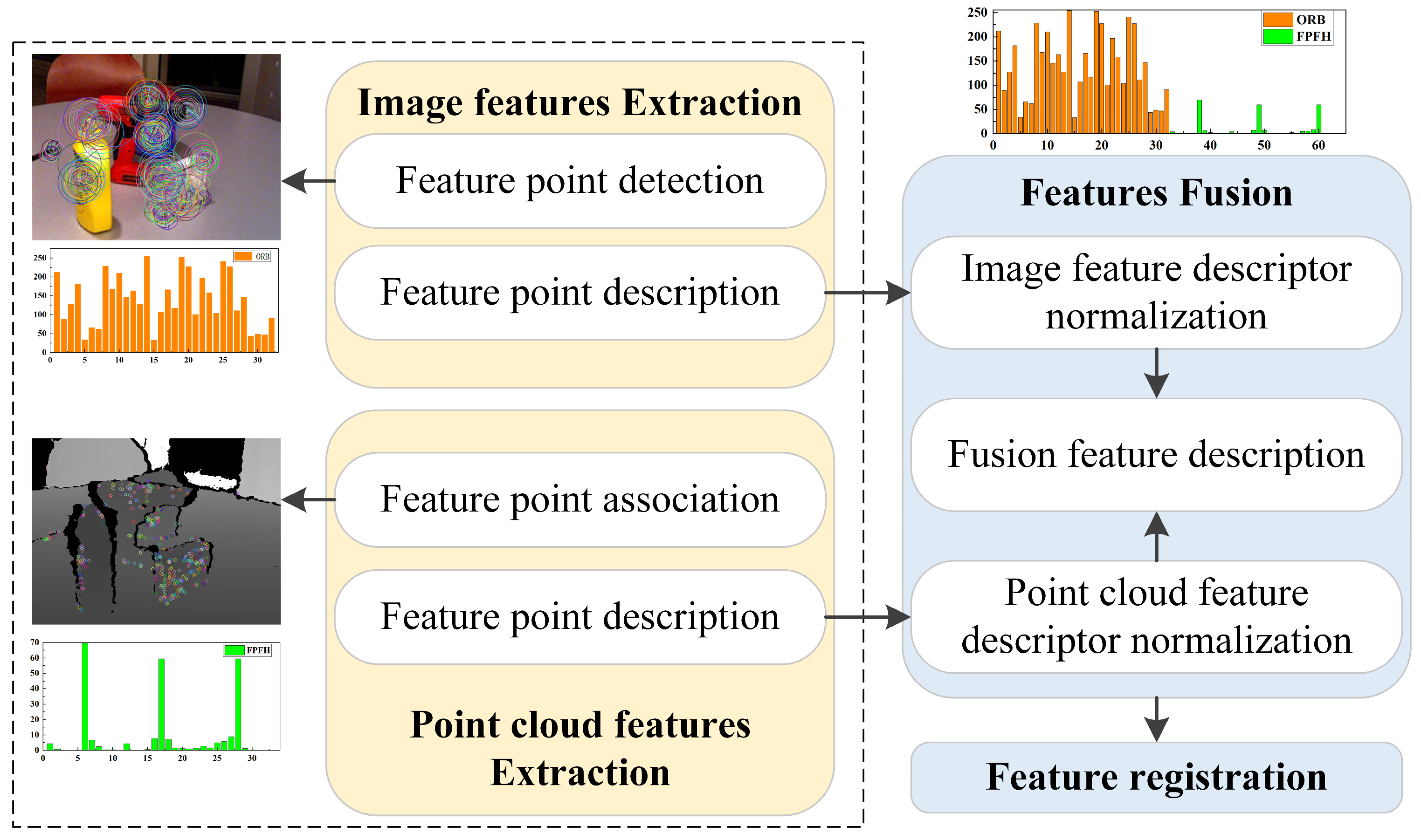
Since the advent of the Microsoft Kinect camera, various new RGB-D cameras have been launched. RGB-D cameras can simultaneously provide color images and dense depth images. Owing to his data acquisition advantage, RGB-D cameras are widely used in robotics and computer vision. The extraction and matching of image features are the basis for realizing these applications. Significant progress has been made in the feature extraction, representation, and matching of images and depth maps (or point clouds). However, there is room for further improvement of these processes. For example, the depth image includes information not contained in the original color image. Further research is required to effectively and comprehensively utilize the color image information and depth information to improve feature-matching accuracy. Therefore, to effectively fuse image and depth information and improve feature-matching accuracy, a robust RGB-D image feature extraction and fusion method based on image and depth feature fusion is proposed in this paper. The main idea of the proposed method is to directly splice the image feature point descriptor and the corresponding point cloud feature descriptor to obtain the fusion descriptor of feature points to be used as the basis of feature matching. The methodology framework comprises image feature extraction and representation, point cloud feature extraction and representation, and feature fusion, as shown in Figure 1.
The main contributions of this paper are as follows:
- A feature point description method that fuses image feature and depth information is proposed, which has the potential to improve the accuracy of feature matching.
- The feature-matching performance of different fusion features constructed based on the proposed method is verified on public RGB-D datasets.
2. Related Work
The aim of the present study is to design a robust RGB-D image feature extraction and fusion method to improve RGB-D image registration accuracy. However, a method to fully fuse RGB images with depth information remains to be established. In this section, we review current related research on feature extraction, representation, and fusion method of images and point clouds.
- (1)
- Image feature extraction and representation
Lowe et al. proposed the famous scale-invariant feature transform (SIFT) algorithm [1]. SIFT is both a feature detector and a feature descriptor. The algorithm is theoretically scale-invariant and has good anti-interference to illumination, rotation, scaling, noise, and occlusion properties. The SIFT feature descriptor is a 128-dimensional vector. However, the calculation process of this algorithm is complicated, and the speed is slow. Rosten et al. proposed the features from accelerated segment test (FAST) algorithm [2]. FAST is a corner-detection method that can quickly extract feature points. It uses a 16-pixel circle around the candidate point, p, to classify whether the candidate point is a corner. The most significant advantage of this method is high computational efficiency, but FAST is not a feature descriptor, so it must be combined with other feature descriptors. Bay et al. proposed the speeded-up robust features (SURF) algorithm [3]. SURF is a fast and high-performance scale- and rotation-invariant feature point detector and descriptor that combines the Hessian matrix and the Haar wavelet. The SURF descriptor only uses a 64-dimensional vector, which reduces the time required for feature calculation and matching. Leutenegger et al. proposed the binary robust invariant scalable keypoints (BRISK) algorithm [4]. The BRISK algorithm usually uses the FAST algorithm to detect the image’s feature points quickly, then individually samples the grayscale of each keypoint neighborhood and obtains a 512-bit binary code by comparing the sampled grayscale. BRISK has low computational complexity, good real-time performance, scale invariance, rotation invariance, and anti-noise ability but poor matching accuracy. Rublee et al. proposed the oriented FAST and rotated BRIEF (ORB) algorithm [5], which combines the FAST and BRIEF [6] algorithms, making it both a feature detector and a feature descriptor. The length of the ORB feature descriptor is generally a binary string of 128, 256, or 512. The contribution of ORB is that it adds fast and accurate direction components to the FAST and efficient calculation for the BRIEF features so that it can realize real-time calculation. However, it is not scale-invariant and is sensitive to brightness. Alahi et al. proposed the fast retina keypoint (FREAK) algorithm [7]. FREAK is not a feature detector, and it can only be applied to the keypoints that other feature detection algorithms have detected. FREAK is inspired by the human retina, and its binary feature descriptors are computed by efficiently comparing image intensities for retinal sampling patterns.
- (2)
- Point cloud feature extraction and representation
Johnson et al. proposed a 3D mesh description called spin images (SI) [8]. SI computes 2D histograms of points falling within a cylindrical volume utilizing a plane that “spins” around the normal of the plane. Frome et al. proposed regional shape descriptors called 3D shape contexts (3DSC) [9]. 3DSC directly extends 2D shape contexts [10] to 3D. Rusu et al. designed the point feature histograms (PFH) algorithm [11,12], which calculates angular features and constructs corresponding feature descriptors by observing the geometric structure of adjacent points. One of the biggest bottlenecks of using the PFH algorithm is computational efficiency for most real-time applications. In order to improve the calculation speed, Rusu et al. developed the fast point feature histogram (FPFH) algorithm [13], which is a representative, handwritten 3D feature descriptor. It provides similar feature-matching results with reasonable computational complexity. Tombari et al. proposed a local 3D descriptor for surface matching called the signature of histograms of orientations (SHOT) algorithm [14,15]. SHOT allows for simultaneous encoding of shape and texture, forming a local feature histogram. Steder et al. developed normal aligned radial feature (NARF) [16], a 3D feature point detection and description algorithm. Guo et al. proposed rotational projection statistics (RoPS) [17], a local feature descriptor for 3D rigid objects based on rotational projection statistics that it is sensitive to occlusions and clutter. In addition, many other high-performance 3D point cloud features have emerged in recent years, including B-SHOT [18], Frame-SHOT [19], LFSH [20], 3DBS [21], 3DHoPD [22], TOLDI [23], BSC [24], BRoPH [25], and LoVS [26], among others.
- (3)
- Image and point cloud feature fusion
Rehman et al. proposed a method to fuse the local binary pattern, wavelet moments, color autocorrelogram features of RGB data, and principal component analysis (PCA) features of the corresponding depth data [24]. Khan et al. proposed an RGB-D data feature generation method based on color autocorrelograms, wavelet moments, local binary patterns, and PCA [27]. Alshawabkeh fused image color information with point cloud linear features [28]. Chen et al. achieved point cloud feature extraction by selecting three pairs of two-dimensional images and three-dimensional point cloud feature points, calculating the transformation matrix of the image and point cloud coordinates and establishing a mapping relationship [29]. Li et al. proposed a voxel-based local feature descriptor, used a random forest classifier to fuse point cloud RGB information and geometric structure features, and finally constructed a classification algorithm of color point cloud [30]. With the development of artificial intelligence technology, many feature extraction and fusion technologies based on deep learning technology have emerged, such as those presented in [31,32,33,34]. These methods require a large amount of data to train network models, and obtaining these extensive training sample data may be difficult under some application conditions. Therefore, in this paper, we discuss the traditional feature extraction and fusion methods.
3. Feature Extraction and Matching
The specific process of the proposed feature point extraction and fusion method is as follows. First, the feature points of the RGB image are extracted, and the corresponding image feature descriptor is established. Three classical image feature points are selected in, namely SIFT, SURF, and ORB feature points. Then, according to the pixel correspondence between RGB and depth images, the depth image is transformed into a point cloud. The features of the three-dimensional point cloud corresponding to the image feature points are extracted, i.e., the PFH and FPFH features. Finally, the image feature descriptor and the point cloud feature descriptor are spliced into a fusion descriptor.
3.1. RGB-D Camera Calibration
It is worth mentioning that the depth image is generally obtained by a depth camera, and the RGB image is generally taken by an RGB camera. Due to differences in camera hardware technology, the size of the RGB image and that of the depth image is often different. Therefore, RGB-D camera calibration must be carried out to obtain the transformation matrix between the RGB camera and the depth camera. The specific calibration principle is as follows.
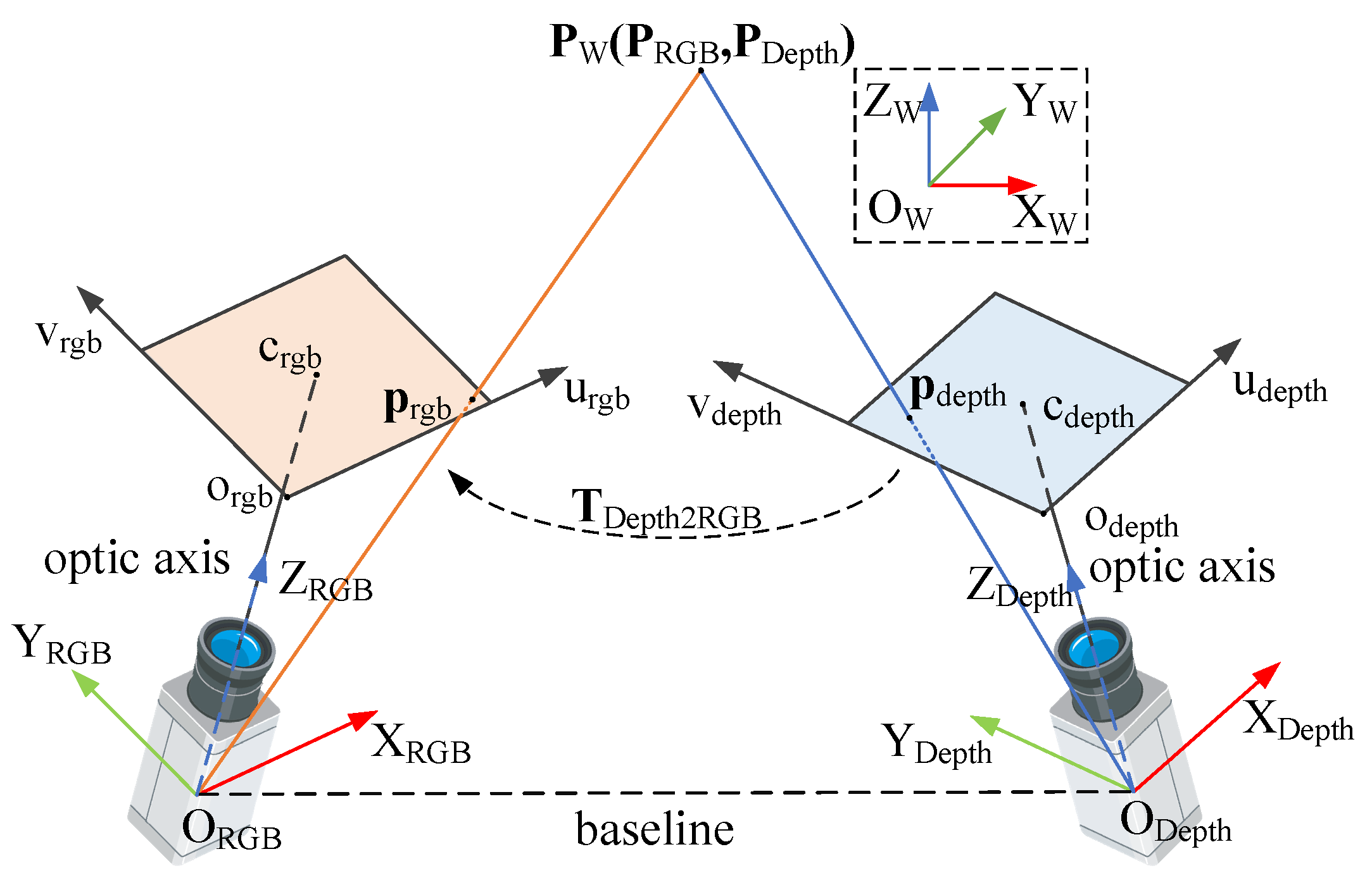
A schematic diagram of the RGB-D camera coordinate system is shown in Figure 2. It is assumed that the world coordinate system is ; the RGB camera coordinate system and the depth camera coordinate system are and , respectively; and the corresponding image pixel coordinate systems are and , respectively. The position of a world point, , in the RGB camera and the depth camera coordinate system are shown in the following formula.
The positional relationship between the RGB camera and the depth camera can be represented by the transformation matrix, , as follows:
The camera coordinate system can be converted to the camera image pixel coordinate system by the following equation.
where and represent the intrinsic parameter matrix of the RGB camera and the depth camera, respectively. By combining Equations (2) and (3), the depth image pixel coordinate system can be converted into the RGB image pixel coordinate system, as shown in the following equation.
where is the depth value measured by the depth camera, and , , and can be obtained by the Zhang camera calibration method [35]. Through Equation (4), we can obtain the projection of the depth data in the RGB image pixel coordinate system. However, because the depth image size is usually different from the RGB image size, the depth image size is generally kept consistent with the RGB image size through the sampling method in the RGB image pixel coordinate system.
3.2. Feature Extraction from RGB Maps
- (1)
- SIFT
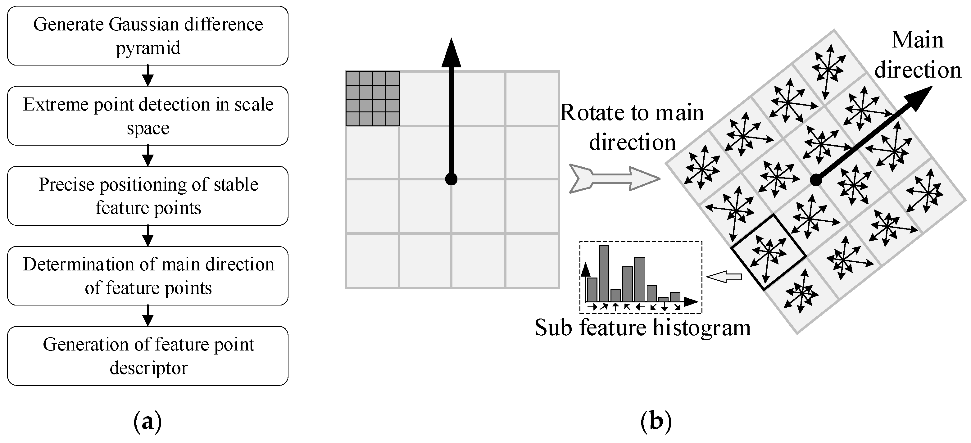
The process of SIFT feature point extraction and representation is shown in Figure 3a. After determining the location of the feature point, SIFT takes 4 × 4 subregion blocks around the feature point (each subregion block is 4 × 4 pixels), calculates the gradient amplitude and direction of each subregion, divides the gradient direction into eight intervals, and counts each subregion into an eight-dimensional subfeature histogram. The subfeature histograms of 4 × 4 subregion blocks are combined to form a 128-dimensional SIFT feature descriptor. A schematic diagram is shown in Figure 3b.
- (12)
- SURF
The process of SURF feature point extraction and representation is shown in Figure 4a. After determining the position of the feature point, SURF takes 4 × 4 subregion blocks around the feature point and rotates them to the main direction of the feature points. Each subregion counts the Haar wavelet features of 25 pixels in the horizontal and vertical directions to obtain the sum of horizontal values, the sum of vertical values, the sum of absolute horizontal values, and the sum of absolute vertical values. The four feature quantities of the 4 × 4 subregion blocks are then combined to form a 64-dimensional SURF feature descriptor. A schematic diagram is shown in Figure 4b.
- (3)
- ORB
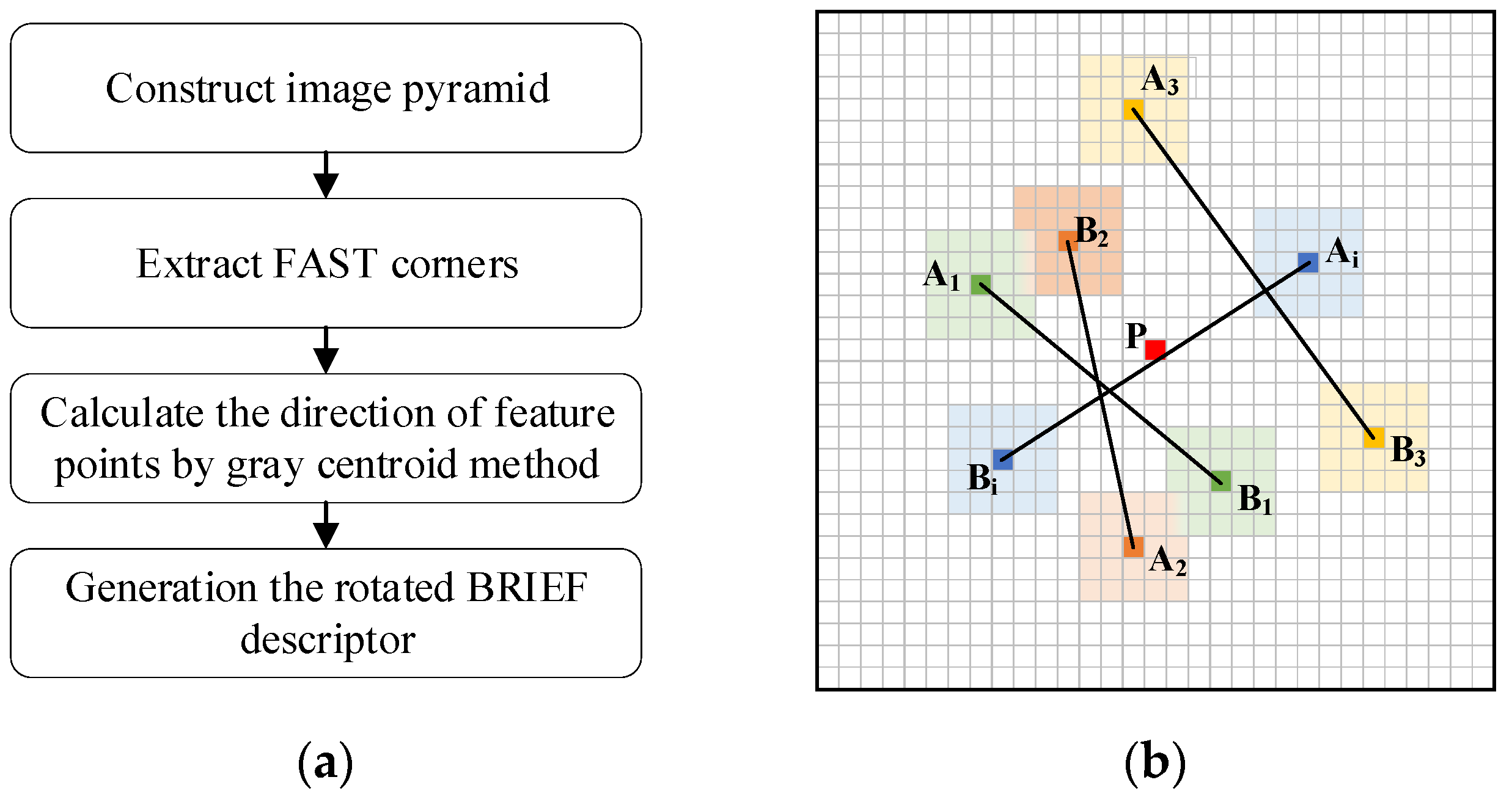
The process of ORB feature point extraction and representation is shown in Figure 5a. After determining the position of the feature point, ORB selects a 31 × 31 image block with the feature point as the center, rotates it to the main direction, and then randomly selects N pairs of points in this block (N is generally 128, 256, or 512). For point pairs A and B, a binary result is achieved by comparing the average size of the grayscale in the 5 × 5 subwindow around the two points and comparing N pairs of points to obtain a length N binary feature descriptor. A schematic diagram is shown in Figure 5b.
3.3. Feature Extraction from Point Cloud
- (1)
- PFH
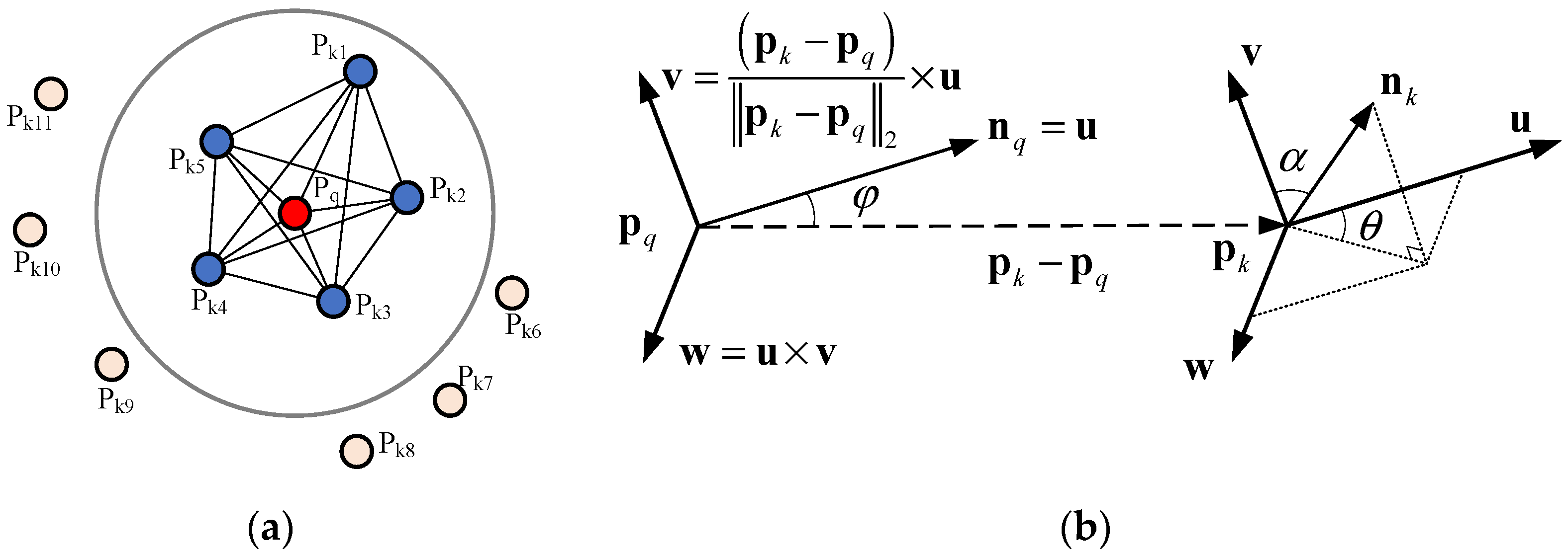
PFH parameterizes the spatial difference between a reference point and its neighborhood to form a multidimensional histogram describing the geometric properties of the point neighborhood. The multidimensional space where the histogram is located provides a measurable information space for feature expression and is robust to pose, sampling density, and noise of 3D surfaces. As shown in Figure 6a, represents the sampling point (red). The scope of PFH is a sphere with as the center and radius . Other points in the scope contribute to the PFH of (blue). After obtaining all the neighboring points in the k neighborhood of sampling point , a local coordinate system, , is established at Pq, as shown in Figure 6b, where represents a neighborhood point, and and represent the normal at and , respectively.
In Figure 6b, the angle eigenvalues of , , and are as follows.
Each angle eigenvalue is divided into five intervals. All adjacent points in the K neighborhood are combined in pairs to form a new point pair, and the times of , , and values of the point pair falling in each angle interval are counted. Finally, a 125-dimensional point feature histogram is obtained.
- (2)
- FPFH
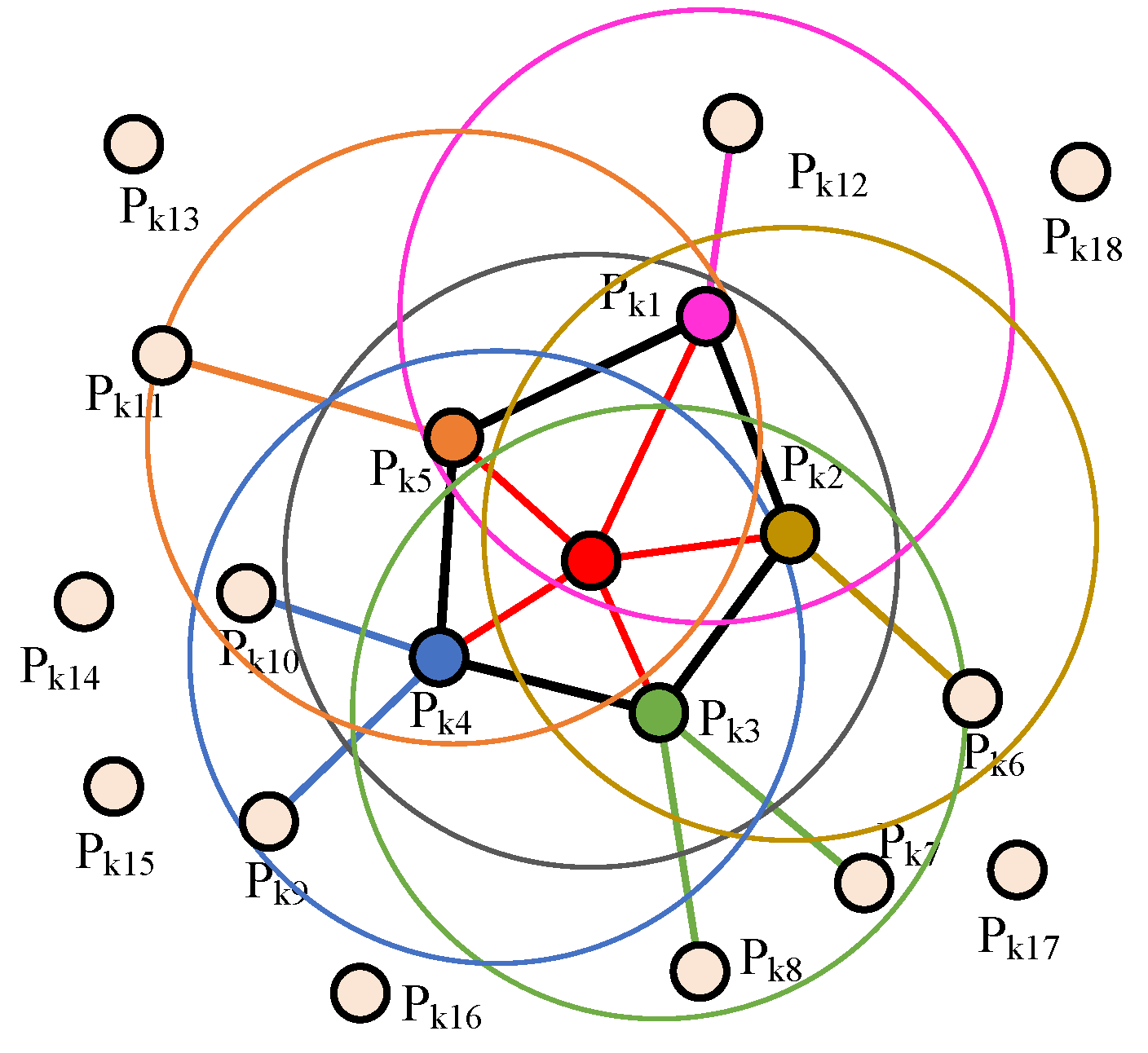
As a simplified algorithm of PFH, the FPFH algorithm maintains good robustness and recognition characteristics. It also improves the matching speed and achieves excellent real-time performance by simplifying and reducing the computational complexity. The specific calculation process of FPFH is as follows:
- For each sample point, the three angle eigenvalues are calculated between the point and each point in its K neighborhood, and each angle eigenvalue is divided into 11 intervals, so a 33-dimensional simplified point feature histogram (SPFH) is obtained;
- The K-neighborhood points of each point are calculated to form their SPFH;
- The final FPFH is calculated with the following formula:
A schematic diagram of the FPFH affected area is shown in Figure 7.
3.4. Feature Fusion
Due to the varying data types of different descriptors, we propose different descriptor fusion methods for different types of feature descriptors.
- (1)
- SIFT and SURF feature descriptors, as well as those of PFH and FPFH are floating-point descriptors. For this kind of floating-point feature descriptor, we propose direct splicing of the normalized point cloud feature descriptors after the normalized image feature descriptors to form the fusion feature descriptors SIFTPFH, SIFTFPFH, SURFPFH, and SURFFPFH.
- (2)
- The image feature descriptor of ORB is a binary string, and the point cloud feature descriptors of PFH and FPFH are floating-point descriptors. In order to maintain the respective feature-description ability of binary descriptors and floating-point descriptors, the data types of the two descriptors are kept unchanged and combined into a tuple, thereby obtaining the fusion feature descriptors of ORBPFH and ORBFPFH. Because the norm of PFH or FPFH is minor, to increase the weight of point cloud features, we usually multiply a coefficient to make the norm of PFH or FPFH after multiplication close to the length of ORB features.
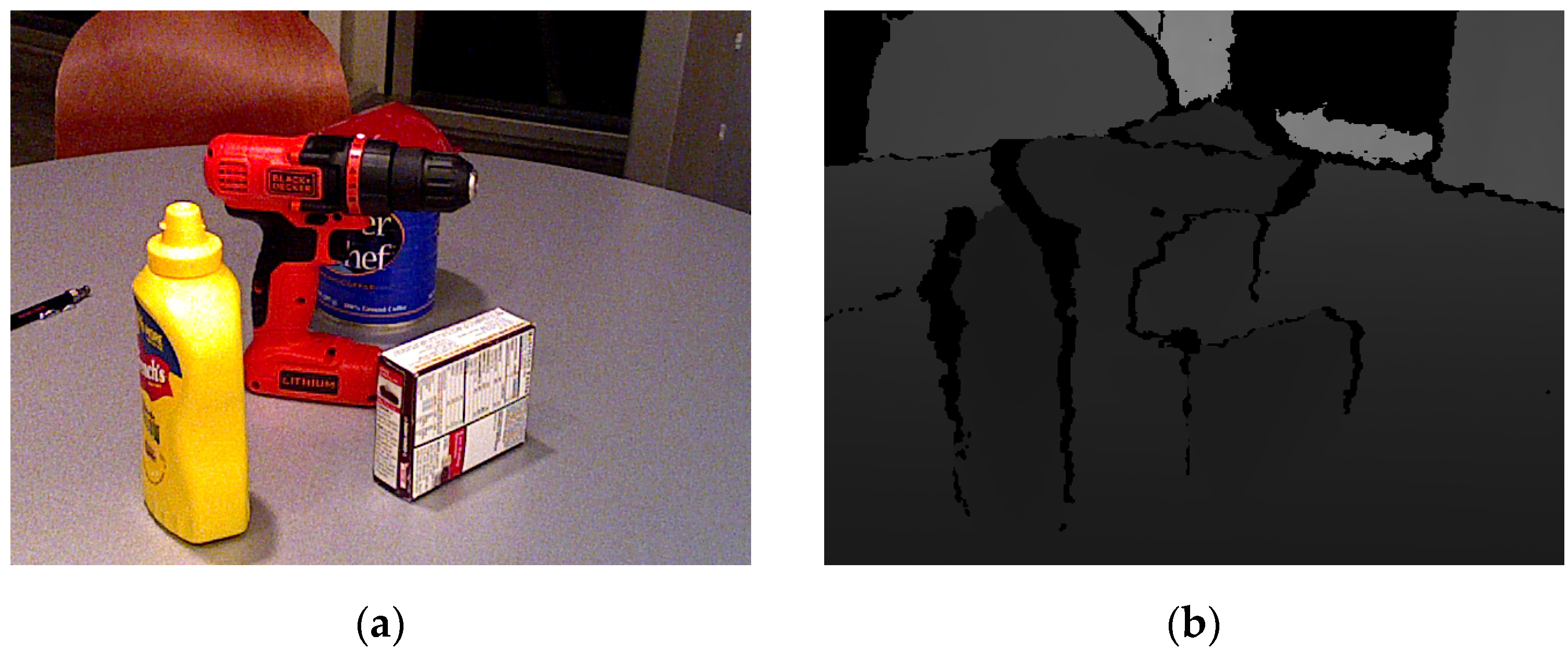
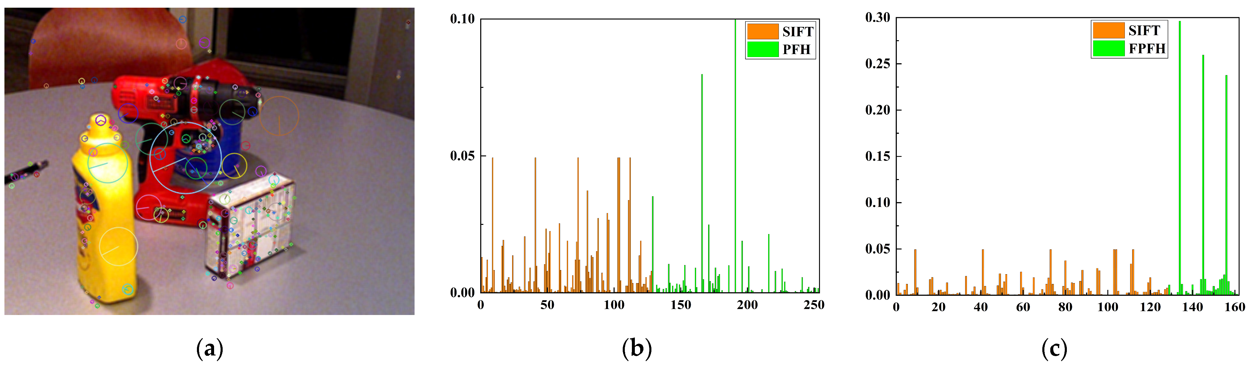
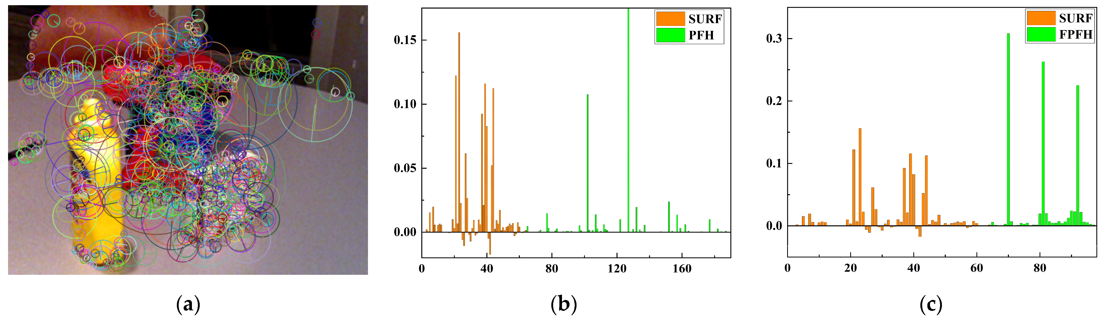
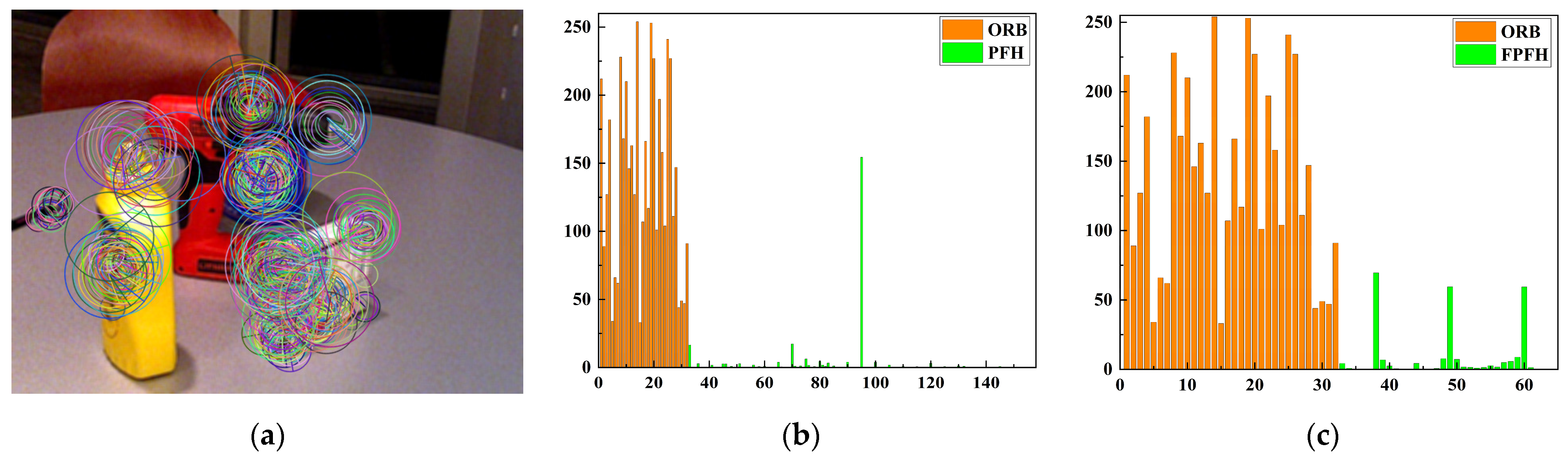
Figure 8 shows an RGB-D image in the Yale-CMU-Berkeley (YCB) dataset, and Figure 9, Figure 10 and Figure 11 show the feature points and different fusion feature histograms of the RGB-D image.
As can be seen from the above figures, the fusion of the two feature descriptors expands the descriptor’s length, enriches the descriptor information, strengthens the constraints of the descriptor, and makes it more special.
3.5. Feature Matching
The data types of the SIFTPFH, SIFTFPFH, SURFPFH, and SURFFPFH feature descriptors are floating point. Therefore, the Euclidean distance is used as the feature point similarity evaluation index, and the specific formula is as follows.
where and are the feature descriptors to be registered.
As mentioned earlier, the ORBPFH or ORBFPFH feature descriptor is a tuple in which the Hamming distance of the ORB descriptor is calculated, the Euclidean distance of the PFH or FPFH descriptor is calculated, and the two distances are added to obtain the final feature distance; the specific formula is as follows. The calculation process of the Hamming involves comparing whether each bit of the binary feature descriptor is the same. If not, add 1 to the Hamming distance.
where indicates whether the bit is the same, its definition is as follows, represents the length of the ORB feature descriptor, and represents the total length of the ORBPFH or ORBFPFH feature descriptor.
Then, the rough registration of the feature point is realized based on the Fast Library for Approximate Nearest Neighbors (FLANN) algorithm. Finally, the random sample consensus (RANSAC) algorithm is used to accurately register feature points.
4. Experiment and Results
The performance of the proposed feature extraction and fusion method is verified on the RGB-D datasets of YCB and Karlsruhe Institute of Technology and Toyota Technological Institute (KITTI). The specific index parameters characterizing the performance of the descriptor are the number and time of feature extraction, the number and time of feature matching, and the matching failure rate. The definition of the matching failure rate (MFR) is as follows.
where represents the number of matching failed frames, and represents the total number of frames.
The image resolution of the RGB-D image is 640 × 480. After the depth image is transformed into a point cloud, there are about 300,000 points. Such a colossal point cloud will consume many computing resources and time when calculating the normal vector and PFH/FPFH descriptor. Therefore, the point cloud is downsampled to keep the number of points in the range of 2000 to 5000, ensuring calculation accuracy and reducing the calculation time.
The sample image of the YCB dataset is shown in Figure 12, and its indices are shown in Table 1. A sample image of the KITTI dataset is shown in Figure 13, and its indices are shown in Table 2. In Table 1 and Table 2, Ne indicates the number of extracted feature points, Nm indicates the number of matched feature points, Te indicates the time of feature extraction, Tm indicates the time of feature matching, and Ta indicates the total time.
Table 1 and Table 2 show that the time of feature extraction and registration are ordered as follows: image features <image features + FPFH <image features + PFH. In particular, it is worth noting that the consumption time of ORBFPFH is less than that of SURF and SIFT, indicating that ORBFPFH has the potential to be applied in a real-time system.
Taking the first frame in the YCB 0024 dataset as a reference frame, the failure rates of feature matching between the first 200 frames, the first 280 frames, and the first 300 frames in the dataset and the reference frame is counted. The results are shown in Table 3. Taking the first frame in the KITTI fire dataset as the reference frame, the failure rates of feature matching between the first 100 frames, the first 125 frames, and the first 150 frames in the dataset and the reference frames are counted. The results are shown in Table 4. In Table 3 and Table 4, failed Nm indicates the number of failed matching frames. The matching results of different fusion features are available in the Supplementary Materials.
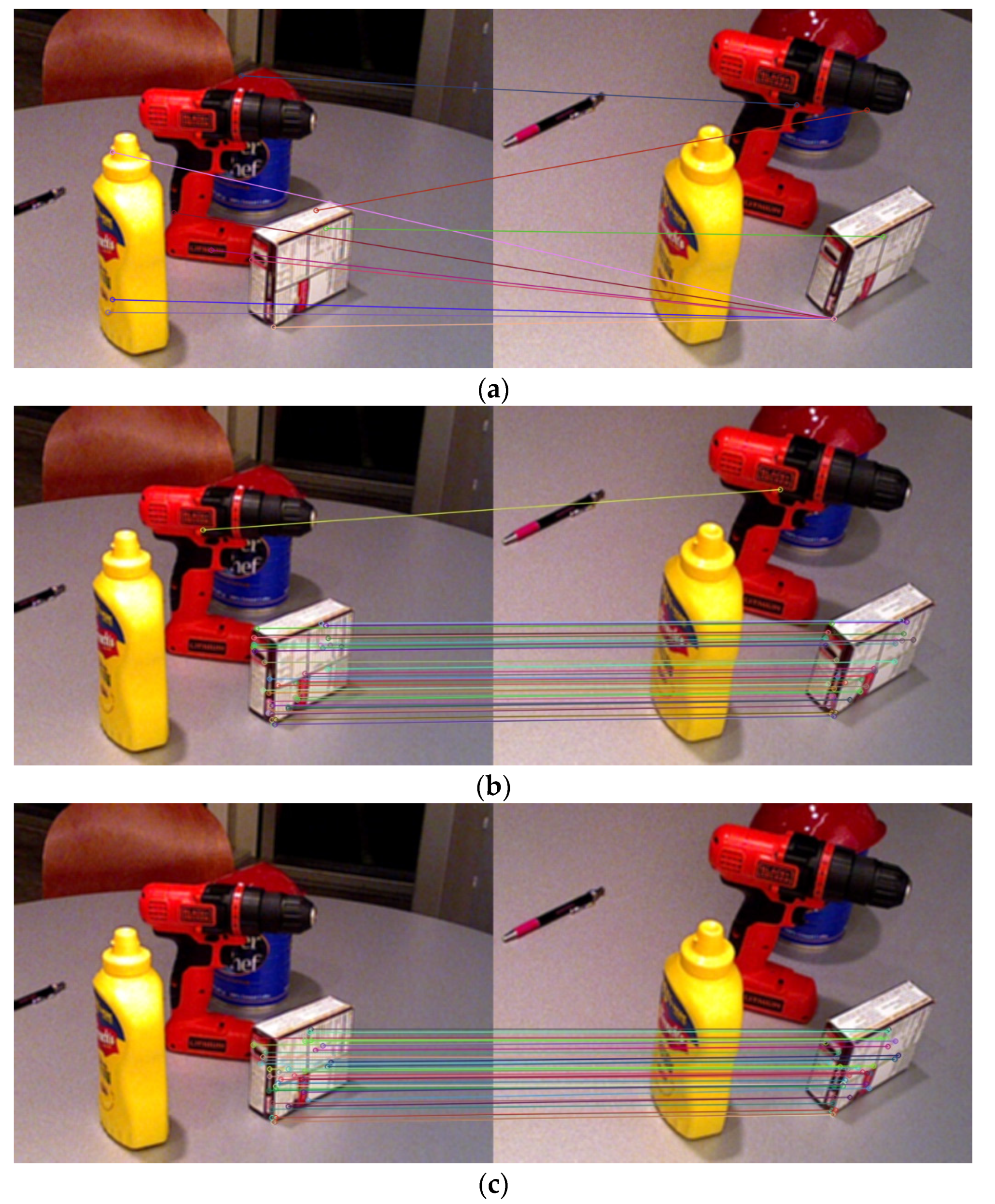
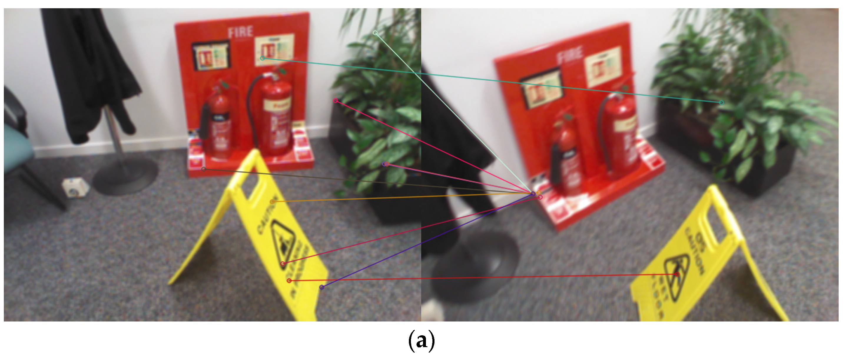
As shown in Table 3 and Table 4, the feature-matching failure rate of the fused feature descriptors SIFTPFH and SIFTFPFH is much higher than that of SIFT, indicating that point cloud feature descriptors PFH and FPFH reduce the feature representation ability of SIFT. The feature-matching failure rate of the fused feature descriptors SURFPFH and SURFFPFH is similar to that of SURF, indicating that the point cloud feature descriptors PFH and FPFH are not very helpful for improving the feature-representation ability of SURF. The feature-matching failure rates of the fusion feature descriptors ORBPFH and ORBFPFH are lower than those of ORB. On the test dataset, ORBPFH reduces the matching failure rate by 4.66~16.66% compared with ORB, and ORBFPFH reduces the false-matching rate by 9~20% compared with ORB, indicating that point cloud feature descriptors PFH and FPFH improve the feature-representation ability of orb descriptors. Some examples of successful registration of ORBPFH and ORBFPFH but failed registration of ORB are shown in Figure 14 and Figure 15.
The above results show that the feature extraction and fusion method proposed in this paper is suitable for fusing PFH and FPFH features with ORB features, offering a novel approach for RGB-D image matching.
5. Conclusions
To effectively fuse image and depth information and improve feature-matching accuracy of RGB-D images, a robust image feature extraction and fusion method based on image feature and depth information fusion is proposed in this paper. The proposed method directly splices the image feature point descriptor with the corresponding point cloud feature descriptor to obtain the fusion descriptor of feature points. The fusion feature descriptors are constructed according to the SIFT, SURF, and ORB image feature descriptor and the PFH and FPFH point cloud feature descriptor. The performance of the fusion features is tested in the RGB-D dataset of YCB and KITTI. On the test dataset, ORBPFH reduces the matching failure rate by 4.66~16.66%, ORBFPFH reduces the matching failure rate by 9~20%, and ORBFPFH has potential for real-time application. The test results show that the robust feature extraction and fusion method proposed in this paper is suitable for the fusion of ORB features with PFH and FPFH features and can improve the ability of feature representation and registration, representing a novel approach for RGB-D image matching.
Supplementary Materials
The following supporting information can be downloaded at: https://doi.org/10.6084/m9.figshare.19635075.v2, Figures: The matching results of different fusion features.
Author Contributions
Conceptualization, H.W.; methodology, Z.Y.; software, Z.Y.; validation, Z.Y., Q.N. and Y.L.; formal analysis, Z.Y.; investigation, Z.Y.; writing—original draft preparation, Z.Y.; writing—review and editing, Z.Y. and H.W.; visualization, Z.Y. and Q.N.; supervision, H.W.; project administration, H.W.; funding acquisition, H.W. All authors have read and agreed to the published version of the manuscript.
Funding
This research was funded by the National Natural Science Foundation of China, grant number 61705220.
Institutional Review Board Statement
Not applicable.
Informed Consent Statement
Not applicable.
Data Availability Statement
Not applicable.
Acknowledgments
The authors would like to acknowledge KITTI and YCB dataset for making their datasets available to us.
Conflicts of Interest
The authors declare no conflict of interest.
References
- Lowe, D.G. Object recognition from local scale-invariant features. In Proceedings of the Seventh IEEE International Conference on Computer Vision, Kerkyra, Greece, 20–27 September 1999; pp. 1150–1157. [Google Scholar]
- Rosten, E.; Drummond, T. Machine learning for high-speed corner detection. In Proceedings of the European Conference on Computer Vision, Graz, Austria, 7–13 May 2006; pp. 430–443. [Google Scholar]
- Bay, H.; Ess, A.; Tuytelaars, T.; Van Gool, L. Speeded-up robust features (SURF). Comput. Vis. Image Underst. 2008, 110, 346–359. [Google Scholar] [CrossRef]
- Leutenegger, S.; Chli, M.; Siegwart, R.Y. BRISK: Binary robust invariant scalable keypoints. In Proceedings of the 2011 International Conference on Computer Vision, Washington, DC, USA, 6–13 November 2011; pp. 2548–2555. [Google Scholar]
- Rublee, E.; Rabaud, V.; Konolige, K.; Bradski, G. ORB: An efficient alternative to SIFT or SURF. In Proceedings of the 2011 International Conference on Computer Vision, Washington, DC, USA, 6–13 November 2011; pp. 2564–2571. [Google Scholar]
- Calonder, M.; Lepetit, V.; Strecha, C.; Fua, P. Brief: Binary robust independent elementary features. In Proceedings of the European Conference on Computer Vision, Crete, Greece, 5–11 September 2010; pp. 778–792. [Google Scholar]
- Alahi, A.; Ortiz, R.; Vandergheynst, P. Freak: Fast retina keypoint. In Proceedings of the 2012 IEEE Conference on Computer Vision and Pattern Recognition, Washington, DC, USA, 16–21 June 2012; pp. 510–517. [Google Scholar]
- Johnson, A.E.; Hebert, M. Using spin images for efficient object recognition in cluttered 3D scenes. IEEE Trans. Pattern Anal. Mach. Intell. 1999, 21, 433–449. [Google Scholar] [CrossRef] [Green Version]
- Frome, A.; Huber, D.; Kolluri, R.; Bülow, T.; Malik, J. Recognizing objects in range data using regional point descriptors. In Proceedings of the European Conference on Computer Vision, Prague, Czech Republic, 11–14 May 2004; pp. 224–237. [Google Scholar]
- Belongie, S.; Malik, J.; Puzicha, J. Shape matching and object recognition using shape contexts. IEEE Trans. Pattern Anal. Mach. Intell. 2002, 24, 509–522. [Google Scholar] [CrossRef] [Green Version]
- Rusu, R.B.; Blodow, N.; Marton, Z.C.; Beetz, M. Aligning point cloud views using persistent feature histograms. In Proceedings of the 2008 IEEE/RSJ International Conference on Intelligent Robots and Systems, Nice, France, 22–26 September 2008; pp. 3384–3391. [Google Scholar]
- Rusu, R.B.; Marton, Z.C.; Blodow, N.; Beetz, M. Learning informative point classes for the acquisition of object model maps. In Proceedings of the 2008 10th International Conference on Control, Automation, Robotics and Vision, Hanoi, Vietnam, 17–20 December 2008; pp. 643–650. [Google Scholar]
- Rusu, R.B.; Blodow, N.; Beetz, M. Fast point feature histograms (FPFH) for 3D registration. In Proceedings of the 2009 IEEE International Conference on Robotics and Automation, Kobe, Japan, 12–17 May 2009; pp. 3212–3217. [Google Scholar]
- Tombari, F.; Salti, S.; Stefano, L.D. Unique signatures of histograms for local surface description. In Proceedings of the European Conference on Computer Vision, Crete, Greece, 5–11 September 2010; pp. 356–369. [Google Scholar]
- Salti, S.; Tombari, F.; Di Stefano, L. SHOT: Unique signatures of histograms for surface and texture description. Comput. Vis. Image Underst. 2014, 125, 251–264. [Google Scholar] [CrossRef]
- Steder, B.; Rusu, R.B.; Konolige, K.; Burgard, W. NARF: 3D range image features for object recognition. In Proceedings of the Workshop on Defining and Solving Realistic Perception Problems in Personal Robotics at the IEEE/RSJ International Conference on Intelligent Robots and Systems (IROS), Taibei, China, 18–22 October 2010. [Google Scholar]
- Guo, Y.; Sohel, F.; Bennamoun, M.; Lu, M.; Wan, J. Rotational projection statistics for 3D local surface description and object recognition. Int. J. Comput. Vis. 2013, 105, 63–86. [Google Scholar] [CrossRef] [Green Version]
- Prakhya, S.M.; Liu, B.; Lin, W. B-SHOT: A binary feature descriptor for fast and efficient keypoint matching on 3D point clouds. In Proceedings of the 2015 IEEE/RSJ International Conference on Intelligent Robots and Systems (IROS), Hamburg, Germany, 28 September–2 October 2015; pp. 1929–1934. [Google Scholar]
- Shen, Z.; Ma, X.; Zeng, X. Hybrid 3D surface description with global frames and local signatures of histograms. In Proceedings of the 2018 24th International Conference on Pattern Recognition (ICPR), Beijing, China, 20–24 August 2018; pp. 1610–1615. [Google Scholar]
- Yang, J.; Cao, Z.; Zhang, Q. A fast and robust local descriptor for 3D point cloud registration. Inf. Sci. 2016, 346, 163–179. [Google Scholar] [CrossRef]
- Srivastava, S.; Lall, B. 3D binary signatures. In Proceedings of the Tenth Indian Conference on Computer Vision, Graphics and Image Processing, Guwahati, India, 18–22 December 2016; pp. 1–8. [Google Scholar]
- Prakhya, S.M.; Lin, J.; Chandrasekhar, V.; Lin, W.; Liu, B. 3DHoPD: A fast low-dimensional 3-D descriptor. IEEE Robot. Autom. Lett. 2017, 2, 1472–1479. [Google Scholar] [CrossRef]
- Yang, J.; Zhang, Q.; Xiao, Y.; Cao, Z. TOLDI: An effective and robust approach for 3D local shape description. Pattern Recognit. 2017, 65, 175–187. [Google Scholar] [CrossRef]
- Rehman, S.U.; Asad, H. A novel approach for feature extraction from RGB-D data. Technology 2017, 3, 1538–1541. [Google Scholar]
- Zou, Y.; Wang, X.; Zhang, T.; Liang, B.; Song, J.; Liu, H. BRoPH: An efficient and compact binary descriptor for 3D point clouds. Pattern Recognit. 2018, 76, 522–536. [Google Scholar] [CrossRef]
- Quan, S.; Ma, J.; Hu, F.; Fang, B.; Ma, T. Local voxelized structure for 3D binary feature representation and robust registration of point clouds from low-cost sensors. Inf. Sci. 2018, 444, 153–171. [Google Scholar]
- Khan, W.; Phaisangittisagul, E.; Ali, L.; Gansawat, D.; Kumazawa, I. Combining features for RGB-D object recognition. In Proceedings of the 2017 International Electrical Engineering Congress (iEECON), Pattaya, Thailand, 8–10 March 2017; pp. 1–5. [Google Scholar]
- Alshawabkeh, Y. Linear feature extraction from point cloud using color information. Herit. Sci. 2020, 8, 28. [Google Scholar] [CrossRef]
- Chen, H.; Sun, D. Feature extraction of point cloud using 2D-3D transformation. In Proceedings of the Twelfth International Conference on Graphics and Image Processing (ICGIP 2020), Xi’an, China, 13–15 November 2021; p. 117200P. [Google Scholar]
- Li, Y.; Luo, Y.; Gu, X.; Chen, D.; Gao, F.; Shuang, F. Point cloud classification algorithm based on the fusion of the local binary pattern features and structural features of voxels. Remote Sens. 2021, 13, 3156. [Google Scholar] [CrossRef]
- Pan, L.; Zhou, X.; Shi, R.; Zhang, J.; Yan, C. Cross-modal feature extraction and integration based RGBD saliency detection. Image Vis. Comput. 2020, 101, 103964. [Google Scholar] [CrossRef]
- Tian, J.; Cheng, W.; Sun, Y.; Li, G.; Jiang, D.; Jiang, G.; Tao, B.; Zhao, H.; Chen, D. Gesture recognition based on multilevel multimodal feature fusion. J. Intell. Fuzzy Syst. 2020, 38, 2539–2550. [Google Scholar] [CrossRef]
- Zhu, X.; Li, Y.; Fu, H.; Fan, X.; Shi, Y.; Lei, J. RGB-D salient object detection via cross-modal joint feature extraction and low-bound fusion loss. Neurocomputing 2021, 453, 623–635. [Google Scholar] [CrossRef]
- Bai, J.; Wu, Y.; Zhang, J.; Chen, F. Subset based deep learning for RGB-D object recognition. Neurocomputing 2015, 165, 280–292. [Google Scholar] [CrossRef]
- Zhang, Z. Flexible camera calibration by viewing a plane from unknown orientations. In Proceedings of the the Seventh IEEE International Conference on Computer Vision, Kerkyra, Greece, 20–27 September 1999; pp. 666–673. [Google Scholar]
Figure 1.
Sample graph with blue (dotted), green (solid), and red (dashed) lines.

Figure 2.
The schematic diagram of the RGB-D coordinate system.

Figure 3.
Feature point extraction and representation of SIFT. (a) SIFT feature point extraction and representation process; (b) SIFT descriptor generation process.
Figure 3.
Feature point extraction and representation of SIFT. (a) SIFT feature point extraction and representation process; (b) SIFT descriptor generation process.

Figure 4.
Feature point extraction and representation of SURF. (a) SURF feature point extraction and representation process; (b) SURF descriptor generation process.
Figure 4.
Feature point extraction and representation of SURF. (a) SURF feature point extraction and representation process; (b) SURF descriptor generation process.

Figure 5.
Feature point extraction and representation of ORB. (a) ORB feature point extraction and representation process; (b) schematic diagram of the rotated BRIEF descriptor generation.
Figure 5.
Feature point extraction and representation of ORB. (a) ORB feature point extraction and representation process; (b) schematic diagram of the rotated BRIEF descriptor generation.

Figure 6.
Feature point extraction and representation of ORB. (a) Schematic diagram of PFH, and , ..., represent points around the sampling point ; (b) schematic diagram of PFH coordinate system.
Figure 6.
Feature point extraction and representation of ORB. (a) Schematic diagram of PFH, and , ..., represent points around the sampling point ; (b) schematic diagram of PFH coordinate system.

Figure 7.
Schematic diagram of the affected area of FPFH.

Figure 8.
An example of an RGB-D image in the YCB dataset. (a) RGB image; (b) depth image.

Figure 9.
Extracted SIFT feature points and feature histograms of SIFTPFH and SIFTFPFH at pixel (374, 373). (a) Extracted SIFT feature points; (b) SIFTPFH feature histogram; (c) SIFTFPFH feature histogram.
Figure 9.
Extracted SIFT feature points and feature histograms of SIFTPFH and SIFTFPFH at pixel (374, 373). (a) Extracted SIFT feature points; (b) SIFTPFH feature histogram; (c) SIFTFPFH feature histogram.

Figure 10.
Extracted SURF feature points and feature histograms of SURFPFH and SURFFPFH at pixel (374, 373). (a) Extracted SURF feature points; (b) SURFPFH feature histogram; (c) SURFFPFH feature histogram.
Figure 10.
Extracted SURF feature points and feature histograms of SURFPFH and SURFFPFH at pixel (374, 373). (a) Extracted SURF feature points; (b) SURFPFH feature histogram; (c) SURFFPFH feature histogram.

Figure 11.
Extracted ORB feature points and feature histograms of ORBPFH and ORBFPFH at pixel (374, 373); the norm of PFH or FPFH here is 256. (a) Extracted ORB feature points; (b) ORBPFH feature histogram; (c) ORBFPFH feature histogram.
Figure 11.
Extracted ORB feature points and feature histograms of ORBPFH and ORBFPFH at pixel (374, 373); the norm of PFH or FPFH here is 256. (a) Extracted ORB feature points; (b) ORBPFH feature histogram; (c) ORBFPFH feature histogram.

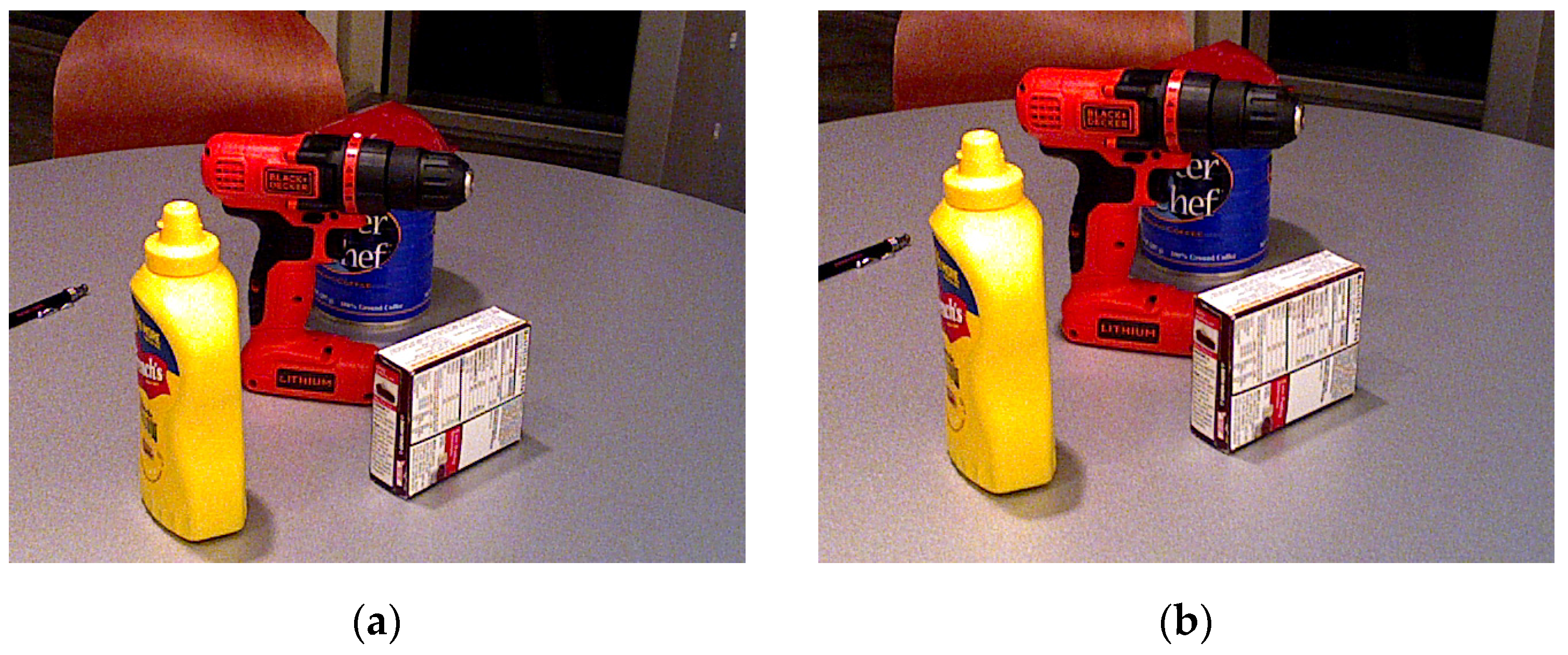
Figure 12.
Test images in the YCB 0024 dataset. (a) 000001-color; (b) 000050-color.

Figure 13.
Test images in the KITTI fire dataset. (a) frame-000001.color; (b) frame-000050.color.

Figure 14.
Example of successful registration of ORBPFH and ORBFPFH but failed registration of ORB. (a) ORB registration of frames 1 and 227 in the YCB 0024 dataset. (b) ORBPFH registration of frames 1 and 227 in the YCB 0024 dataset. (c) ORBFPFH registration of frames 1 and 227 in the YCB 0024 dataset.

Figure 15.
Examples of successful registration of ORBPFH and ORBFPFH but failed registration of ORB. (a) ORB registration of frames 1 and 92 in the KITTI fire dataset. (b) ORBPFH registration of frames 1 and 92 in the KITTI fire dataset. (c) ORBFPFH registration of frames 1 and 92 in the KITTI fire dataset.


Table 1.
Test results of the YCB 0024 dataset.
| Descriptor | Ne | Nm | Te (ms) | Tm (ms) | Ta (ms) | |
|---|---|---|---|---|---|---|
| 1st Img | 2nd Img | |||||
| SIFT | 400 | 400 | 129 | 309 | 19 | 328 |
| SIFTPFH | 400 | 400 | 111 | 848 | 19 | 867 |
| SIFTFPFH | 400 | 400 | 117 | 418 | 15 | 433 |
| SURF | 961 | 991 | 245 | 286 | 31 | 317 |
| SURFPFH | 961 | 991 | 182 | 2425 | 49 | 2474 |
| SURFFPFH | 961 | 991 | 199 | 523 | 31 | 554 |
| ORB | 421 | 433 | 103 | 2 | 11 | 13 |
| ORBPFH | 421 | 433 | 160 | 698 | 9 | 707 |
| ORBFPFH | 421 | 433 | 145 | 108 | 9 | 117 |
Table 2.
Test results of the KITTI fire dataset.
| Descriptor | Ne | Nm | Te (ms) | Tm (ms) | Ta (ms) | |
|---|---|---|---|---|---|---|
| 1st Img | 2nd Img | |||||
| SIFT | 400 | 321 | 37 | 309 | 34 | 343 |
| SIFTPFH | 400 | 321 | 26 | 741 | 34 | 775 |
| SIFTFPFH | 400 | 321 | 32 | 433 | 34 | 467 |
| SURF | 1347 | 1169 | 51 | 286 | 49 | 335 |
| SURFPFH | 1347 | 1169 | 29 | 2726 | 65 | 2791 |
| SURFFPFH | 1347 | 1169 | 40 | 562 | 49 | 611 |
| ORB | 347 | 220 | 47 | 2 | 28 | 30 |
| ORBPFH | 347 | 220 | 36 | 378 | 26 | 404 |
| ORBFPFH | 347 | 220 | 38 | 88 | 25 | 113 |
Table 3.
Failure rate of feature matching in the YCB 0024 dataset.
| Descriptor | Failed Nm | MFR | ||||
|---|---|---|---|---|---|---|
| Total frames | 200 | 280 | 300 | 200 | 280 | 300 |
| SIFT | 0 | 0 | 1 | 0% | 0% | 0.33% |
| SIFTPFH | 0 | 3 | 11 | 0% | 1.07% | 3.67% |
| SIFTFPFH | 2 | 20 | 32 | 1% | 7.14% | 10.67% |
| SURF | 0 | 29 | 45 | 0% | 10.36% | 15% |
| SURFPFH | 0 | 25 | 40 | 0% | 8.93% | 13.33% |
| SURFFPFH | 0 | 36 | 53 | 0% | 12.86% | 17.67% |
| ORB | 0 | 36 | 51 | 0% | 12.86% | 17% |
| ORBPFH | 0 | 0 | 1 | 0% | 0% | 0.33% |
| ORBFPFH | 0 | 0 | 0 | 0% | 0% | 0% |
Table 4.
Failure rate of feature matching in the KITTI fire dataset.
| Descriptor | Failed Nm | MFR | ||||
|---|---|---|---|---|---|---|
| Total frames | 100 | 125 | 150 | 100 | 125 | 150 |
| SIFT | 1 | 10 | 24 | 1% | 8% | 16% |
| SIFTPFH | 8 | 32 | 57 | 8% | 25.60% | 38% |
| SIFTFPFH | 6 | 23 | 48 | 6% | 18.40% | 32% |
| SURF | 16 | 41 | 66 | 16% | 32.80% | 44% |
| SURFPFH | 19 | 44 | 69 | 19% | 35.20% | 46% |
| SURFFPFH | 23 | 48 | 73 | 23% | 38.40% | 48.67% |
| ORB | 11 | 36 | 53 | 11% | 28.80% | 35.33% |
| ORBPFH | 4 | 26 | 46 | 4% | 20.80% | 30.67% |
| ORBFPFH | 2 | 19 | 23 | 2% | 15.20% | 15.33% |
Publisher’s Note: MDPI stays neutral with regard to jurisdictional claims in published maps and institutional affiliations. |
© 2022 by the authors. Licensee MDPI, Basel, Switzerland. This article is an open access article distributed under the terms and conditions of the Creative Commons Attribution (CC BY) license (https://creativecommons.org/licenses/by/4.0/).
Share and Cite
MDPI and ACS Style
Yan, Z.; Wang, H.; Ning, Q.; Lu, Y. Robust Image Matching Based on Image Feature and Depth Information Fusion. Machines 2022, 10, 456. https://doi.org/10.3390/machines10060456
AMA Style
Yan Z, Wang H, Ning Q, Lu Y. Robust Image Matching Based on Image Feature and Depth Information Fusion. Machines. 2022; 10(6):456. https://doi.org/10.3390/machines10060456
Chicago/Turabian StyleYan, Zhiqiang, Hongyuan Wang, Qianhao Ning, and Yinxi Lu. 2022. "Robust Image Matching Based on Image Feature and Depth Information Fusion" Machines 10, no. 6: 456. https://doi.org/10.3390/machines10060456
Note that from the first issue of 2016, this journal uses article numbers instead of page numbers. See further details here.