Morphological Component Analysis-Based Hidden Markov Model for Few-Shot Reliability Assessment of Bearing

Abstract

Reliability is of great significance in ensuring the safe operation of modern industry, which mainly relies on data analysis and life tests. However, as the life of mechanical systems becomes increasingly longer with the rapid development of the manufacturing industry, the collection of historical failure data becomes progressively more time-consuming. In this paper, a few-shot reliability assessment approach is proposed in order to overcome the dependence on historical data. Firstly, the vibration response of a bearing was illustrated. Then, based on a vibration response analysis, a morphological component analysis (MCA) method based on sparse representation theory was used to decompose vibration signals and extract impulse signals. After the impulse components’ reconstruction, their statistical indexes were utilized as the input observation vector of a Mixture of Gaussians Hidden Markov Model (MoG-HMM) for a reliability estimation. Finally, the experimental dataset of an aerospace bearing was analyzed via the proposed method. The comparison results illustrate the effectiveness of the proposed method of a few-shot reliability assessment.

1. Introduction

Reliability assessment is a critical consideration with regard to the proactive maintenance of equipment [1], which refers to the capability of a system or component to execute its essential functions under stated conditions in a given period of time. Statistics and mass production are enablers in the birth of reliability engineering.

Compared to reliability, the literature regarding operational reliability is much smaller. Abaei et al. proposed a systematic approach to evaluate the reliability of an autonomous system under the influence of uncertain disruptions, and to predict failure rates of unattended machinery plants [2]. Varshney et al. presented a performance analysis-based reliability estimation of a self-excited induction generator (SEIG) using the Monte-Carlo simulation (MCS) method, with data obtained from a self-excited induction motor operating as a generator [3]. Norouzi proposed a Pahlev reliability index for the resilience of power generation technologies versus climate change [4]. Cai used a proportional covariate model to construct the relationship between operation reliability and condition monitoring information [5]. Hu et al. introduced a decision-dependent uncertainty (DDU) in an operational reliability evaluation and proposed a power system operational reliability evaluation method [6]. Chai et al. proposed an operational reliability assessment method for photovoltaic inverters with considerations of voltage/VAR control functions [7], which can quantify reliability degradation and estimate the lifetime of PV inverters.

From the above literature and methods, it can be summarized that operational reliability methods mainly focus on feature extraction and mapping features to the reliability space. Deep learning provides an effective way to automatically extract features, which relies on a large number of training samples.

However, with the increase in mechanical component quality and service time, it becomes increasingly difficult and more time-consuming to obtain enough historical failure data. Therefore, the development of intelligent models with the ability of few-shot learning is urgent. Ren et al. proposed a capsule auto-encoder model that can extract vector features and achieve good results with few-shot samples [8]. Hu et al. proposed a task-sequencing meta-learning method to address the few-shot fault diagnosis problem. The experiment results illustrate that the proposed method can identify new categories with few samples [9]. Chen et al. proposed a hierarchy-guided transfer learning framework for few-shot fault recognition, which can learn a hierarchical structure of classes by multi-granularity clustering and by filtering out irrelevant categories, overcoming the problem of negative transfer [10]. In this paper, a few-shot reliability assessment method for a bearing is proposed, which shows a robust diagnosis performance with limited data, and is capable of working well under complex working conditions. In this method, the oscillation mechanism of a rotating mechanical system is first analyzed and discussed. Because both the vibration impact and the harmonic component will change with the variation of system condition according to the analysis, the system condition can be reflected by these sensitive fault components. Therefore, a morphological component analysis (MCA) approach based on a dual dictionary is used to extract the sensitive fault components as features. Meanwhile, it also mitigates the effect of noise. After separation and reconstruction, different signal components can be extracted from the original signals. Then, several classical statistical indexes of the impulse component are used as the input observation sequence O for MoG-HMM. This step includes two phases: the off-line phase, in which some initial normal condition signals are used to estimate the model λ of a corresponding MoG-HMM, and on-line phase, which continuously assesses the current health state of the physical component and estimate the maximum likelihood probability. Figure 1 shows a schematic sketch of the computational framework.

The remaining sections of this paper are organized as follows: Section 2 illustrates the vibration response of bearing and the proposed few-shot reliability assessment method; Section 3 presents the case studies; and discussions and conclusions are drawn in Section 4.

2. Methodology

When a signal contains components with distinct properties, its components can be separated via conventional LTI filters. However, in engineering practice, LTI filters often fail to apply because the harmonic component and impulse component are not separated in frequency. Sparse representation is a useful tool for solving this problem [11], and the use of sparsity to separate components of a signal is called morphological component analysis (MCA). MCA is an effective algorithm that has been widely used in the image processing field to separate smooth and textured components.

Therefore, a novel few-shot reliability assessment methodology is proposed in this study. This approach consists of two procedures: sparse components separation and few-shot reliability assessment.

2.1. Vibration Response of Bearing

Rotational machines are widely used in the manufacturing industry, and many mechanical structures can be simplified into a bearing–rotor system. The key component of rotational machines is a roller bearing–rotor system, which includes a rotational rotor and several roller bearings. Localized defects, such as cracks and spalls, may be generated during operations. When rolling elements roll over defects, shock pulses with short duration are generated, and excessive vibration may lead to a failure of the whole system [12].

In order to predict the dynamic behavior and vibration responses of a whole bearing–rotor system, dynamic modeling of the system is necessary. In this section, the dynamic model and vibration analysis are briefly described to accomplish the methodology [13].

When external forces are applied on the bearing, the distance between the curvature centers of raceway will be changed. $\mathrm{\Delta }{\delta }_x$, $\mathrm{\Delta }{\delta }_y$, $\mathrm{\Delta }{\delta }_z$, $\mathrm{\Delta }{\gamma }_y$ and $\mathrm{\Delta }{\gamma }_z$ are defined as the relative displacements of the five degrees of freedom in the inner raceway and outer raceway, respectively.

After the appearing deformation of the bearing, the distances between the ball center and the curvature center of inner and outer raceway are [13]:

$$\begin{array}{l}{\mathrm{\Delta }}_{ik}=r_i-\frac{D}{2}+{\delta }_{ik}=\left(f_i-0.5\right)D+{\delta }_{ik}\\ {\mathrm{\Delta }}_{ok}=r_o-\frac{D}{2}+{\delta }_{ok}=\left(f_o-0.5\right)D+{\delta }_{ok}\end{array}\}$$

(1)

where r_i and r_o are the curve radius of the inner and outer raceways, D is the diameter of balls, f_i and f_o are the ratios of the radius of the inner and outer raceways to the ball diameter, δ_ik and δ_ok are the contact deformation displacements of the ball at the inner and outer raceways, respectively. Then, displacement equations of geometric relations can be obtained [13]:

$$\begin{array}{c}{\left(U_{ik}-U_k\right)}^2+{\left(V_{ik}-V_k\right)}^2-{{\mathrm{\Delta }}_{ik}}^2=0\\ {U_k}^2+{V_k}^2-{{\mathrm{\Delta }}_{ok}}^2=0\end{array}\}$$

(2)

and the equilibrium equations for the ball can be given [10]:

$$\begin{array}{c}{Q}_{ik}\sin {\theta }_{ik}-Q_{ok}\sin {\theta }_{ok }-\frac{M_{gk}}{D}\left({\lambda }_{ik}\cos {\theta }_{ik}-{\lambda }_{ok}\cos {\theta }_{ok}\right)=0\\ Q_{ik}\cos {\theta }_{ik}-Q_{ok}\cos {\theta }_{ok}-\frac{M_{gk}}{D}\left({\lambda }_{ik}\sin {\theta }_{ik}-{\lambda }_{ok}\cos {\theta }_{ok}\right)+F_{ck}=0\end{array}\}$$

(3)

where Q_ik and Q_ok are the contact forces between the ball and the raceways, M_gk is the gyroscopic moment, θ_ik and θ_ok are the contact angles of the inner and outer raceways, and F_ck is the centrifugal force. Let λ_ik = λ_ok = 1. By Newton–Raphson method, Equations (2) and (3) and the force equilibrium equation can be solved, and U_ik, U_k, V_ik, V_k, Δ_ok, and Δ_ik can be obtained. Then, by adding all the forces between balls and the inner or outer raceways, the total force vector F_i (acting on the inner raceway) and F_o (acting on the outer raceway) can be obtained.

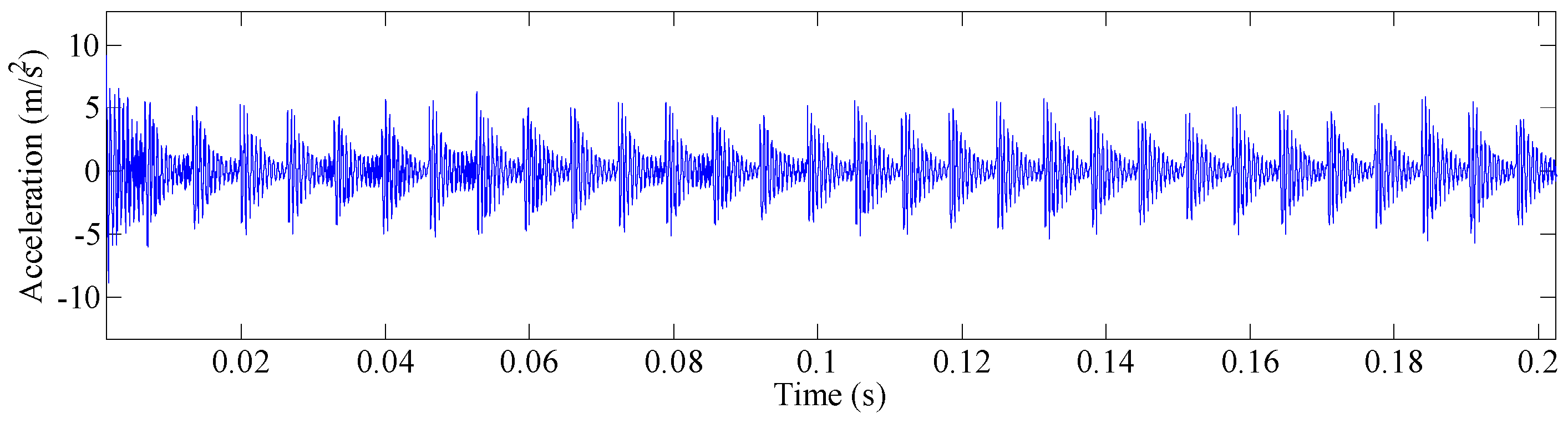
When the ball rolls in the raceway defect, the values of Δ_ok and Δ_ik will change, which will lead to change of the vibration response. When the ball comes into contact with the defect on the outer raceway, Δ_ok and Δ_ik become [13]:

$$\begin{array}{c}{\mathrm{\Delta }}_{ik}=r_i-\frac{D}{2}+{\delta }_{ik}=\left(f_i-0.5\right)D+{\delta }_{ik}\\ {\mathrm{\Delta }}_{ok}=r_o-\frac{D}{2}+{\delta }_{ok}=\left(f_o-0.5\right)D+{\delta }_{ok}+{\mathrm{\Delta }}_{so}\end{array}$$

(4)

where Δ_so is the additional deflection caused by an outer raceway defect. The acceleration response of the spindle nose in y direction is shown in Figure 2.

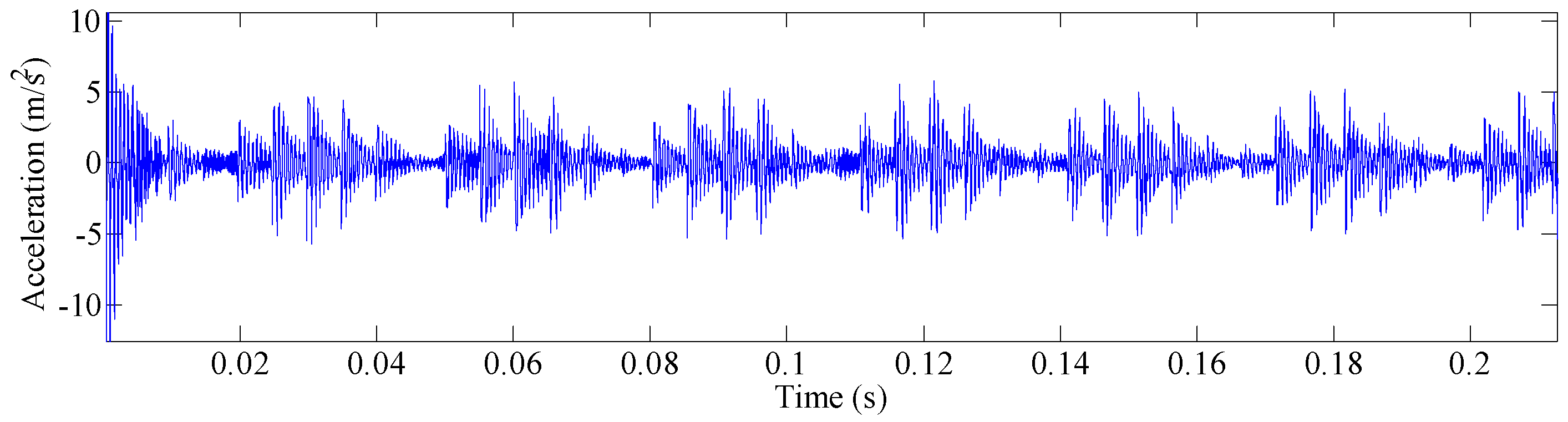
In the same way, the acceleration response of the spindle nose in y direction when the defect is located on the inner raceway is shown in Figure 3.

2.2. Sparse Components Separation Based on Dual-Basis Pursuit (Dual-BP)

Both the impulse and harmonic vibration increase with the operational time increase. In order to assess the few-shot reliability of a bearing–rotor system, these two components should be separated from the whole vibration signals. An MCA method based on BPDN [14] is applied in this study, which shows advantages in vibration information presentation and components separation, including super resolution, sparsity and noise reduction.

First of all, we used the l₁ and l₂ norms, which are defined as:

$$\begin{array}{l}{\Vert x\Vert }_1={\displaystyle \sum _{n=0}^{N-1}\left|x\left(n\right)\right|}\\ {\Vert x\Vert }_2^2={\displaystyle \sum _{n=0}^{N-1}{\left|x\left(n\right)\right|}^2}\end{array}$$

(5)

where N represents the length of x(n).

A discrete signal s(n) can be represented as:

$$s\left(n\right)=Ax\left(n\right)$$

(6)

where s(n) is an N-length vector. A is an over-complete dictionary, which is an N × M redundant matrix. x(n) is the sparse coefficient sequence, which is an M-length vector. For vibration signal of the bearing, A can be chosen as Fourier basis. To solve x(n), l₁-norm regularizer was used here [15]:

$$\begin{array}{l}\underset{x}{\arg \min }{\Vert x\Vert }_1\\ such that s=Ax\end{array}$$

(7)

When s is noisy, Equation (7) can be solved by minimizing the cost function, which is called the basis pursuit denoising (BPDN) problem:

$$\underset{x}{\arg \min }{\Vert s-Ax\Vert }_2^2+\lambda {\Vert x\Vert }_1$$

(8)

When a signal contains several components with distinct properties, two components in this application, the observed signal s(n) can be written as:

$$s\left(n\right)=s_1\left(n\right)+s_2\left(n\right)$$

(9)

If s₁(n) and s₂(n) are in distinct frequency bands, they can be separated using conventional LTI filters. However, in real signals collected from mechanical system, different components are never separated by frequency or other variables. Therefore, it is more challenging to separate these components. According to the morphological component analysis (MCA) method [16,17], it is assumed that each of the two components is best described using distinct transforms A₁ and A₂. As in Equation (6), s₁(n) and s₂(n) can be written as:

$$s_1=A_1{x}_1, s_2=A_2{x}_2$$

(10)

Therefore, to solve Equation (9), the MCA method is to find x₁ and x₂ such that:

$$s=A_1{x}_1+A_2{x}_2$$

(11)

which leads to the dual-basis pursuit (Dual-BP) problem:

$$\begin{array}{l}\underset{x_1,x_2}{\arg \min }{\lambda }_1{\Vert x_1\Vert }_1+{\lambda }_2{\Vert x_2\Vert }_1\\ such that s=A_1{x}_1+A_2{x}_2\end{array}$$

(12)

If s(n) is noisy, which is bound to occur in the actual vibration signals, Dual-BP problem turns into an MCA optimization problem:

$$\underset{x_1,x_2}{\arg \min }{\Vert s-A_1{x}_1-A_2{x}_2\Vert }_2^2+{\lambda }_1{\Vert x_1\Vert }_1+{\lambda }_2{\Vert x_2\Vert }_1$$

(13)

Parameters λ₁ and λ₁₂ should be chosen depending on the operating condition, which are usually set between 0 and 1. As λ₁ becomes larger, x₁ gains more weight. This paper employs the discrete Fourier basis and short-time Fourier basis as A₁ and A₂ because discrete Fourier basis can obtain a highly sparse representation of harmonic component, and short-time Fourier basis is suitable for sparse impact component representation.

Several algorithms are applicable for solving BP problem, such as iterative shrinkage/thresholding algorithm (ISTA) [18], block coordinate relaxation method [19], split variable augmented Lagrangian shrinkage algorithm (SALSA) [14], etc. SALSA is used to solve the MCA problem in this study.

Using the coefficients x₁ and x₂, the two components s₁ and s₂ can be obtained by Equation (10), and the impulse and harmonic components can be separated from the whole signal with proper parameters and basis. Because abrasion will take a long time to become faulty and cannot immediately lead to system damage, harmonic components are not as important as impulse components for reliability estimations. Then, several statistical indexes are utilized as the input observation sequence O for a Mixture of Gaussians Hidden Markov Model (MoG-HMM).

2.3. Few-Shot Reliability Assessment via Mixture of Gaussian Hidden Markov Models (MoG-HMM)

HMM is a stochastic technique for modeling signals that evolves through a finite number of states. The states are assumed to be hidden, and responsible for producing observations [20,21]. A basic HMM can be defined by three parameters: the transition probability matrix A, the observation model B, and initial state probability distribution π. Therefore, an HMM λ can be notated by λ = (A, B, π). Define S = (S₁, S₂, …, S_T) as the hidden state sequence and O = (O₁, O₂, …, O_T) as the observation sequence.

HMMs are usually used to solve the following three basic problems [22,23,24,25,26]:

• Detection: given the model λ and observation sequence O, compute the probability P(O|λ) of the sequence given the model. This problem can be solved the using the forward-backward algorithm.
• Prediction/Decoding: given the model λ and observation sequence O, find the hidden state sequence S that most likely produced the observation sequence. This problem can be solved by the Viterbi algorithm.
• Learning: given observation sequence O, find the model parameters λ that maximize the probability P(O|λ). This problem can be solved by the Baum–Welch algorithm.

Usually, HMMs assume the observation sequence O is discrete. In practice, however, the observations are always continuous signals. To use a continuous observation density, the parameters of the probability density function (PDF) are re-estimated. The most general method represents the PDF with a finite mixture of PDFs using Gaussian mixture model (GMM):

$$b_j\left(\mathit{O}\right)={\displaystyle \sum _{m=1}^M{C}_{jm}\xi }\left(\mathit{O},{\mathit{\mu }}_{jm},{\mathit{U}}_{jm}\right), 1\le j\le N$$

(14)

where M is the number of Gaussians, C_jm is the mixture coefficient for the mth mixture in state j. ξ is the Gaussian probability density with mean vector μ_jm and covariance matrix U_jm for the mth mixture component in state j. Therefore, a MoG-HMM can be notated by λ = (A, B, π, μ, U).

After the sparse components separation, mean value, root mean square value, root value and kurtosis of the impulse components were used as the observation sequence O for GMM, as listed in Equations (15)–(18):

$$\frac{1}{N}{\displaystyle \sum _{i=1}^N{s}_i}$$

(15)

$$\sqrt{\frac{1}{N}{\displaystyle \sum _{i=1}^N{s}_i^2}}$$

(16)

$${\left(\sqrt{\frac{1}{N}{\displaystyle \sum _{i=1}^N\sqrt{\left|s_i\right|}}}\right)}^2$$

(17)

$$\frac{1}{N}{\displaystyle \sum _{i=1}^N{\left(s_i-x_1\right)}^4}$$

(18)

There are two main phases in this step: learning and on-line predicting. In the learning phase, mean value, root mean square value, root value and kurtosis of the impulse components are applied as an observation sequence O of a MoG-HMM to learn a model under normal condition. In the on-line predicting phase, the indexes of current unknown condition are input into the learned model to calculate the maximum likelihood probability P(O|λ). To eliminate the influence of initial states fluctuation, the maximum likelihood probability was normalized by state parameter method, and the operational reliability can be computed as:

$$R=\{\begin{array}{ll}1& P({\mathit{O}}_T|\lambda )>P({\mathit{O}}_1|\lambda )\\ 1-\frac{P({\mathit{O}}_T|\lambda )-P({\mathit{O}}_1|\lambda )}{P({\mathit{O}}_{\max }|\lambda )-P({\mathit{O}}_{\min }|\lambda )}& 0<P({\mathit{O}}_T|\lambda )\le P({\mathit{O}}_1|\lambda )\\ 0& P({\mathit{O}}_T|\lambda )=0\end{array}$$

(19)

where P(O|λ) represents the current reliability of the bearing. When P(O|λ) is large, the current condition is more likely to be normal; when P(O|λ) is small, the current condition is more likely to be faulty. Therefore, the probability P(O|λ) can be used as an index to reflect system health condition and reliability. Furthermore, no more samples are needed in this step. Therefore this reliability assessment methodology can be disregarded depending on statistical analysis and large-failure samples.

3. Case Studies

In this section, a real-life test dataset of a bearing is analyzed. The result validates the effectiveness of the proposed method. Detailed information is introduced in the following section.

This experiment is a part of the bearing life prediction program tested on an aerospace bearing test rig held in Xi’an Jiaotong University [8,27]. There are two N312 cylindrical roller bearings used for support, which are fixed at the middle of the shaft and two 30311 tapered roller bearings used for the test, which are installed on both ends of the shaft. Axial load F_a is 15 kN and radial load F_r is 27 kN. They are applied on bearing 4 and the bushing, respectively. Rotation speed is set to 1500 r/min constantly.

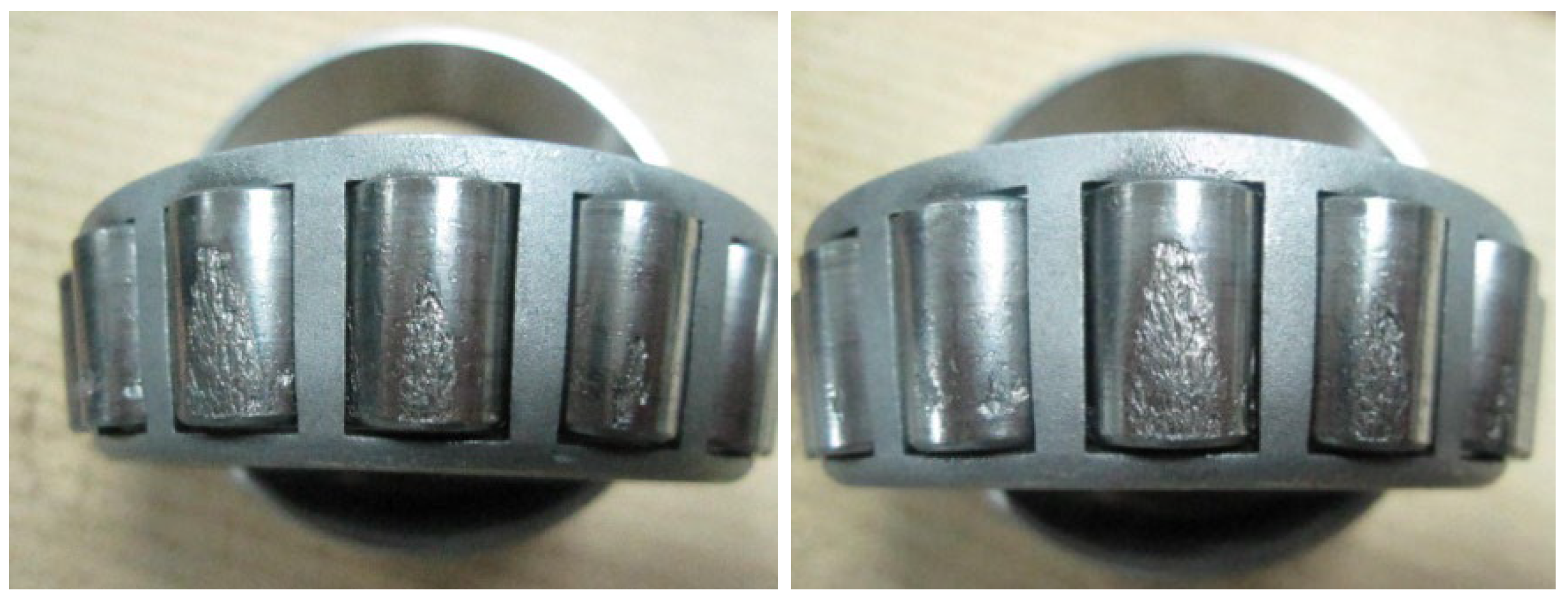
The vibration signal was exported and collected by the Lance LC0401 High Sensitivity ICP accelerometer and the YE6267 dynamic data collection and analysis system. The sampling frequency was 12 kHz per channel; 32,768 points is collected every five minutes. At the end of the test, the system fails with a rolling element defect, as illustrated in Figure 4.

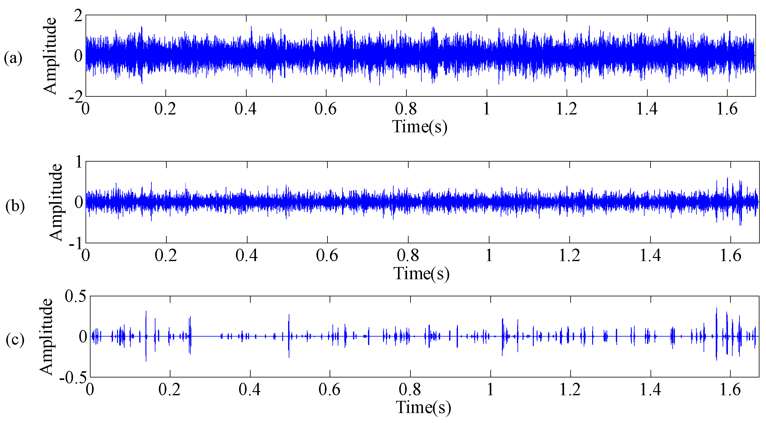
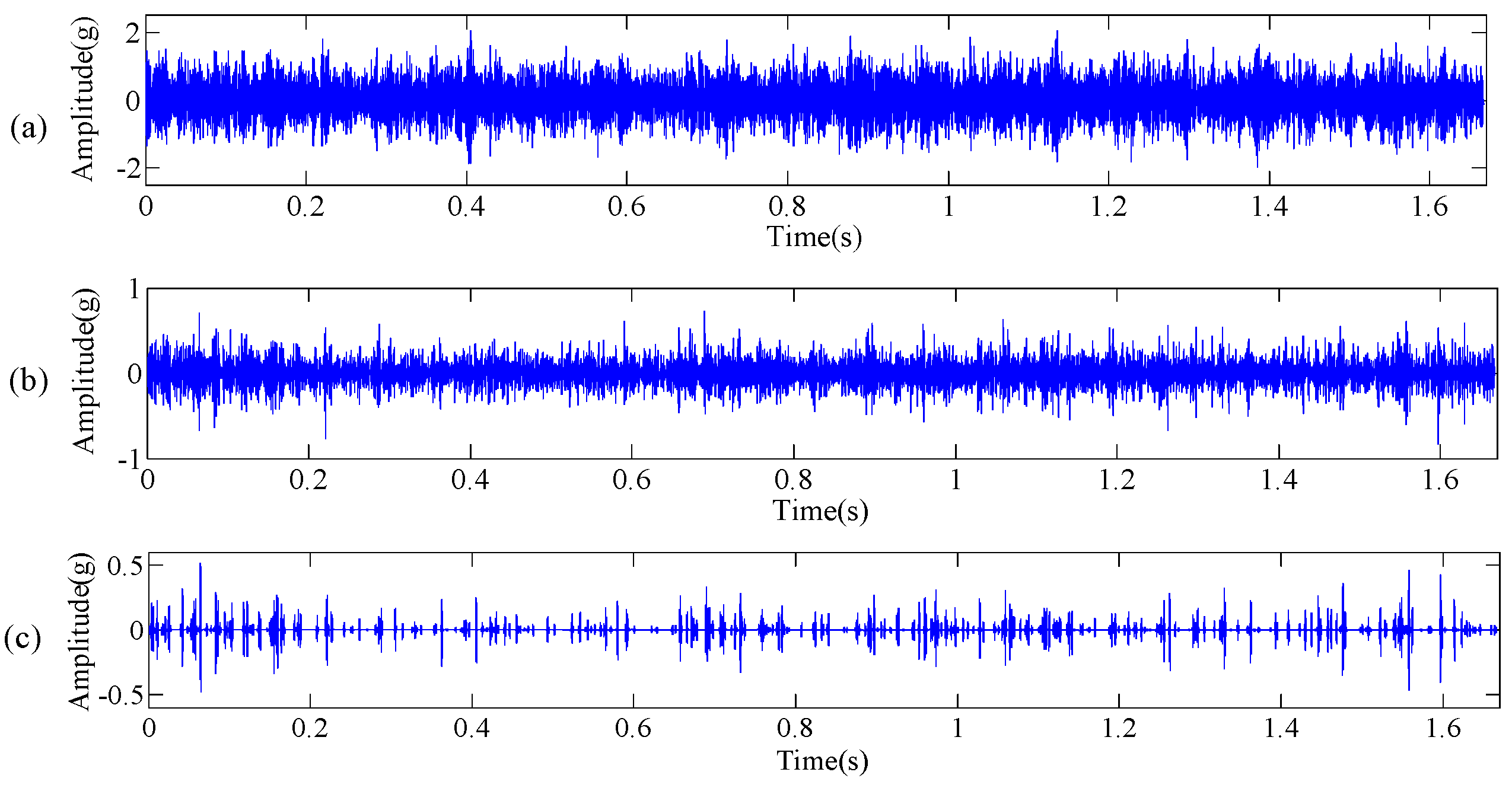
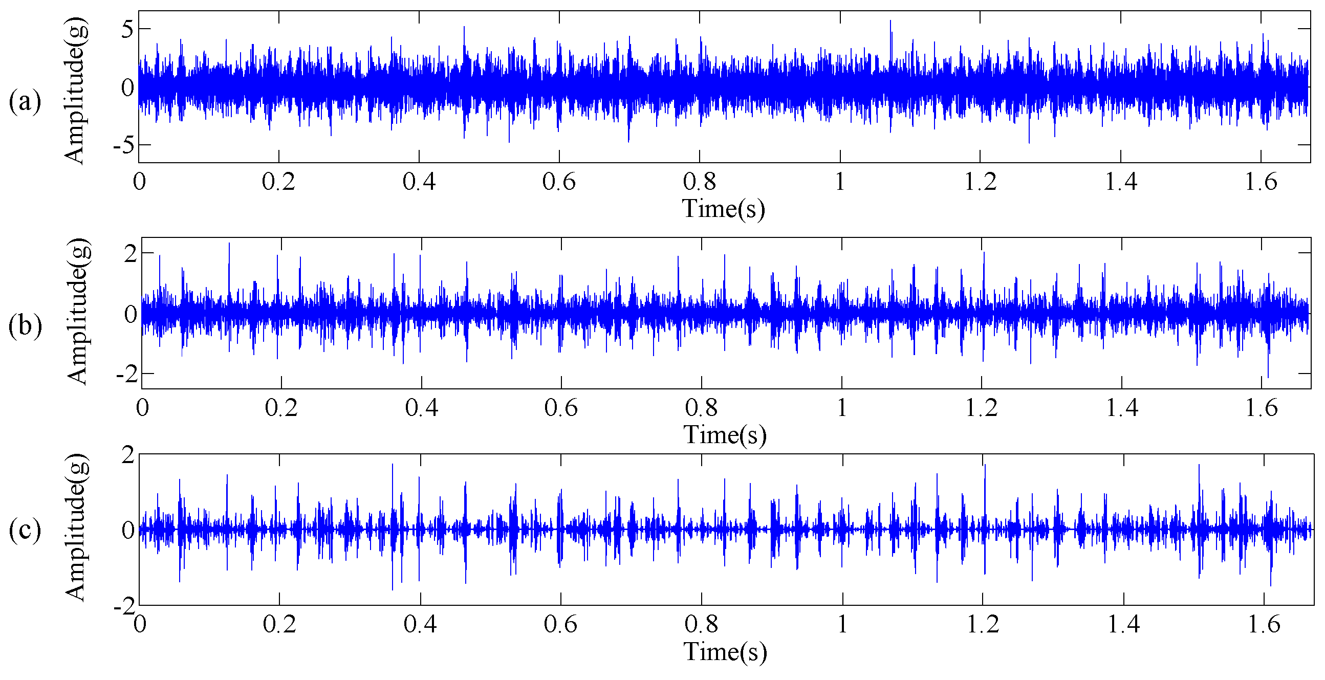
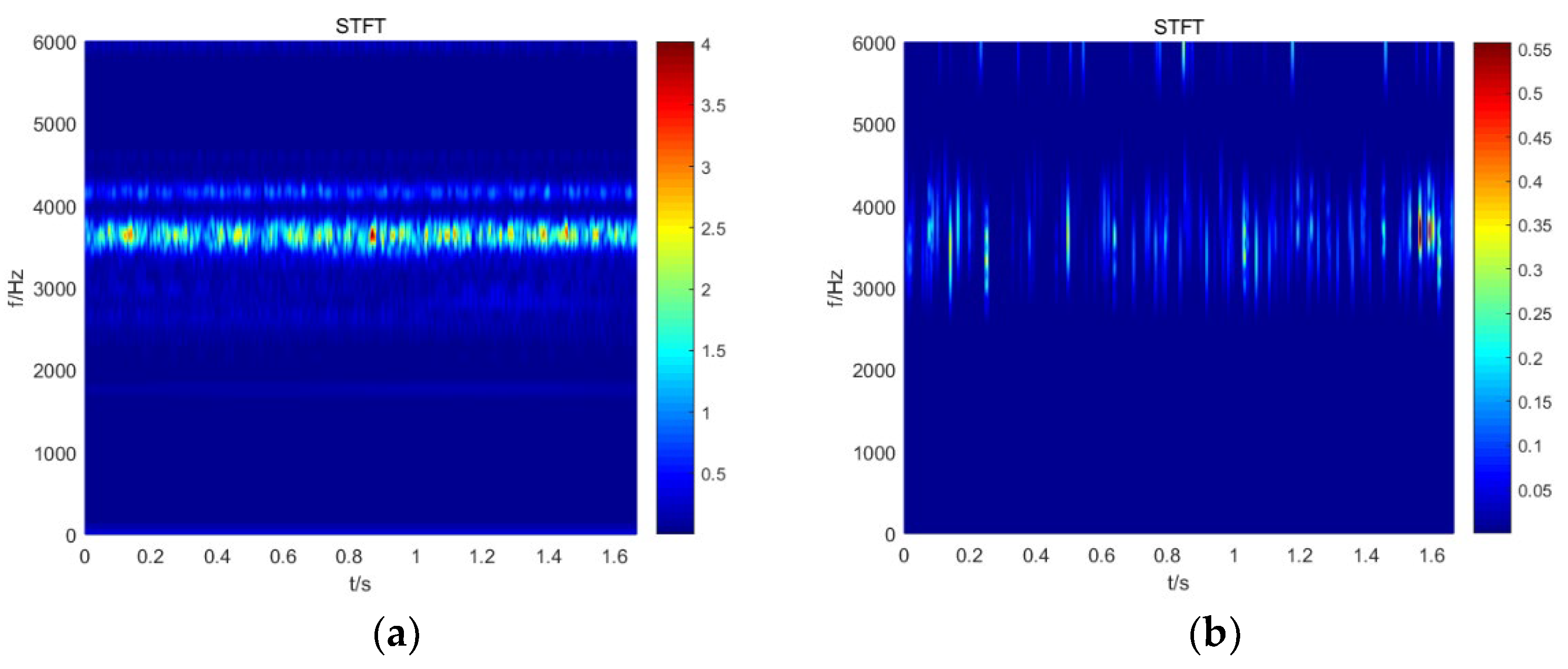
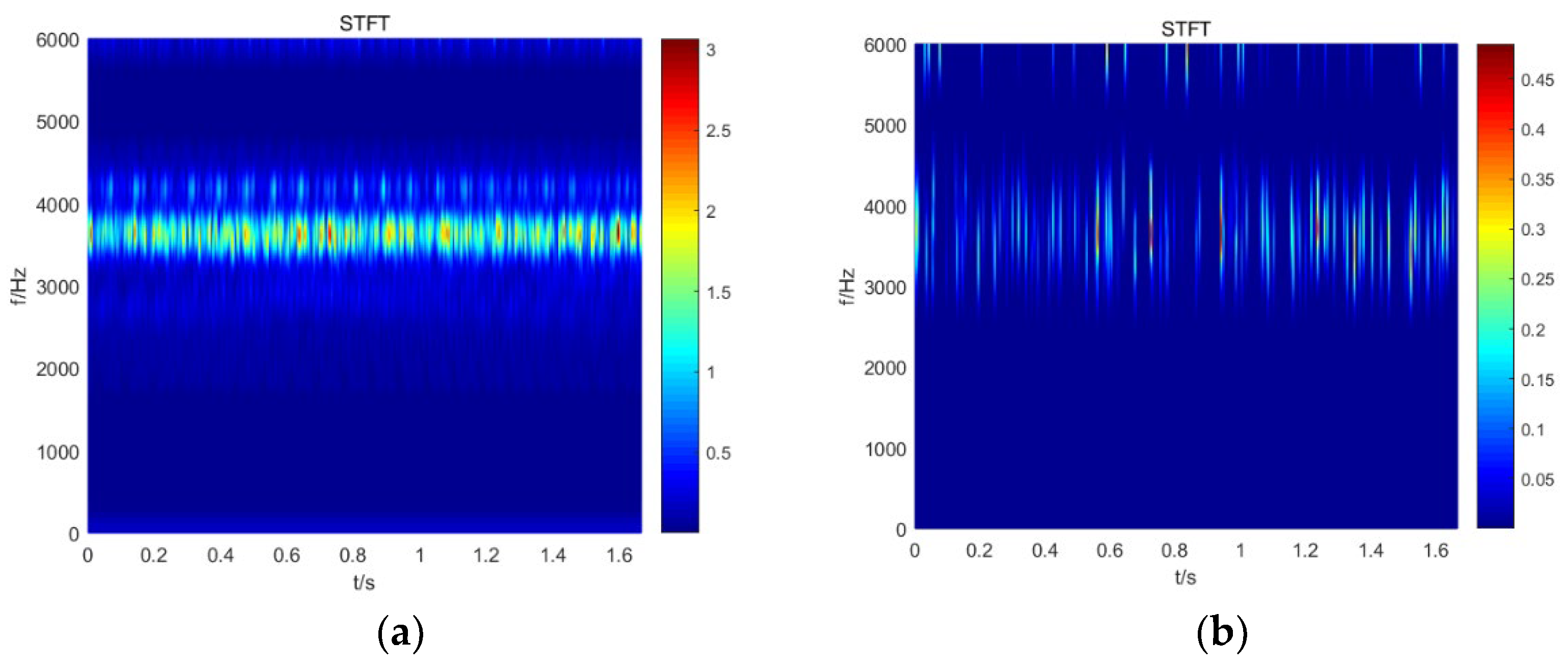
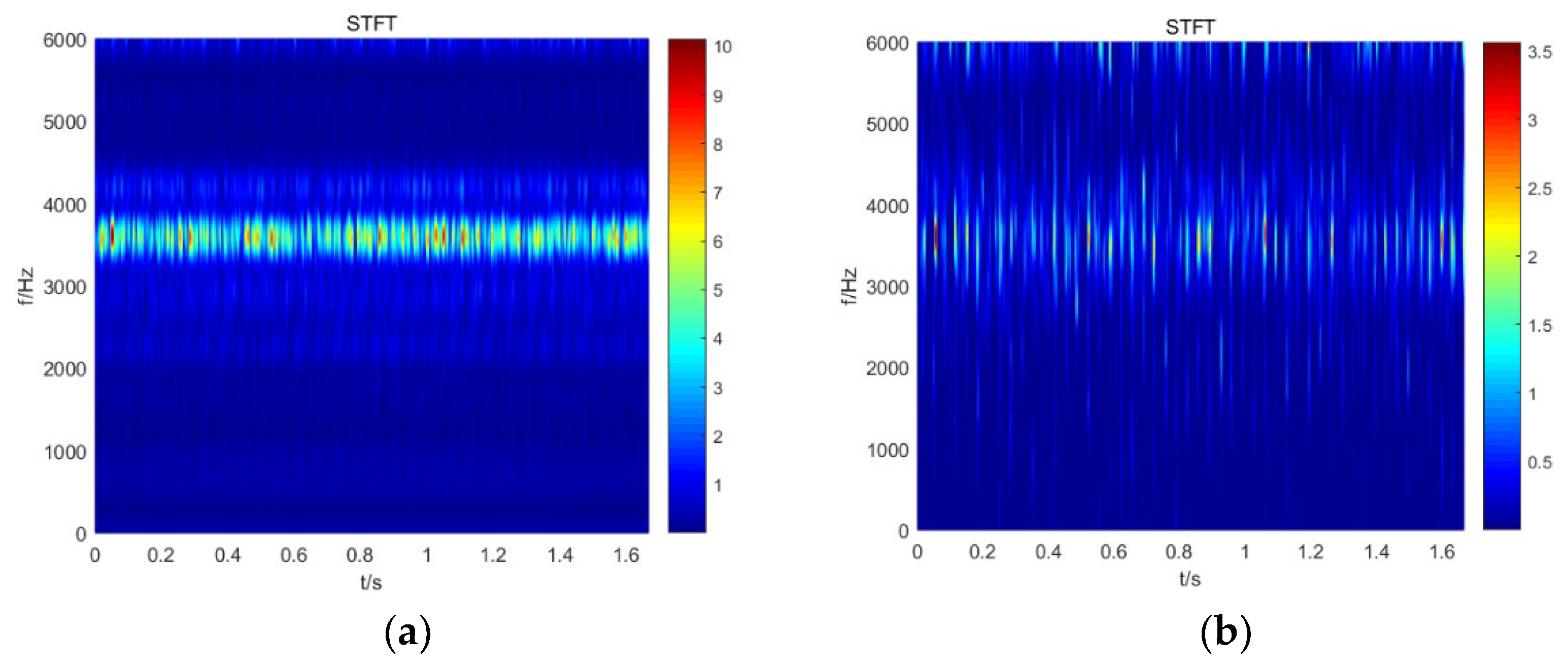
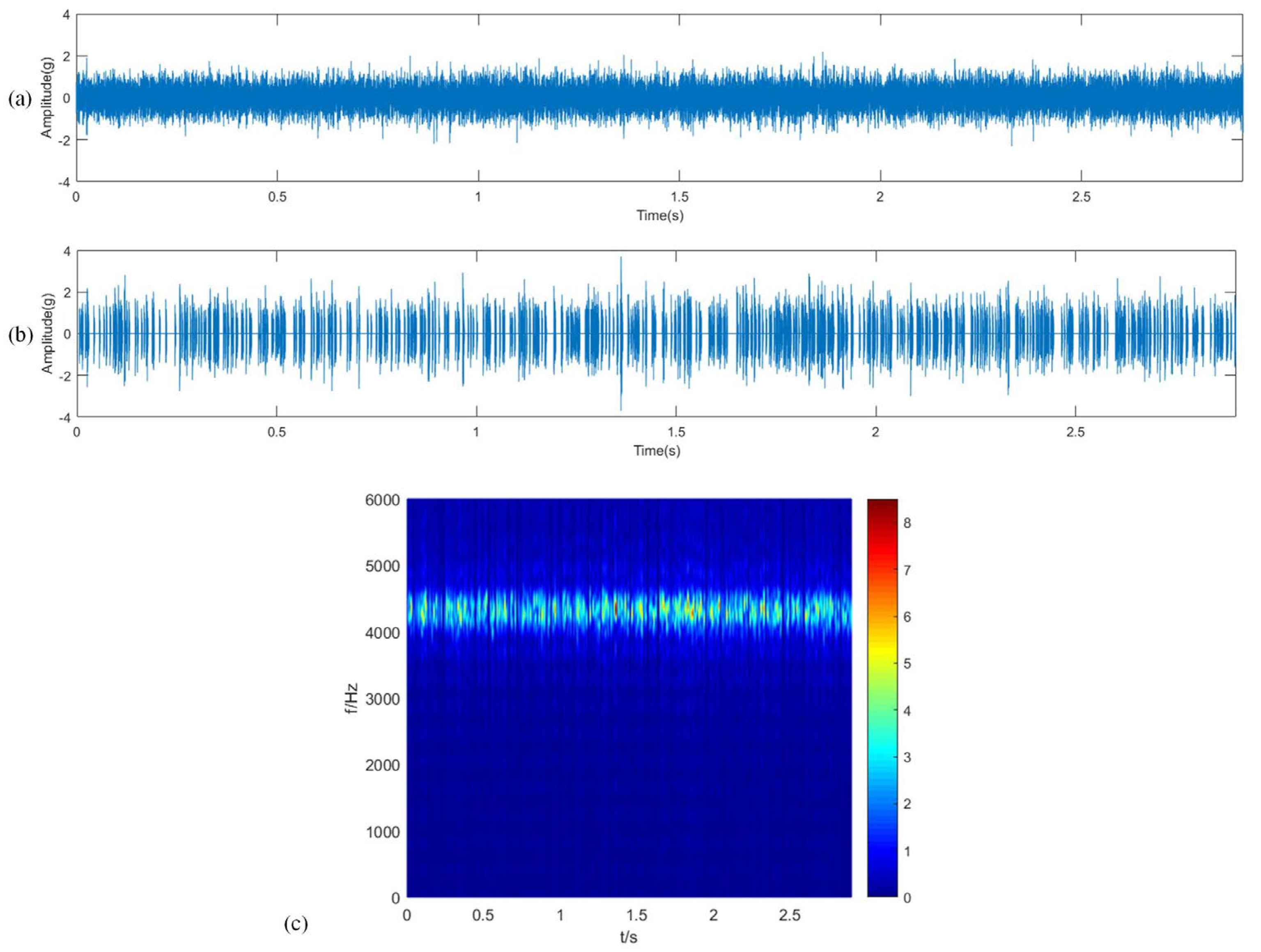
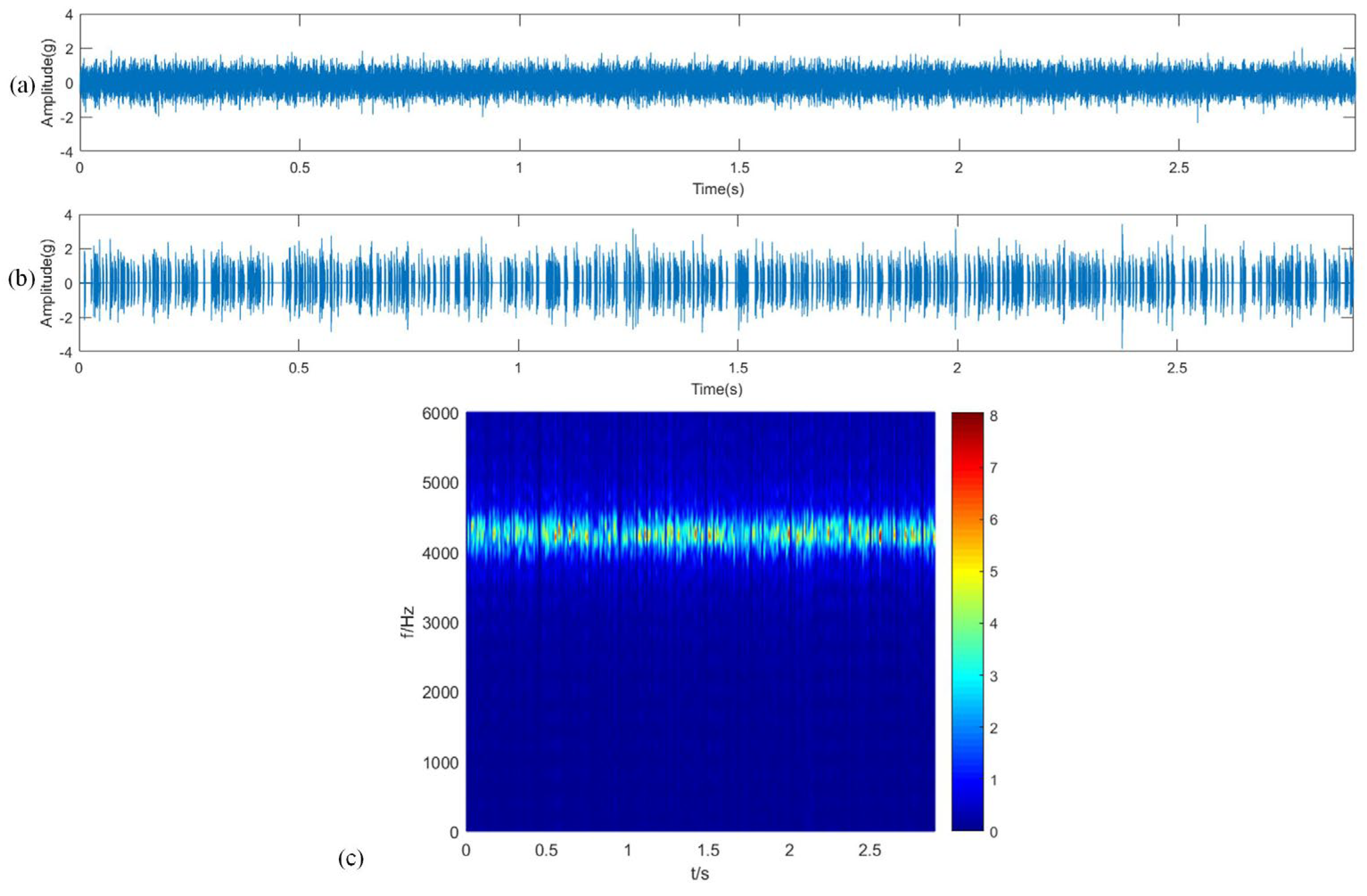
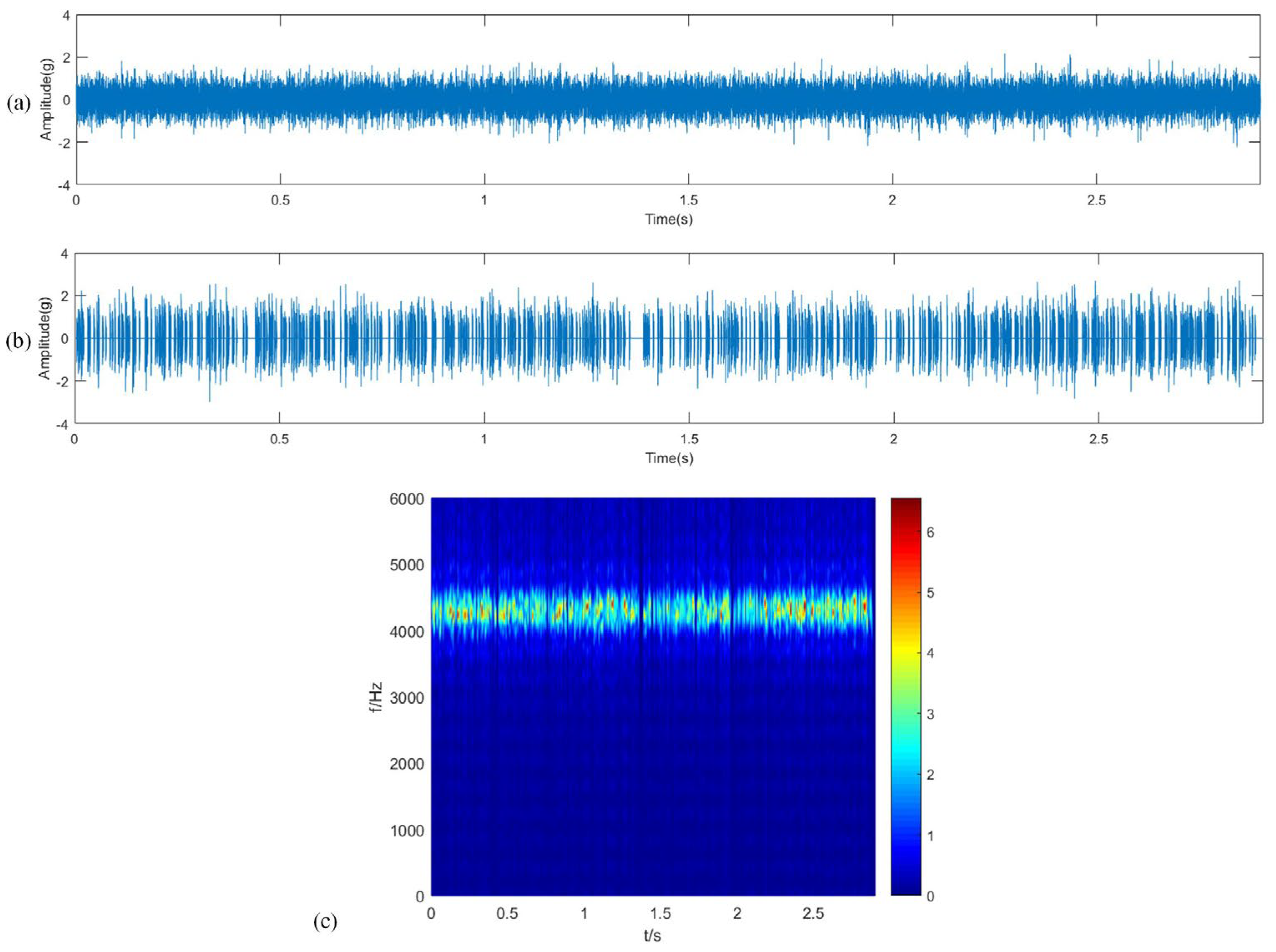
After the system failure, the vibration data were processed by Dual-BP and MCA, respectively. As with the previous case, three representative moments were analyzed: 25 h (300th group, normal stage), 60 h (533th group, incipient fault) and 95 h (1140th group, fault stage). The raw vibration signals and the reconstructed signals via Dual-BP and MCA are shown in Figure 5, Figure 6 and Figure 7, respectively. The short-time Fourier transform (STFT) of harmonic component and impulse component are shown in Figure 8, Figure 9 and Figure 10, respectively.

To verify the advantage of the proposed method, the same signals were analyzed via the state-of-the-art method in [28], which was constructed based on EMD and match pursuit. The raw vibration signals, the reconstructed signals, and the STFT of impulse component are shown in Figure 11, Figure 12 and Figure 13, respectively.

From Figure 5, Figure 6, Figure 7, Figure 8, Figure 9 and Figure 10, it can be seen that, after adding a penalty term to noise, MCA becomes more applicable for operational information extraction of the bearing–rotor system. Although the results of Dual-BP also reflect the fault degree, they are unsuitable as an index to reflect system reliability due to the serious noise interference. By comparison, the results of MCA are cleaner and more effective. Compared with the normal stage (Figure 5), the number of impulse components increased when faults occurred (Figure 6), although amplitudes did not substantially change. With the development of the fault, not only did the Impulse components increase in number, but their amplitudes also became larger (Figure 7). However, in Figure 11, Figure 12 and Figure 13, it is hard to distinguish the operational condition from the reconstructed component and the STFT results of impulse components via the comparison method. Therefore, the proposed method can extract more accurate operational information compared to the state-of-the-art method.

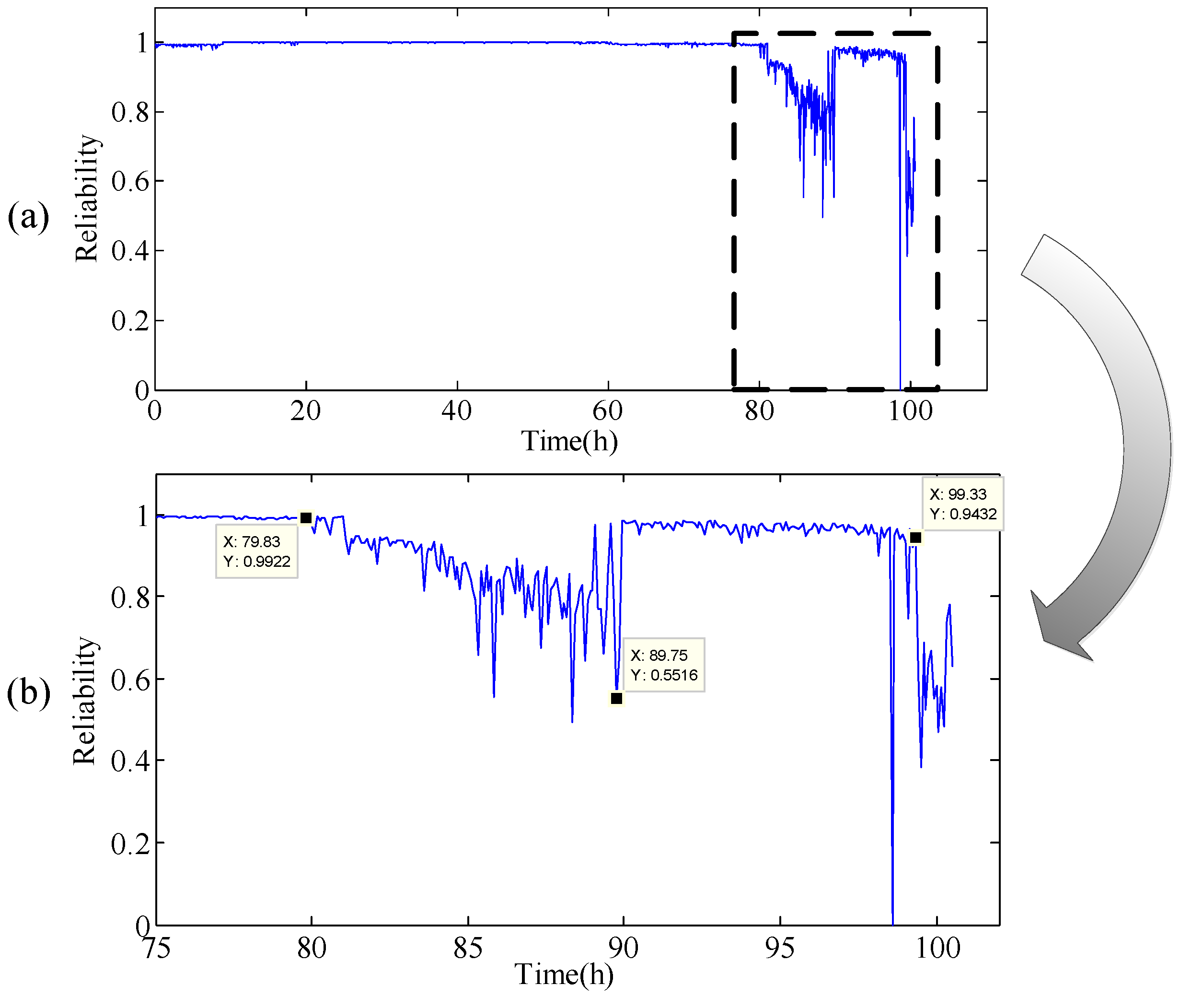
After sparse components separation, the few-shot reliability of the system can be calculated, as shown in Figure 14.

From Figure 14, it can be seen that the curve of reliability declines at 80 h. It can also be seen that the incipient fault occurred at this moment. While at 90 h, reliability rises to 0.98, which is the same case as example 1. This is because after running for a period, the defect was smoothed and the system ran smoothly again. Therefore, not only was the impulse component reduced, but also the vibration of all whole signals. After a slow decline, the value of reliability rapidly decreased to 0 at 96 h, which represented system failure. It can be seen that the proposed method can properly and accurately reflect the system condition.

In this study, we started from the system failure mechanism and discovered the vibration response of defects. Aiming to extract the fault vibration response, an MCA method was used for sparse components separation.

4. Conclusions

Traditional reliability estimation methods are mainly based on statistical analysis and life tests and may not be suitable for an increasingly diverse and precise set with high reliability requirements, which will be the inevitable result of the rapid development of technology and science. In this study, we started from the system failure mechanism and discovered the vibration response of defects. Aiming to extract the fault vibration response, an MCA method was used to extract the valuable component and remove other useless components or noise. Then, few-shot reliability could be estimated by the evaluation system and the output log-likelihood probability P(O|λ) of operational information sequence. Furthermore, this method does not rely on statistical analysis and large-failure samples because the evaluation process is accomplished by comparing the current condition with the normal condition of the same system. However, the construction of the basis relies on the vibration response of the bearing in this paper, which is still a scientific research gap that needs to be addressed.

References

- Wang, F.; Chen, X.; Liu, C.; Yan, D.; Li, H. Reliability assessment of rolling bearing based on principal component analysis and Weibull proportional hazard model. In Proceedings of the 2017 IEEE International Instrumentation and Measurement Technology Conference (I2MTC), Turin, Italy, 22–25 May 2017. [Google Scholar]
- Abaei, M.M.; Hekkenberg, R.; Bahootoroody, A. A multinomial process tree for reliability assessment of machinery in autonomous ships. Reliab. Eng. Syst. Saf. 2021, 210, 107484. [Google Scholar] [CrossRef]
- Varshney, L.; Vardhan, A.; Vardhan, A.; Kumar, S.; Sanjeevikumar, P. Performance characteristics and reliability assessment of self-excited induction generator for wind power generation. IET Renew. Power Gener. 2020, 15, 1927–1942. [Google Scholar] [CrossRef]
- Norouzi, N. The Pahlev Reliability Index: A measurement for the resilience of power generation technologies versus climate change. Nucl. Eng. Technol. 2021, 53, 1658–1663. [Google Scholar] [CrossRef]
- Cai, G.; Chen, X.; Li, B.; Chen, B. Operation reliability assessment for cutting tools by applying a proportional covariate model to condition monitoring information. Sensors 2012, 12, 12964–12987. [Google Scholar] [CrossRef] [Green Version]
- Hu, B.; Pan, C.; Shao, C.; Xie, K.; Niu, T.; Li, C.; Peng, L. Decision-Dependent Uncertainty Modeling in Power System Operational Reliability Evaluations. IEEE Trans. Power Syst. 2021, 36, 5708–5721. [Google Scholar] [CrossRef]
- Qc, A.; Cz, A.; Zhao, Y.; Yan, X.B. Operational reliability assessment of photovoltaic inverters considering voltage/VAR control function. Electr. Power Syst. Res. 2021, 190, 106706. [Google Scholar]
- Ren, Z.; Zhu, Y.; Yan, K.; Chen, K.; Kang, W.; Yue, Y.; Gao, D. A novel model with the ability of few-shot learning and quick updating for intelligent fault diagnosis. Mech. Syst. Signal Process. 2020, 138, 106608.1–106608.21. [Google Scholar] [CrossRef]
- Hu, Y.; Liu, R.; Li, X.; Chen, D.; Hu, Q. Task-Sequencing Meta Learning for Intelligent Few-Shot Fault Diagnosis With Limited Data. IEEE Trans. Ind. Inform. 2022, 18, 3894–3904. [Google Scholar] [CrossRef]
- Chen, H.; Liu, R.; Xie, Z.; Hu, Q.; Dai, J.; Zhai, J. Majorities help minorities: Hierarchical structure guided transfer learning for few-shot fault recognition. Pattern Recognit. 2022, 123, 108383. [Google Scholar] [CrossRef]
- Liu, R.; Yang, B.; Zhang, X.; Wang, S.; Chen, X. Time-frequency atoms-driven support vector machine method for bearings incipient fault diagnosis. Mech. Syst. Signal. Process. 2016, 75, 345–370. [Google Scholar] [CrossRef]
- Niu, L.; Cao, H.; He, Z.; Li, Y. Dynamic modeling and vibration response simulation for high speed rolling ball bearings with localized surface defects in raceways. J. Manuf. Sci. Eng. 2014, 136, 041015. [Google Scholar] [CrossRef]
- Li, Y.; Cao, H.; Chen, X. Modelling and vibration analysis of machine tool spindle system with bearing defects. Int. J. Mechatron. Manuf. Syst. 2015, 8, 33–48. [Google Scholar] [CrossRef]
- Chen, S.S.; Donoho, D.L.; Saunders, M.A. Atomic decomposition by basis pursuit. SIAM J. Sci. Comput. 1998, 20, 33–61. [Google Scholar] [CrossRef]
- Elad, M.; Milanfar, P.; Rubinstein, R. Analysis versus synthesis in signal priors. Inverse Probl. 2007, 23, 947. [Google Scholar] [CrossRef] [Green Version]
- Starck, J.L.; Elad, M.; Donoho, D. Redundant multiscale transforms and their application for morphological component separation. Adv. Imaging Electron. Phys. 2004, 132, 287–348. [Google Scholar]
- Starck, J.L.; Elad, M.; Donoho, D.L. Image decomposition via the combination of sparse representations and a variational approach. IEEE Trans. Image Process. 2005, 14, 1570–1582. [Google Scholar] [CrossRef] [PubMed] [Green Version]
- Daubechies, I.; Defrise, M.; Mol, C.D. An iterative thresholding algorithm for linear inverse problems with a sparsity constraint. Commun. Pure Appl. Math. 2010, 57, 1413–1457. [Google Scholar] [CrossRef] [Green Version]
- Sardy, S.; Tseng, B.P. Block coordinate relaxation methods for nonparametric wavelet denoising. J. Comput. Graph. Stat. 2000, 9, 361–379. [Google Scholar]
- Baruah, P.; Chinnam, R.B. HMMs for diagnostics and prognostics in machining processes. Int. J. Prod. Res. 2005, 43, 1275–1293. [Google Scholar] [CrossRef]
- Chinnam, R.B.; Baruah, P. Autonomous diagnostics and prognostics through competitive learning driven HMM-based clustering. In Proceedings of the International Joint Conference on Neural Networks, Portland, OR, USA, 20–24 July 2003; Volume 4, pp. 2466–2471. [Google Scholar]
- Wang, Y.; Yan, H.; Zhang, H.; Shen, H.; Lam, H.K. Interval Type-2 Fuzzy Control for HMM-Based Multiagent Systems Via Dynamic Event-Triggered Scheme. IEEE Trans. Fuzzy Syst. 2021. [Google Scholar] [CrossRef]
- Tobon-Mejia, D.A.; Medjaher, K.; Zerhouni, N.; Tripot, G. A data-driven failure prognostics method based on mixture of gaussians hidden markov models. IEEE Trans. Reliab. 2012, 61, 491–503. [Google Scholar] [CrossRef] [Green Version]
- Deng, Q.; Söffker, D. A Review of the current HMM-based Approaches of Driving Behaviors Recognition and Prediction. IEEE Trans. Intell. Veh. 2021. [Google Scholar] [CrossRef]
- Li, F.; Zheng, W.X.; Xu, S. HMM-Based fuzzy control for nonlinear Markov jump singularly perturbed systems with general transition and mode detection information. IEEE Trans. Cybern. 2021. [Google Scholar] [CrossRef]
- Lee, W.L.J.; Burattin, A.; Munoz-Gama, J.; Sepúlveda, M. Orientation and conformance: A HMM-based approach to online conformance checking. Inf. Syst. 2021, 102, 101674. [Google Scholar] [CrossRef]
- Sun, C.; Zhang, Z.; He, Z.; Shen, Z.; Chen, B.; Xiao, W. Novel method for bearing performance degradation assessment—A kernel locality preserving projection based approach. Proc. Inst. Mech. Eng. Part C J. Mech. Eng. Sci. 2014, 228, 548–560. [Google Scholar] [CrossRef]
- Liu, Z.; Ding, K.; Lin, H.; He, G.; Du, C.; Chen, Z. A Novel Impact Feature Extraction Method Based on EMD and Sparse Decomposition for Gear Local Fault Diagnosis. Machines 2022, 10, 242. [Google Scholar] [CrossRef]
Figure 1.
Flowchart of the few-shot reliability assessment approach.
Figure 2.
The acceleration response when the defect is on the outer raceway.
Figure 3.
The acceleration response when the defect is on the inner raceway.
Figure 4.
Defects of the failure bearings.
Figure 5.
In 25 h: (a) Raw vibration signals; (b) reconstructed component via Dual−BP; (c) reconstructed component via MCA.
Figure 6.
In 60 h: (a) Raw vibration signals; (b) reconstructed component via Dual−BP; (c) reconstructed component via MCA.
Figure 7.
In 95 h: (a) Raw vibration signals; (b) reconstructed component via Dual−BP; (c) reconstructed component via MCA.
Figure 8.
In 25 h: the STFT of (a) harmonic component; (b) impulse component.
Figure 9.
In 60 h: the STFT of (a) harmonic component; (b) impulse component.
Figure 10.
In 95 h: the STFT of (a) harmonic component; (b) impulse component.
Figure 11.
In 25 h: (a) Raw vibration signals; (b) reconstructed component; (c) the STFT of impulse component.
Figure 12.
In 60 h: (a) Raw vibration signals; (b) reconstructed component; (c) the STFT of impulse component.
Figure 13.
In 95 h: (a) Raw vibration signals; (b) reconstructed component; (c) the STFT of impulse component.
Figure 14.
(a) Few-shot reliability estimation result via statistical indexes; (b) local enlargement.
Publisher’s Note: MDPI stays neutral with regard to jurisdictional claims in published maps and institutional affiliations. |
© 2022 by the authors. Licensee MDPI, Basel, Switzerland. This article is an open access article distributed under the terms and conditions of the Creative Commons Attribution (CC BY) license (https://creativecommons.org/licenses/by/4.0/).
Share and Cite
MDPI and ACS Style
Feng, Y.; Li, W.; Zhang, K.; Li, X.; Cai, W.; Liu, R. Morphological Component Analysis-Based Hidden Markov Model for Few-Shot Reliability Assessment of Bearing. Machines 2022, 10, 435. https://doi.org/10.3390/machines10060435
AMA Style
Feng Y, Li W, Zhang K, Li X, Cai W, Liu R. Morphological Component Analysis-Based Hidden Markov Model for Few-Shot Reliability Assessment of Bearing. Machines. 2022; 10(6):435. https://doi.org/10.3390/machines10060435
Chicago/Turabian StyleFeng, Yi, Weijun Li, Kai Zhang, Xianling Li, Wenfang Cai, and Ruonan Liu. 2022. "Morphological Component Analysis-Based Hidden Markov Model for Few-Shot Reliability Assessment of Bearing" Machines 10, no. 6: 435. https://doi.org/10.3390/machines10060435
Note that from the first issue of 2016, this journal uses article numbers instead of page numbers. See further details here.