1. Introduction
The pipe assembly process is commonly encountered in various fields, such as the aircraft, aerospace, and ship building industries. Pipe assembly plays an important role in product quality, including the safety, reliability, performance, and life cycle of the product [
1]. In an aero-engine, approximately 50 accessories, hundreds of clamps, and 100–250 pipes exist within the narrow space between the engine casing and nacelle. These pipes connect the engine components, accessories, and aircraft to transmit fluids and ensure that the engine operates. Academic researchers and practitioners in engineering disciplines generally pay considerable attention to pipe routing algorithms in the field of pipe assembly design [
2]. Pipe routing is a time-consuming and difficult task, even for skilled designers, owing to the complexity of 3D space and the vast amount of engineering rules involved, such as avoiding obstacles, closely following obstacle contours, and meeting assembly feasibility requirements. In practice, there are equally significant difficulties in pipe assembly production. Certain digital assembly and measurement techniques have been realized. For example, a simulation technology for the pipe bending process has been applied to collision detection [
3]. A 3D measurement system for pipe assembly was developed to improve the assembly productivity and accuracy [
4]. Simulation of the pipe assembly process has been utilized for interference checking and sequence optimization in pipe assembly [
5].
Aimed at locating and clamping different pipe types during assembly, a flexible combine-clamp and flexible pipe assembly platform represent a good solution. Moreover, pipe recognition and measurement systems [
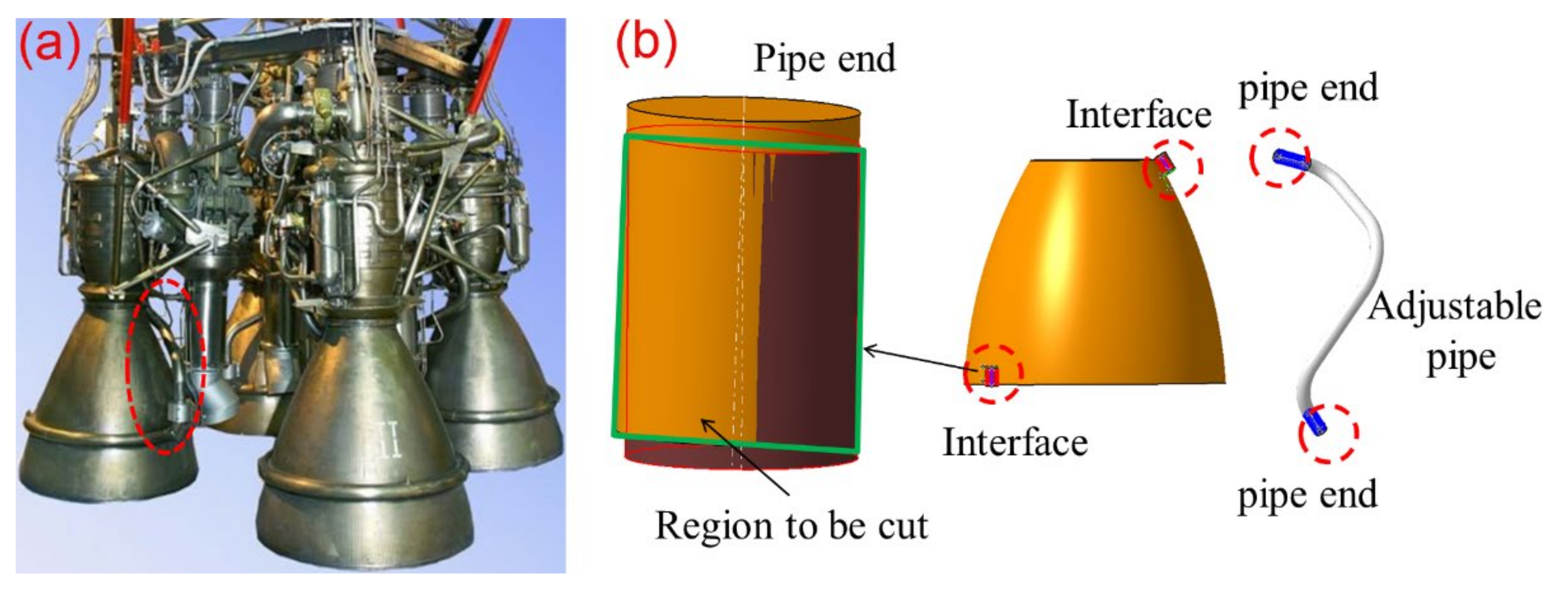
6] were used to calculate and control robot motion in an automatic pipe assembly system. However, the production of pipe assembly for a rocket engine not only experiences similar difficulties, but is also even more challenging, owing to the higher requirements of the joining and sealing performance. In the production of a rocket engine, welding is the preferred process for connecting pipes, components, and accessories. In comparison with a threaded connection, welding offers superior sealing performance, which directly affects the rocket engine safety and reliability. Meanwhile, errors after welding are inevitable and easily propagated during production, which often result in the pipe ends not fitting into their corresponding interfaces located at the “closing” segment (see
Figure 1). In order to compensate for these production errors, which often result in rework and slow assembly, appropriate steps could be considered. First, the design for assembly (DFA) approaches, employing tolerance analyses, could be utilized to minimize errors [
7]. DFA is an important engineering technique in machining and assembly process planning, and such methods offer an effective procedure for error evaluation. Nevertheless, it is difficult to predict welding distortions, which makes this approach ineffective in reducing production errors. Similarly, flexible assembly and welding platforms could be developed to improve the location and clamping of different pipe types. However, errors after welding still exist and cannot yet be completely reduced. Therefore, using a pipe adjustment tool (“forced closing”) is a common approach for solving the accumulating errors located at the “closing” segment. However, this method is only suitable for minor production errors and requires further investigation on the installation stress and strain to avoid exceeding the allowable values [
8]. Large installation stresses caused by major production errors, coupled with welding residual stress and dynamic loading located at the “closing” segment, will directly reduce rocket engine safety and reliability. An adjustable pipe is a flexible and economical means of compensating for major production errors (see
Figure 1). For welding purposes, the pipe ends are normally longer. Therefore, a certain portion of each end should be cut off to match the corresponding interface, as shown in
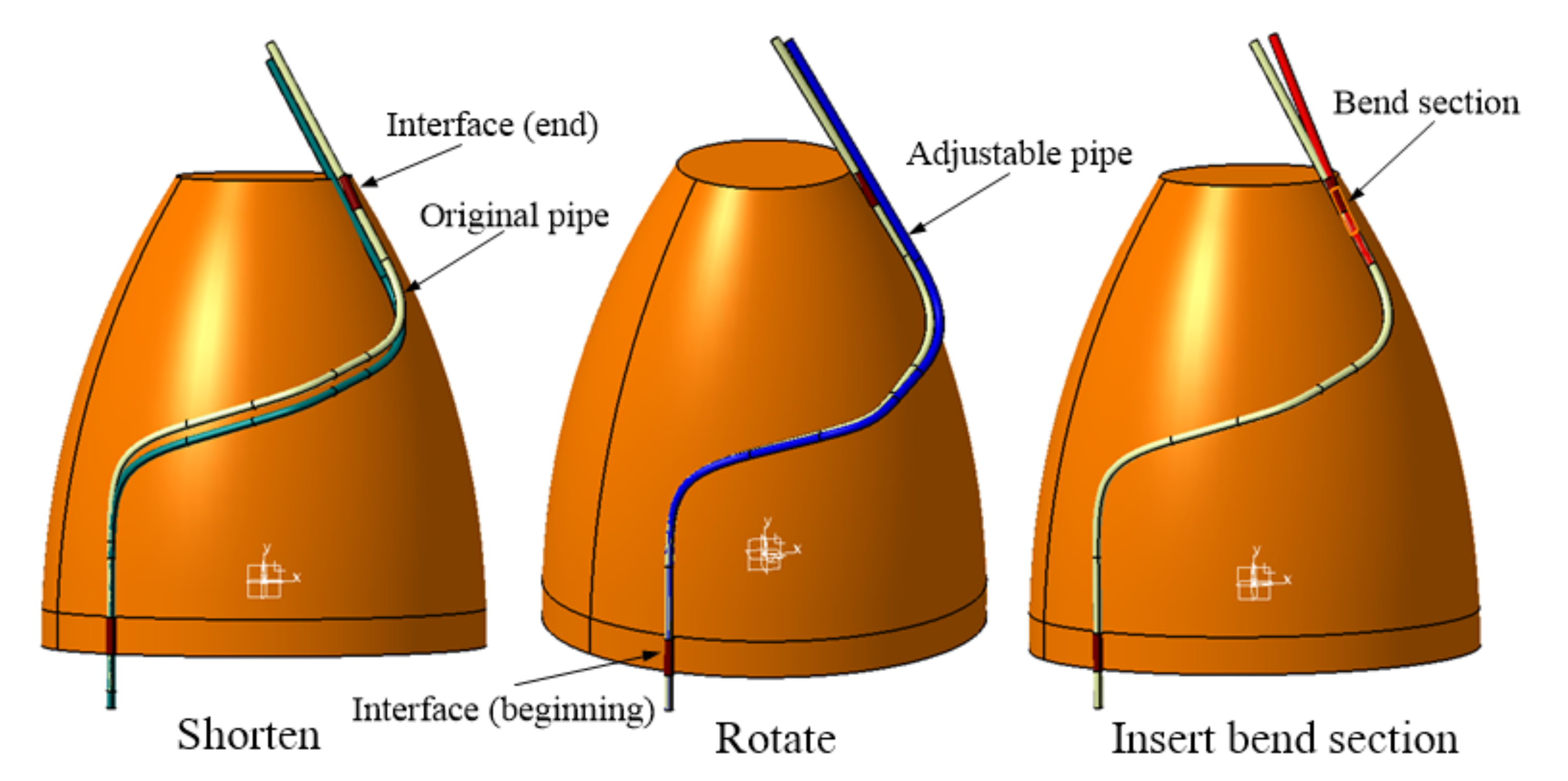
Figure 1. Moreover, when faced with major production errors, a useful approach of inserting a bend section could be executed, as illustrated in
Figure 2.
Formally, using an adjustable pipe to compensate for production errors involves the following three sub-problems:
- (i)
Collecting real-time 3D information, including the limited installation space, the 3D shape of the adjustable pipe, and 3D pose of interfaces;
- (ii)
Meeting the requirements of the welding axis alignment for each pipe end; and
- (iii)
Calculating the final pose of the adjustable pipe, cutting length of each end, and bending parameters.
As can be seen in
Figure 2, if the axis is aligned at one of the ends, three different approaches can be executed to adjust the pose of the other end to match the corresponding interface. The first option is to shorten the beginning of the pipe, which represents one translational degree of freedom (DOF), as shown in
Figure 2. The second alternative is to rotate around the axis of the beginning segment and represent one rotational DOF. The third possibility is to insert a bend section located at the beginning or end of the pipe, which indicates three DOFs (namely, position, orientation, and angle). However, considering nonlinear coupling in 3D space when using multiple adjustment approaches, and the welding axis alignment requirement of the pipe end, it is often difficult to finish the process manually.
To improve the productivity and accuracy of the adjustable pipe in this work, inline measurements systems are integrated into production to develop an adaptive control system. Cost-efficient inline 3D sensing technologies, such as laser scanning and digital photogrammetry, are currently available to gather real-time 3D information [
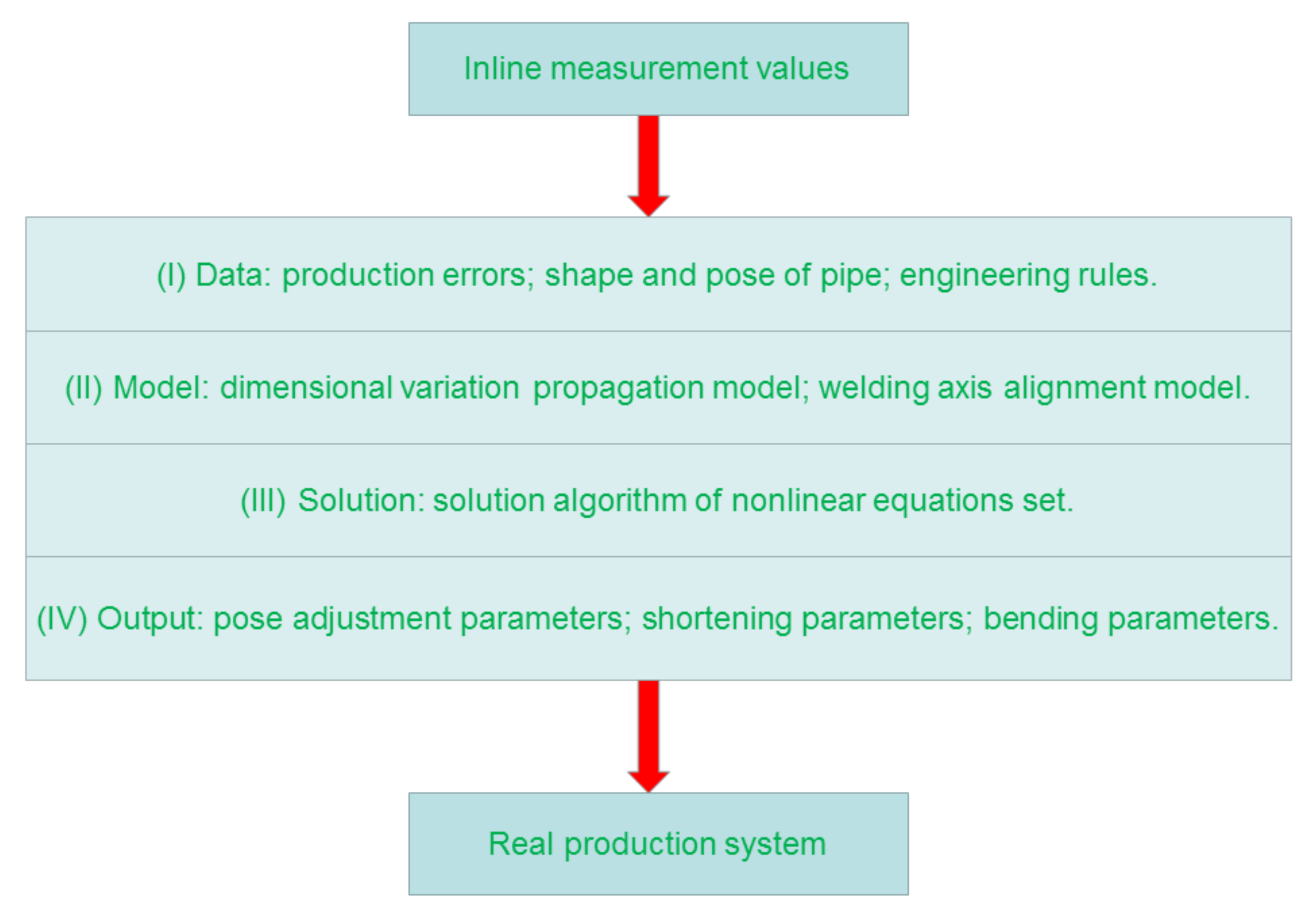
9]. In this study, dimensional chains analyses are used to evaluate the nonlinear coupling in 3D space when using multiple approaches. A dimensional variation propagation model is established to describe the geometric relationship between the adjustment approaches and pipe end. The welding axis alignment requirement is modeled to describe the motion/displacement (that is, the position and orientation) between the pipe end and corresponding interface. In general, the proposed adaptive control system described in this research, as illustrated in
Figure 3, consists of the following four levels:
Data: The production errors as well as the shape and pose of the adjustable pipe should be extracted from the inline measurement data. Furthermore, various engineering rules exist, such as the maximum shortening length of each pipe end.
Model: Using the real-time data from the previous step, a dimensional variation propagation model needs to be developed. The welding axis alignment requirement of the pipe end also needs to be described and modeled.
Solution: The nonlinear equation set between the established models must be solved under geometric constraints and engineering rules.
Output: Local feedback parameters required for the necessary adjustment approaches must be arranged using the global calculation results obtained from the previous step. These include shortening lengths, rotate angle, and bending parameters.
The remainder of this paper is organized as follows. The models and solution method of adjustable laser bending pipe [
10,
11,
12] to compensate for pipe assembly production errors are provided in
Section 2. Experimental results and discussions are presented in
Section 3 to verify the feasibility and accuracy of the proposed adaptive control system, and the paper is concluded in
Section 4.
2. Models and Solution
The matching method [
13,
14] was used in the adaptive control algorithm of lightweight space-frame-structures, which are increasingly being used in the automobile and aircraft industries. Meanwhile, in building construction, a kinematics model of a pipeline with multiple pipes was established for automatic realignment by means of the Denavit–Hartenberg (D-H) matrix [
15]. However, when faced with major production errors, the specific position and orientation of an inserted bend section are uncertain, making it difficult to establish the local D-H parameters and to extract the key point from the measurement data of the adjustable pipe required in the matching method. In this study, the production of exponentials (POE) formula is an alternative method and is used to model dimensional chains when using multiple adjustment approaches. In a global POE formula, all kinematics chains are related to the inertial frame and only two coordinate frames are required: a spatial frame {S} and tool frame {T} [
16].
In this section, robotic kinematics studies are first introduced, and then the dimensional variation propagation model is developed along with the required functions, and the welding axis alignment model is also described combined with the incompletely specified displacement screw system related theories. Finally, the solution method is presented to solve the nonlinear equation set between the established models.
2.1. Robotic Kinematics
Robotic kinematics describes the position and orientation of the end-effector connected by robotic joints, and includes two robotic kinematics problems [
17]. Forward robotic kinematics generally refers to describing the relationship between the variables (joint angles and displacements) and end effector pose (position and orientation) in robotic systems. Meanwhile, inverse kinematics generally refers to the calculation of variables for a given end effector pose. That is, forward robotic kinematics aims to model the nonlinear coupling relationship between joints and end effector pose, while inverse kinematics provides the corresponding solution method. Generally, the forward robotic kinematics can be expressed based on the POE formula [
18], as follows:
where
,
are joint variables;
is the initial pose; and
,
represent the joint screw in the form of
In the above,
is the usual cross-product of 3D vector algebra;
is a unit vector defined on the joint axis;
is a vector directing the point O to an arbitrary point on the joint axis; and
h is the screw pitch [
18], as shown in
Figure 4.
For pure rotation, the screw can be expressed as
For pure translation, the screw can be expressed as
Moreover, it is common to use Newton–Raphson iterative methods for inverse kinematics [
19], based on computation of the Jacobian matrix. When using the POE formula, the Jacobian matrix has the following linear form:
2.2. Dimensional Variation Propagation Model of Adjustable Pipe
The dimensional variation propagation model of the adjustable pipe describes the geometric relationship between the adjustment approaches and pipe end in the global frame. As illustrated in
Figure 5, when using multiple adjustment approaches shown in
Figure 2, the kinematics chains model can be expressed by three joint screws:
,
, and
, respectively.
is a translation screw, which results from the one-translation DOF by means of shortening the beginning of the pipe, and can be described using the global POE formula:
where
represents the shortening length of the beginning of the pipe; both d
1 and d
2 are constant numbers and depend on the actual installation space; and
is the unit orientation vector of the beginning segment axis of the pipe.
is a rotation screw, which results from the one-rotation DOF by rotating around the beginning segment axis, and can be written as follows:
where
is a rotation screw;
represents the rotation angle around the axis of the beginning of the pipe; both
and
are constant numbers and depend on the actual installation space; P is an arbitrary point located on the axis of the beginning of the pipe (see
Figure 5); and
is the unit orientation vector of the axis of the beginning of the pipe.
is a screw that results from the third approach of inserting a bend section located at the end or beginning of the pipe. Owing to the elastic recovery of the pipe, significant spring-back occurs following the plastic pipe bending process, which leads to an increase in the bending radius and a decrease in the bending angle [
20]. This has a significant influence on the bend section shape. Laser bending is a new flexible forming process that is free of spring-back [
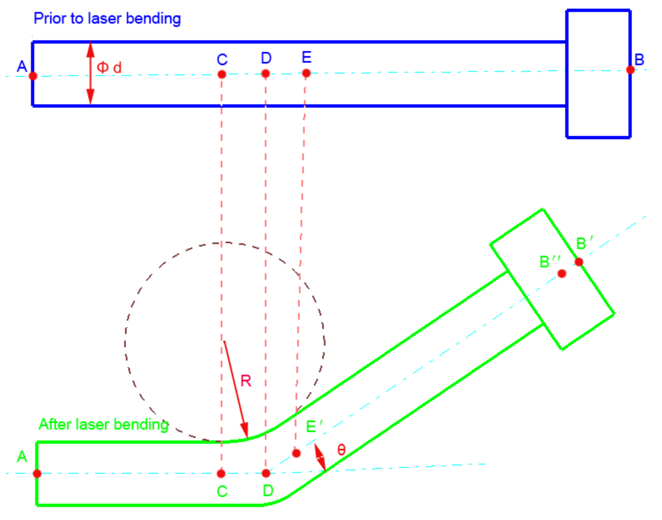
21]. In this study, pipe laser bending is used to verify the geometric accuracy of the established model. A schematic of the equivalent motion of a 2D bend section is presented in
Figure 6a, in which a pipe segment AB with pipe diameter d is irradiated by a laser beam on CE, and a bend section with bending angle and bending radius R + d/2 is obtained. In addition, pipe end B moves to
. A bend section sample using pipe laser bending is shown in
Figure 6b.
The equivalent motion of the pipe end when inserting a bend section can be described by using the syntheses of two basic motions: the rotation of end B around point D to point with angle , and the translation of along the axial direction of the pipe to .
Assuming that the neutral layers of a bend section are invariable,
Combining Equation (10) through (13) yields
As can be seen from
Figure 7, when considering a bend section located in a 3D space, three bending parameters exist, including the bending position
, bending orientation
, and bending angle
, which is the equivalent bend-rotation point. A 3D straight pipe
can be represented as
, where
is the unit orientation vector of the segment
;
is the foot of the perpendicular through origin point o of
;
is the distance between points
and
along
; and
represents the bending angle. Combined with Equation (14),
can be expressed as follows.
In the above,
is the unit orientation vector of the perpendicular of
;
is the cross-product of
and
;
represents the included angle between
and
around the axis of the pipe
; and the bending orientation
can be expressed as
is the syntheses screw of bending, and can be divided into
and
, where
is a screw of equivalent bending-rotation and
is a screw of equivalent bending-translation, and can be expressed as follows:
In summary, the dimensional chains of the third approach of inserting a bend section can be described using Equation (14) in the form of Equation (1)
With the established kinematics models of the three approaches, respectively, including Equations (6), (8), and (20), the dimensional variation propagation model when using three different adjustment approaches includes five adjustable DOFs, and can be written as in the form of Equation (1)
where
represents the shortening length of the beginning of the pipe;
is the rotation angle around the axis of the beginning of the pipe;
represents the bending angle;
is the included angle between the orientation vectors
and
around the axis of the pipe;
is the distance between points
and
along the axial direction of the pipe; both d
1 and d
2 are constant numbers that depend on the actual pipeline assembly space;
and
are constant numbers that depend on the actual installation space; and
and
are constant numbers that depend on the actual pipe shape.
2.3. Welding Axis Alignment Model of Pipe End
The welding axis alignment model of the pipe end describes the motion/displacement (i.e., position and orientation) between the pipe end and corresponding interface. It can be seen in
Figure 1b that the pipe end should be cut off to match the corresponding interface, resulting in the axis alignment model having two unconstrained DOFs: the cutting length and the rotation angle of the pipe end around its axis. It is well known that the displacement of a rigid body can be represented by six independent parameters. Therefore, the welding axis alignment model of the pipe end requires four DOFs. Compared with the completely specified alignment (position and orientation) of a flange connection, the motion/displacement of the welding axis alignment requirement of the pipe end is incompletely specified [
22]. A completely specified body motion corresponds to a finite twisting motion, according to Chasles’ theorem [
23], and can be expressed using differential kinematics, as follows:
where the pose of the pipe end and interface are represented by (
,
) and (
,
), respectively, and
indicates the conversion of a skew-symmetric matrix into a vector. For example, given a vector
, the skew-symmetric matrix
S and
can be expressed as follows:
For incompletely specified displacement problems, Tsai [
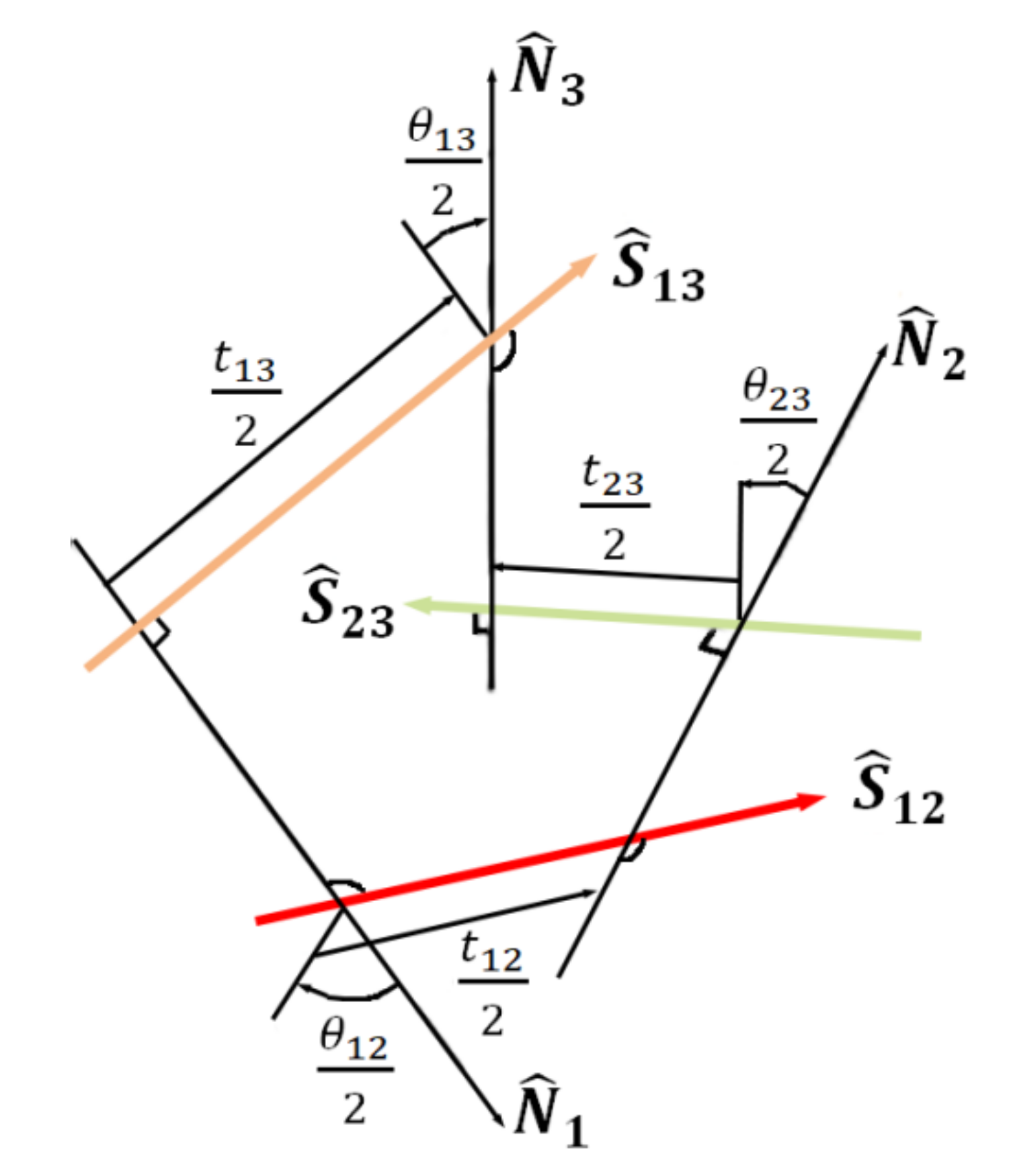
24] introduced a systematic approach based on the screw theory, in which the displacement screw was divided into two component screws. One of these is a specific screw used for displacing the specified body element, while the other is a screw used for displacing the body without affecting the specified element displacement. Incompletely specified displacement problems were investigated based on the concept of the screw triangle (see
Figure 8). When three body positions, namely
,
, and
, are specified, three corresponding screws, namely
,
, and
, exist, but only two are independent. The axes of these three screws and their normals,
,
, and
, form a spatial figure known as the screw triangle [
25,
26]. The normals and screw axes are displaced from one another by distances and angles corresponding to one-half of the screw translations,
, and one-half the screw rotations,
. For further details on the triangle screw and incompletely specified displacement screw system, the reader can refer to [
27]. The resultant twist
of two successive screw displacements
and
can be expressed as follows [
28].
where
is the screw product of
and
; the axis of
is the common perpendicular to the axes of
and
; and
and
are pure-translation screws that are parallel to the axes of
and
, respectively.
A simplified form of Equation (23), when assuming
,
, and
are small,
, and
, can be expressed as follows:
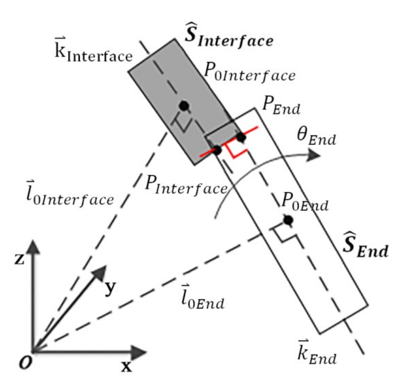
For welding axis alignment required of the pipe end, the incompletely specified displacement can be divided into two successive displacements, as illustrated in
Figure 9, as follows.
The first is a completely specified displacement (that is, position and orientation):
Position: and , where is the perpendicular foot through of the end segment axis, which indicates one unconstrained DOF.
Orientation: and , which are represented by and , respectively, where is the product of and .
The second is an unconstrained displacement that does not affect the axis alignment of the pipe end: the rotation of the pipe end around its axis is , while the unconstrained parameter is the rotation angle , which represents an additional unconstrained DOF.
In summary, the welding axis alignment model of the pipe end requires four DOFs, and can be approximately expressed using the simplified incompletely specified displacement screw system, as per Equation (24).
2.4. Solution Method
The equations set between the dimensional variation propagation and welding axis alignment models include highly nonlinear coupling. The Newton–Raphson iterative algorithm is used to solve the nonlinear equations set in this study. Based on the computation of the Jacobian matrix, the nonlinear equations set can quickly converge.
Using Equation (21), the Jacobian matrix of the dimensional variation propagation model of an adjustable pipe can be calculated in Equation (5).
where
Using Equations (16)–(19), can be represented in detail as follows:
where
(see
Figure 7), depending on the actual pose of the adjustable pipe.
3. Experimental Results and Discussions
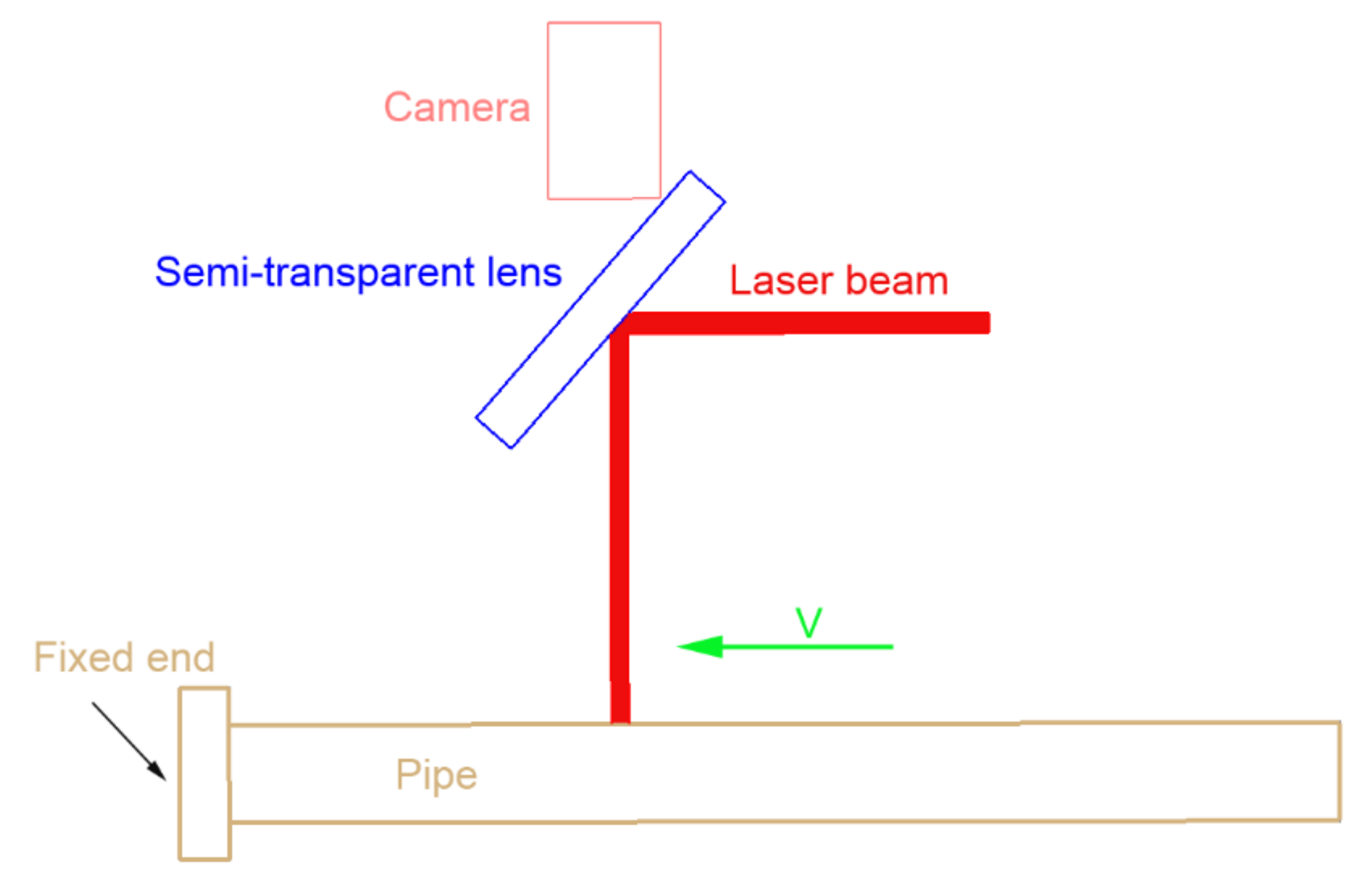
In this study, a multi-mode pulse Nd: YAG laser (Rofin StarWeld 250, Max. 250 W, 1064 nm) is used to heat and bend the pipe, as seen in
Figure 10. One end of the pipe is fixed with a triangular chuck. A high-power laser is incident on the pipe surface at a constant laser power. The triangular chuck rotates around the pipe axis with a constant scanning speed. A camera is mounted coaxially to the laser beam, and a real-time image of the bend section is captured on site.
In this experiment, the number of scans varied for different bending angles required. To avoid melting of the pipes, the laser bending experiment was carried out with constant process parameters as follows:
Laser output power (W): P = 24 W
Laser spot diameter: d = 1 mm
Scanning velocity: v = 500 mm/min
Scanning length: L = 10 mm
Scanning wrap angle: 180°
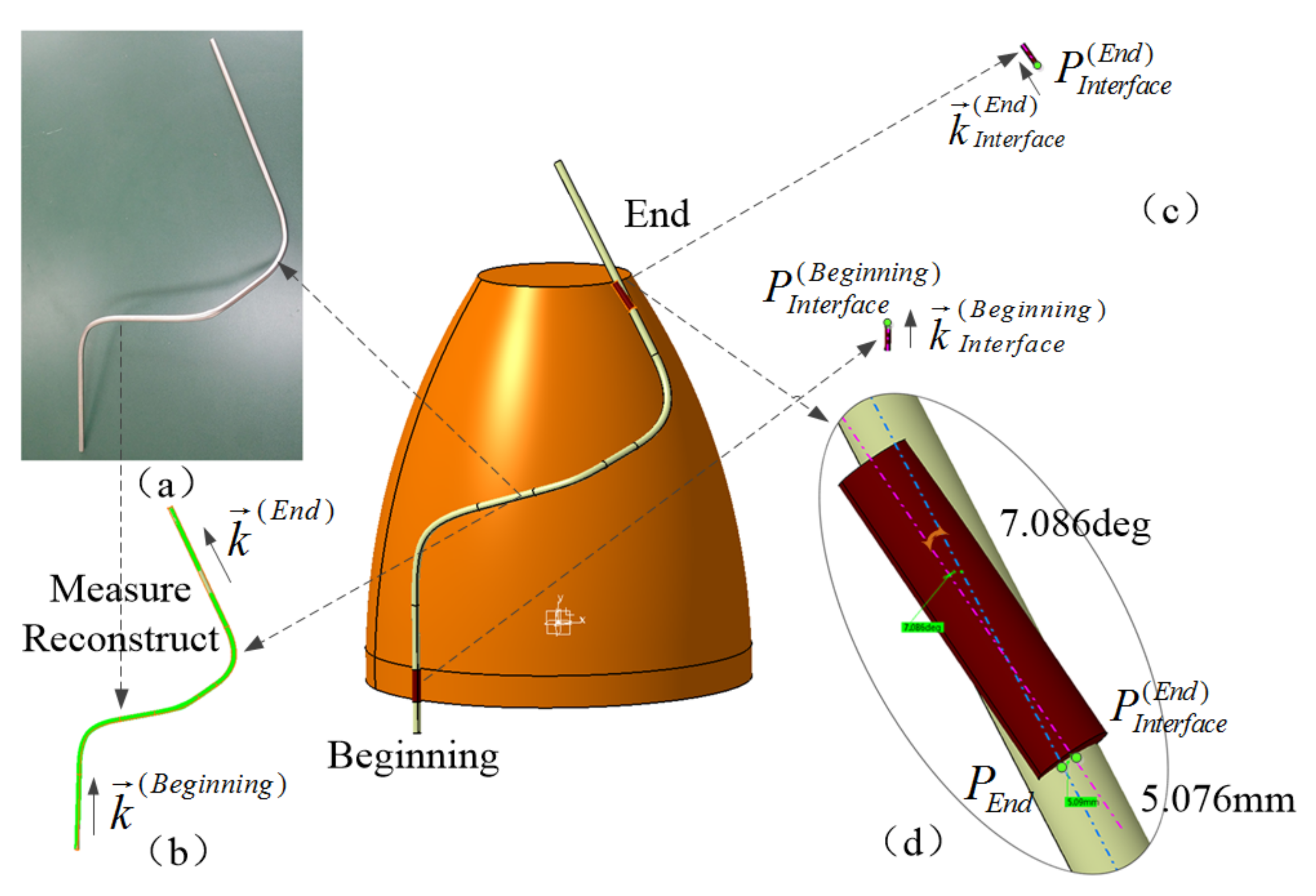
Figure 11 illustrates the initial state for the virtual assembly of an adjusted pipe. An adjustable pipe and pair of interfaces were measured by employing 3D laser scan (FARO
® Quantum), following the production process after welding, as shown in
Figure 11a. The shapes and characteristics of the adjustable pipe and interfaces were reconstructed and extracted based on the measurement data, as illustrated in
Figure 11b,c. In the current case, the existing angle deviation is 7.086°, while the existing distance deviation is 5.076 mm, as indicated in
Figure 11d. The initial poses of the adjustable pipe and interfaces are given in
Table 1.
It can be seen from Equation (21) that an adjustable pipe has five adjustable DOFs. In contrast, the welding axis alignment model of the pipe end requires four DOFs, as illustrated in
Figure 9. Owing to the higher adjustable DOF, a series of feasible calculation solutions exist that satisfy the actual geometry constraints and engineering rules, as given in
Table 2.
Figure 12 illustrates the virtual assembly following calculation of the adjustable pipe, where the feedback parameters used are from No. 5 in
Table 2. In the current case, the adjustable pipe was adjusted with respect to the corresponding interface, including the position and orientation. The residual deviation of the pipe end is only 0.0067 mm.
Figure 13 shows the final assembly by means of three adjustments approaches. The shortening length of the beginning is 4.477 mm. The rotation angle around the axis of the beginning is 1.139°. Six scans were executed for inserting the bend section by the pipe laser bending process. The bending angle obtained is 7.456°. The deviation analysis indicates that the calculation-actual contour for the adjustable pipe declined by approximately −0.836, to 0.932 mm. The residual angle deviation is 0.154°, while the residual distance deviation is 0.104 mm. The results demonstrate that the proposed adaptive control system for an adjustable pipe to compensate for production errors in rocket engine production is feasible and accurate. The poses of the adjustable pipe end and corresponding interface are provided in
Table 3.


