
A Two-Stage Transfer Regression Convolutional Neural Network for Bearing Remaining Useful Life Prediction


1
Science and Technology on Thermal Energy and Power Laboratory, Wuhan 430205, China
2
College of Intelligence and Computing, Tianjin University, Tianjin 300072, China
3
Hangzhou Yineng Electric Technology Co., Ltd., Hangzhou 310014, China
4
State Grid Zhejiang Electric Power Research Institute, Hangzhou 310014, China
*
Author to whom correspondence should be addressed.
Machines 2022, 10(5), 369; https://doi.org/10.3390/machines10050369
Submission received: 25 March 2022
/
Revised: 20 April 2022
/
Accepted: 24 April 2022
/
Published: 12 May 2022
(This article belongs to the Special Issue Fault Diagnosis and Health Management of Power Machinery)
Abstract
:Recently, deep learning techniques have been successfully used for bearing remaining useful life (RUL) prediction. However, the degradation pattern of bearings can be much different from each other, which leads to the trained model usually not being able to work well for RUL prediction of a new bearing. As a method that can adapt a model trained on source datasets to a different but relative unlabeled target dataset, transfer learning shows the potential to solve this problem. Therefore, we propose a two-stage transfer regression (TR)-based bearing RUL prediction method. Firstly, the incipient fault point (IFP) is detected by a convolutional neural network (CNN) classifier to identity the start time of degradation stage and label the training samples. Then, a transfer regression CNN with multiloss is constructed for RUL prediction, including regression loss, classification loss, maximum mean discrepancy (MMD) and regularization loss, which can not only extract fault information from fault classification loss for RUL prediction, but also minimize the probability distribution distance, thus helping the method to be trained in a domain-invariant way via the transfer regression algorithm. Finally, real data collected from run-to-failure bearing experiments are analyzed by the TR-based CNN method. The results and comparisons with state-of-the-art methods demonstrate the superiority and reliable performance of the proposed method for bearing RUL prediction.
1. Introduction
As a critical component in almost all forms of rotating machinery, the health operation of bearings has a major impact on the performance of mechanical systems [1,2,3]. The tough working environment of high temperature, high pressure and humidity will inevitably cause bearings degradation [4]. Thus, to avoid the associated economic losses and catastrophic failures, the remaining useful life (RUL) prediction of bearings plays an increasing crucial role in many industrial fields, including mining, aviation, railway and so on [5,6].
In the literature, a great variety of techniques have been proposed for RUL prediction, which coarsely include model-based methods and data-driven methods [7]. Owing to the era of big data, more and more data types and datasets are available with the development of various sensing techniques [8], which have led to the enormous development of data-driven RUL prediction methods in recent decades [9]. Instead of using failure mechanisms in model-based methods, data-driven methods rely on historical data and attempt to directly derive the degradation pattern of a machine from the data for RUL prediction [10]. In traditional data-driven RUL prediction methods, a signal processing technique is always applied firstly for feature extraction, such as statistic analysis [11], empirical mode decomposition (EMD) [12], wavelet transform [13], sparse representation [14,15] and Gaussian mixture model (GMM) [16]. Then, the extracted degradation features are used as the inputs of a regression model for RUL prediction. Machine learning methods are widely used as the prediction model, such as neural networks [17], Bayesian methods [18], support vector regression (SVR) [19] and hidden Markov model [20]. Recently, deep learning has shown its potential in fault diagnosis of mechanical systems because of its strong capacity for feature extraction, which aims to extract high-level features from raw data directly and automatically [21]. Since 2016, deep learning methods have been successfully introduced to fault diagnosis of many mechanical systems or components [22], including bearing [23], motor [21] and gearbox [24]. The research on deep-learning-based RUL prediction is relatively scarce. Deep convolutional neural network (CNN) was applied for RUL estimation of aero-engine unit prognostics. The experimental results verified the superiority of the deep CNN [25]. J. Zhu et al. proposed a multiscale CNN to keep both the local and global information synchronously, then estimated the RUL of bearings [8]. Y. Wu et al. proposed a long short-term memory (LSTM) network-based RUL prediction method. The performance improvement of the proposed method was verified by monitoring the health conditions of aircraft turbofan engines [26]. The major challenge in applying deep learning in bearing RUL prediction lies in the degradation pattern of bearings that can be much different from each other due to many complex factors, such as materials, manufacturing process and operational environment [27]. Therefore, the training data and test data for RUL prediction model obey significantly different distributions. Thus, the deep learning model trained with the vibration signals of a bearing usually cannot work well directly for RUL prediction of another bearing. In this case, transfer learning provides a good way to solve the problem [28,29]. Transfer learning aims to learn a model with better performance for the target domain by transferring the knowledge learned from the related source domain. The model constructed by knowledge transfer can reduce the requirement of large labeled samples of the target domain and obtain good generalization performance [30]. Therefore, it holds the ability to overcome the aforementioned challenge in recent data-driven RUL prediction methods. Ding et al. proposed an RUL prediction method for rolling bearing based on a deep transfer auto-encoder, which can easily determine the degradation stage of bearings under different working conditions [31]. Mao et al. proposed a transfer learning approach to improve the RUL prediction performance across different working conditions based on phase space warping (PSW), dynamic time warping (DTW), and meta-degradation information [32]. Huang et al. constructed a transfer depth-wise separable convolution recurrent network for bearing RUL prediction from the same public datasets considering different work conditions [33]. Meng et al. proposed a dynamic reweighted domain adaption method for cross-domain bearing fault diagnosis, which was verified via extensive experiments on several bearing fault diagnosis datasets [34]. However, most of the existing methods predict the RUL directly, without considering the start time of failure. Since little fault information can be found from the vibration signals under normal condition, it is important to find the start time of failure, which is called the incipient fault (IF) point in this paper.
Therefore, we propose a two-stage transfer regression (TR) CNN method for RUL prediction of an unknown bearing with the help of the historical data of training bearings. Firstly, a CNN classifier is constructed for IF point identification. Thus, the vibration data of training bearings can be labeled based on the IF point. Then, a TR CNN is proposed in this paper, which is trained by the labeled training data and used for an unknown bearing RUL prediction. The innovations of this paper are summarized as follows.
- 1.
- An end-to-end CNN classifier is firstly constructed for IF point identification, which can detect the IF point without the help of feature extractor.
- 2.
- A two-stage TR-CNN method is proposed based on transfer learning for bearing RUL prediction, which can help the method to be trained in a domain-invariant way by minimizing the probability distribution distance, namely the maximum mean discrepancy (MMD). Since the distributions of the bearing vibration datasets are usually different from each other, the proposed method is expected to be a promising method for RUL prediction.
- 3.
- Via proposing the regression loss, classification loss, MMD term and regularization term, a multiloss CNN model is constructed as the backbone architecture to extract the fault information from the fault diagnosis for RUL prediction, thus making full use of the historical data and increasing the performance of the proposed method.
- 4.
- Experimental results of the publicly available PRONOSTIA dataset [35] demonstrate the effectiveness of the proposed method.
2. Proposed Approach
2.1. Problem Description
A machinery RUL prediction system is generally composed of four stages: data acquisition, health indicator construction, IF point identification and RUL prediction [36]. In this paper, the experiment data come from the publicly available PRONOSTIA dataset, and the proposed method is constructed based on a deep learning method, which can extract features automatically without the need for the health indicator construction, so we mainly focus on the last two stages.
Firstly, since we cannot monitor the condition all the time during the bearing operation, the IF point should be determined first. Thus, the data after IF point contain the degradation information and can be used to train the prediction model. In addition, the training samples can be labeled based on the IF point.
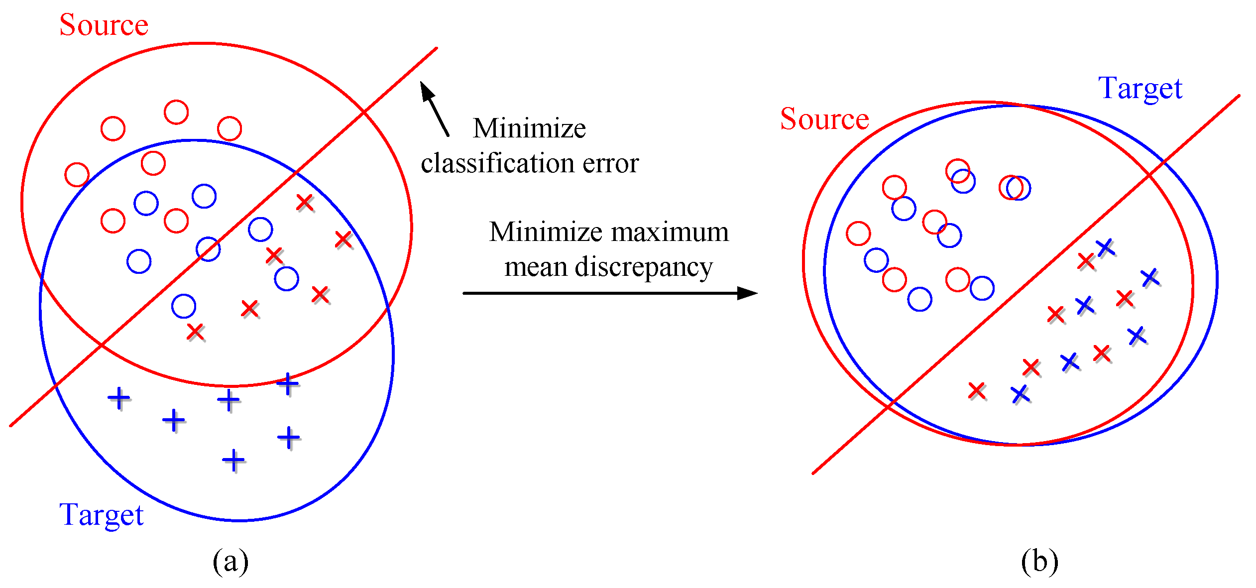
For the RUL prediction stage, let and denote the source domain and target domain, respectively. and represent the sample spaces of source domain and target domain with marginal probability distribution and , respectively. and are the data samples. Because the degradation pattern of bearings can be much different from each other due to many complex factors, the training data and test data for the prediction model are subject to substantially different data spaces and marginal distributions, namely, and , as shown in Figure 1a. The label space is defined as . In this paper, the relative RUL percentage was applied instead of the absolute RUL value, therefore, the labels of the source and target domains were the same, that is, . The goal of the transfer regression algorithm is to learn a kernel function F that satisfies and , as shown in Figure 1b. In this way, the trained regression model is also expected to work well for the RUL prediction of new bearings.
2.2. Convolutional Neural Network
The proposed RUL prediction framework was constructed based on a CNN backbone; therefore, the CNN model is briefly introduced here. As one of the most commonly used model of deep learning methods, a CNN can learn how to extract feature and recognize patterns of different tasks directly and automatically. Generally, a CNN is a multistage neural network. The former part consists of several layers, which contains the convolutional layer and the pooling layer. Classification is implemented by the latter part, in which fully connected layers are employed.
2.2.1. Convolutional Layer
The convolutional layer generates the feature maps by sliding the kernels on the input signals. Each of these kernels outputs a feature map. Then, by filtering these feature maps, the desired fault features can be extracted and rearranged according to the similarity of the embedding characteristics. By means of a series of convolutions, the desired features can be rearranged and mined by similar statistical characteristic among the feature maps. Then, a nonlinear activation function is imposed after convolution to obtain the output feature map [8]. In this paper, the ReLU function was applied as the activation function. Thus, the output feature map of the convolutional layer can be written as:
where ∗ denotes the convolution operator; and are the ith input feature map of layer and the jthe output feature map of layer l; and are the convolutional kernel and bias; is the rectified linear unit activation function, which is defined as:
2.2.2. Pooling Layer
In the pooling layer, a statistical value of a local region is calculated as the output, which can reduce the size of feature maps and increase the computational efficiency. In addition, the subsampling operation can also make the output feature maps invariant to small variance. In this paper, max-pooling was utilized:
where m is the step size of pooling and p and q are the pixel of x and y direction, respectively. c and d are the coordinate of x and y direction, respectively.
2.2.3. Fully Connected Layer
The fully connected layer is usually introduced after the feature extraction layers that consist of convolutional layers and pooling layers. A soft-max classifier is usually applied at the last layer of the CNN for classification or regression.
2.3. Incipient Fault Point Identification
IF point identification is the first task for RUL prediction, which is often detected experimentally due to the difference of failure time between machines, which can be time-consuming. Therefore, to make the RUL prediction framework more intelligent, a CNN classifier is firstly proposed to detect the IF point in this stage, which can extract the fault features automatically via the deep networks. As an end-to-end deep learning method, a CNN can detect the IF point automatically without the demand of prior knowledge, physical model or human labor.
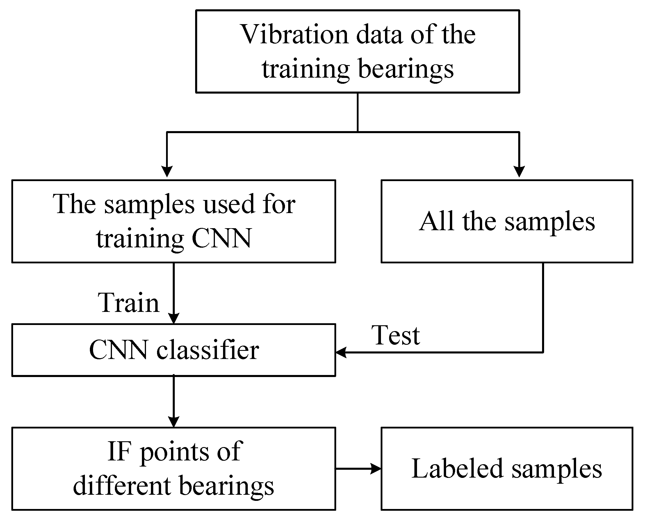
In this stage, the normal samples and the samples with obvious fault of the training bearings were labeled as 0 and 1, respectively, and used to train a CNN classification model . After obtaining the detection model , all the samples of the training bearings were used as the inputs of . When the output of changed to 1 from 0, the IF point was detected. After obtaining the IF points, all the samples of the training bearings were labeled from 0 to 1 as the relative RUL based on the IF points, for training the CNN regression model. Meanwhile, all the samples were also labeled as 0 or 1 to train the fault classification model. Thus, every sample had two labels: the first label was the relative RUL and the second label the fault type.
The flowchart of the CNN classifier for IF point identification is shown in Figure 2. In the process of RUL prediction, once the IF point of the test bearing has been detected, the vibration data can be used for RUL prediction, which is described in the next two sections.
2.4. Maximum Mean Discrepancy
MMD is a nonparametric distance to estimate the discrepancy between two distributions [37]. Specifically, MMD introduces a reproducing kernel Hilbert space (RKHS) for discrepancy determination. For example, for the samples with two different distributions, the mean values of function f can be obtained by looking for the continuous function f. Then, the mean discrepancy to function f can be obtained by calculating the difference between the two mean values. MMD aims to find a function f that can maximize the mean discrepancy. Thus, MMD can be used as a criterion to estimate whether the two distributions are the same or not. If the MMD of these two distributions is small enough, then they can be regarded as the same distribution and vice versa.
Let F be a continuous function library. For the data from and , the MMD is defined as:
where means the value on the right of the equal sign is equal to the value on the left. f is the nonlinear transformation from the original feature space to the RKHS.
In the case where and are independent identically distributed (IID), and there are n and m samples in and , respectively, the MMD can be calculated as:
where represents the ith sample from the source domain and represents the jth sample from the target domain.
Then, the characteristic kernels guide the RKHS via a kernel mean embedding of the distribution. Thus, the MMD based on the kernel mean embedding is defined as:
where is a universal RKHS and is the characteristic kernel.
2.5. Transfer Regression Method
Although transfer learning provides a promising tool to realize the domain adaption and improve the performance of the target learner by transferring the knowledge extracted from the source domain, it is mostly used for classification tasks. Therefore, a transfer regression (TR) method is proposed based on transfer learning theory for bearing RUL prediction. Considering there may exist a synergistic effect between fault diagnosis and RUL prediction, a multiloss transfer network was constructed in this stage as the backbone architecture. This multiloss structure can learn a shared feature between parallel tasks, which provides an inductive transfer way to use the domain-specific data characteristic of different but related tasks [38]. For example, two simple independent neural networks for fault diagnosis and RUL prediction were constructed, respectively. The parameters of the two neural networks should be optimized separately, which increases the computational requirement. Moreover, because they are trained separately, the feature maps cannot be shared, that is, the information of one task cannot be used in another task. However, as we all know, RUL is related to the degradation condition, and a failure can lead to the bearing degradation. As a result, much information used for fault diagnosis can also be utilized for the RUL prediction task [39]. Therefore, a multiloss network was constructed in this paper to extract the fault information from fault diagnosis, then used for the RUL prediction.
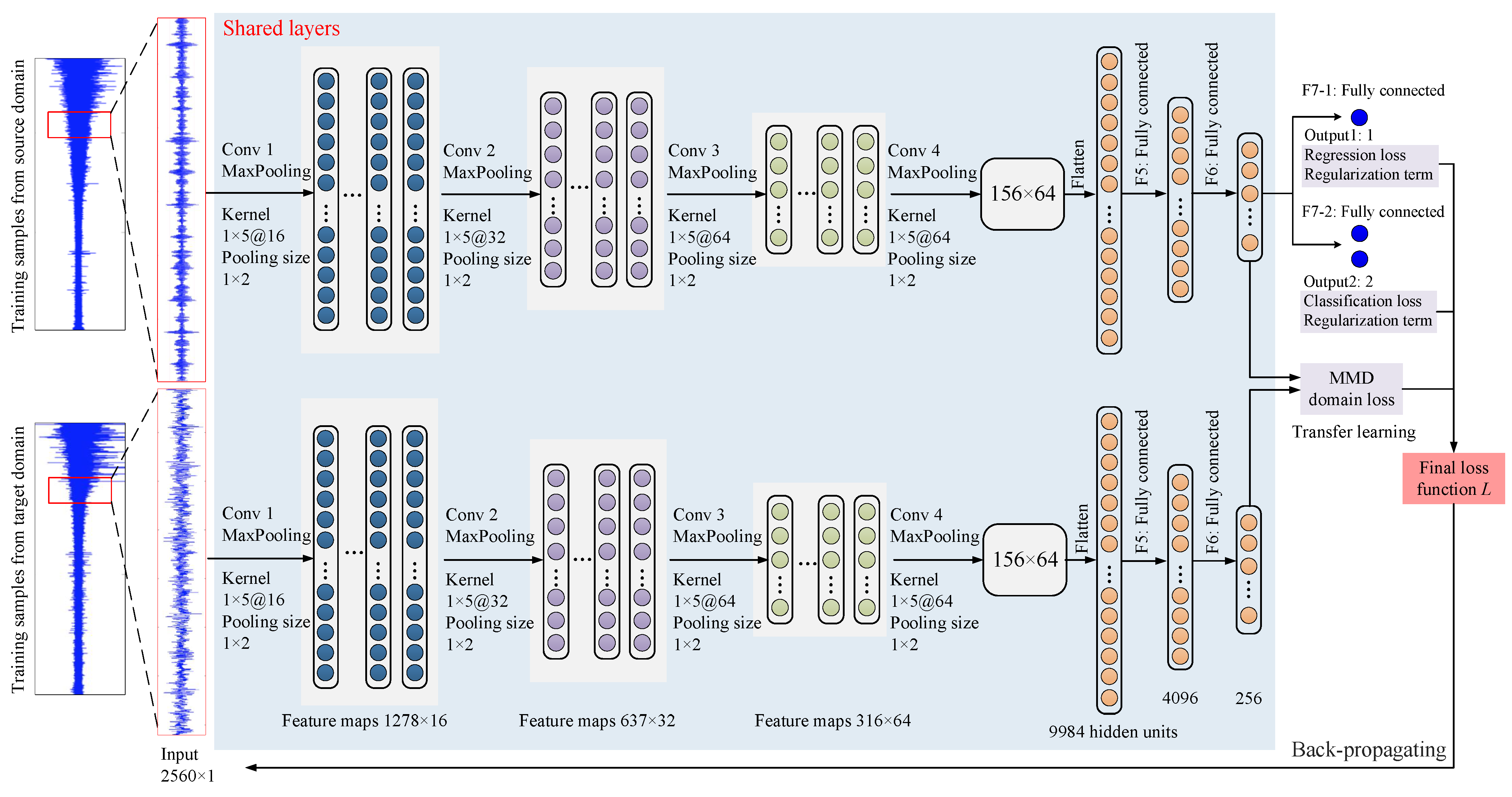
Specifically, the flowchart of the TR-CNN prediction method is graphically illustrated in Figure 3. During the training process, the vibration signals from the two domains were cut into segments as the samples. After the IF point identification step, the labels of the training dataset from the source domain for both fault classification and RUL prediction were obtained. Thus, the training samples from the source domain with corresponding labels, as well as the unlabeled samples from the target domain were used to train the multiloss model. The label of the first task was the relative RUL obtained based on the IF point; the label of second task was the fault type. Therefore, there were two loss functions needed to be optimized: the regression loss and the classification loss. In addition, to adapt the differences between the source domain dataset and target domain dataset, the MMD term should also be minimized. As a result, the final loss function consisted of four parts: regression loss, classification loss, MMD term and regularization term.
2.5.1. Regression Loss
The objective of this task is to fit the degradation process with nonlinear functions. Firstly, after the IF points detection, the samples before the IF points were labeled with 1, and the samples after the IF points were labeled with the healthy percentages:
where is the label at time ; is the total time of the test; is the start time of IF; and is the current time.
Then, the samples were labeled with the health percentage and input to the multiloss CNN model. For RUL prediction, the selected loss function was the mean squared error.
where is the ith label, and is the ith input. n is the number of samples.
2.5.2. Classification Loss
In this task, the vibration datasets of the training bearings were labeled as 0 or 1 based on IF points, where 0 represents the normal bearing and 1 represents the faulty bearing. Then, the labeled training samples were used as the inputs of the multiloss model. For this task, the selected loss function was the cross-entropy:
where is the target distribution and is the estimated distribution.
2.5.3. MMD Term
The transfer layer was placed after the fully connected layer . In the transfer layer, the discrepancy metric of labeled samples was realized by the MMD term:
where represents the input of the transfer layer in the source domain and represents the input of the transfer layer in the target domain.
2.5.4. Regularization Term
The regularization term (also called weight decay term) is a commonly used loss, which can decrease the magnitude of the weights and help prevent overfitting. The regularization term is defined as:
where m is the number of layers in the network; is the size of a hidden unit in layer l; is the weight that connect the ith unit in layer l and the jth unit in layer .
2.5.5. Final Loss Function
Therefore, the final loss function of the TR-based RUL prediction model consisted of four parts:
- 1.
- The regression loss ;
- 2.
- The classification loss of CNN model ;
- 3.
- The MMD term for domain adaption between the source domain and target domain.
- 4.
- The regularization term .
Thus, the final loss function was given as follows:
where , and controlled the trade-off among these four loss functions and were determined empirically. b is the bias parameter.
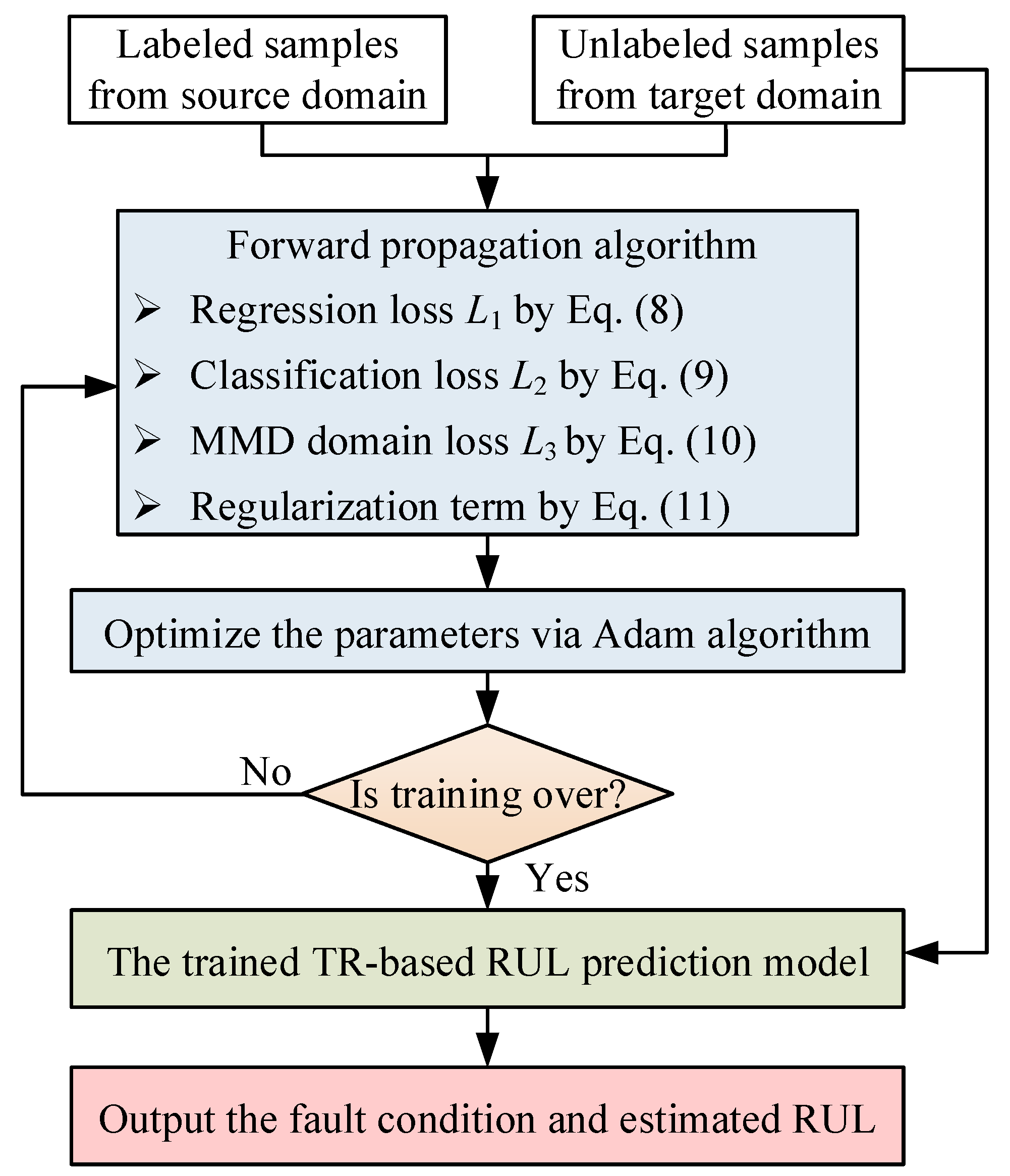
After the training was over, the TR-based RUL prediction model took test data as input to calculate the fault condition and the estimated RUL.
2.6. Training Process
During the training process of the TR-based RUL prediction model, the Adam optimization algorithm was applied to minimize the loss function in Equation (12) [40]. Let represent the gradient vector at time t of the loss function , the estimations of the first moment (the mean) and second moment (the uncentered variance) of the gradients can be described as:
where is the control weight; and are exponential decay rate of first order and second order, respectively; ; and are set with bias correction:
Then, the parameters can be updated:
where is the parameter set; is a constant with small positive value used to avoid the division for zero. Thus, the parameters can be optimized more stably.
The flowchart of the proposed RUL prediction framework is presented in Figure 4.
3. Experiments, Results and Discussion
3.1. Experimental Setup and Data Description
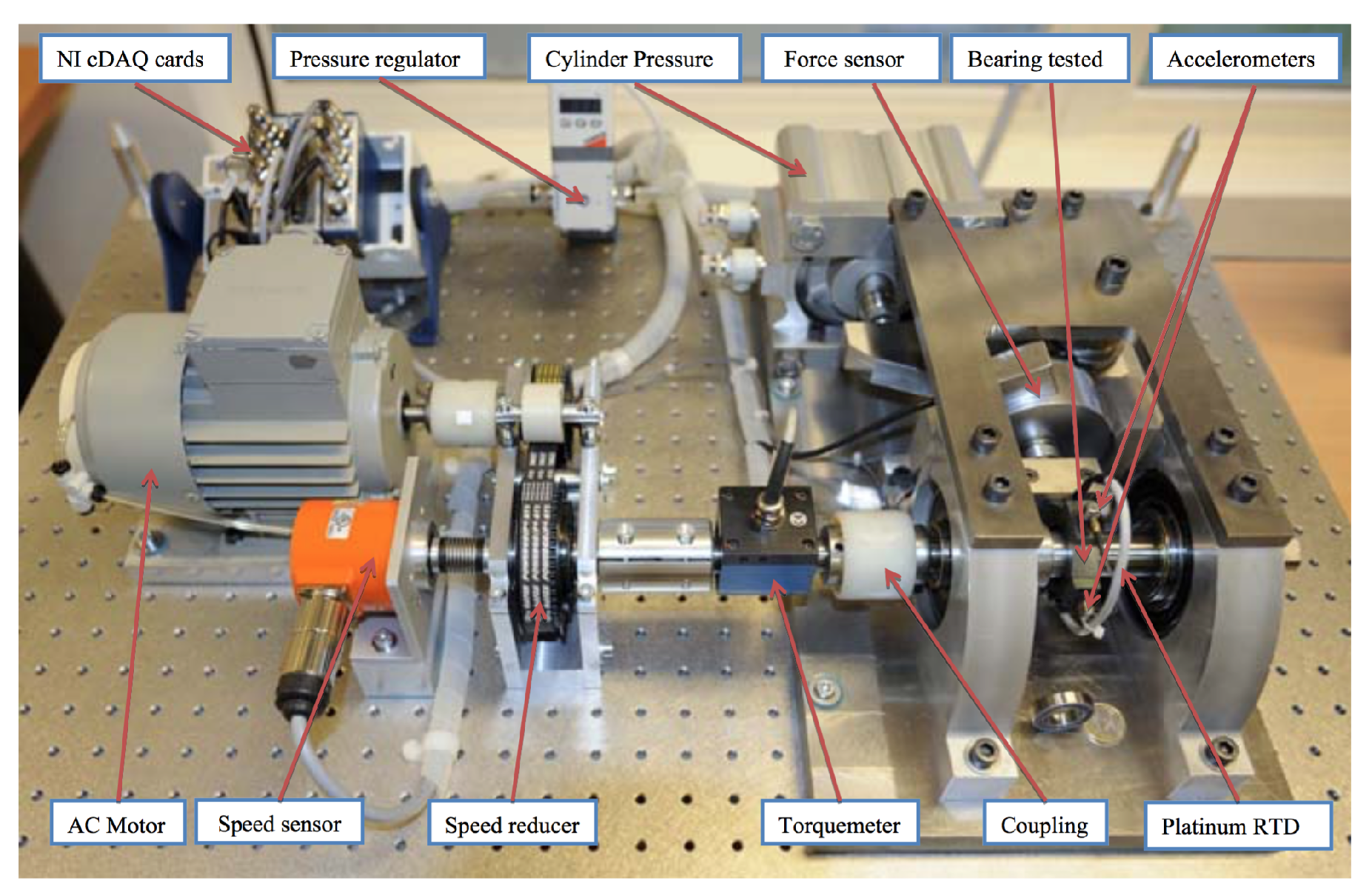
The dataset came from the PRONOSTIA experimental platform in the IEEE PHM 2012 Data Challenge [35]. Figure 5 shows the overview of the experimental platform. The main objective of PRONOSTIA is to provide real data related to accelerated degradation of bearings performed under constant and/or variable operating conditions, which are online controlled. The operating conditions are characterized by two sensors: a rotating speed sensor and a force sensor. In the PRONOSTIA platform, the bearing’s health monitoring is ensured by gathering online two types of signals: temperature and vibration (horizontal and vertical accelerometers). The experiment was conducted under three conditions. In condition 1, the radial load force was 4000 N and the shaft speed was 1800 r/min; in condition 2, the radial load force was 4200 N and the shaft speed was 1650 r/min; in condition 3, the radial load force was increased to 5000 N and the shaft speed was 1500 r/min. The vibration sensors collected 0.1 s vibration signals every 10 s with a sampling frequency of 25.6 kHz. In this paper, each segment with 2560 points (0.1 s) was regarded as a sample.
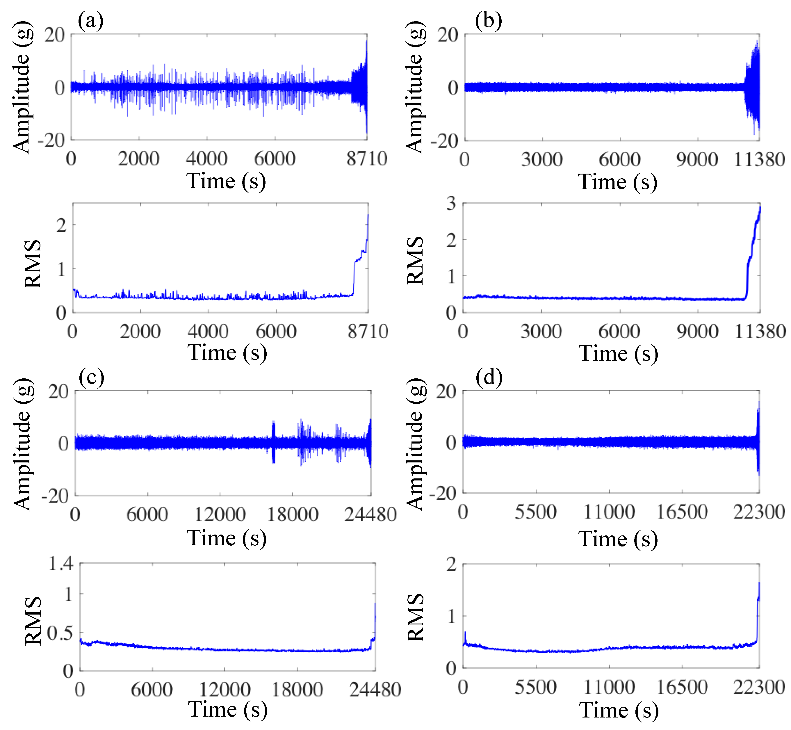
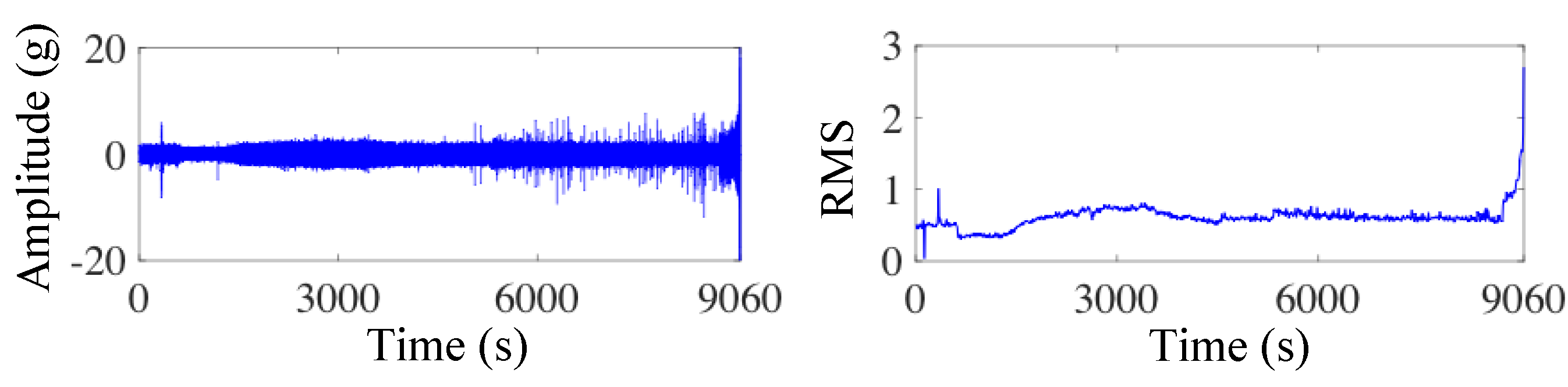
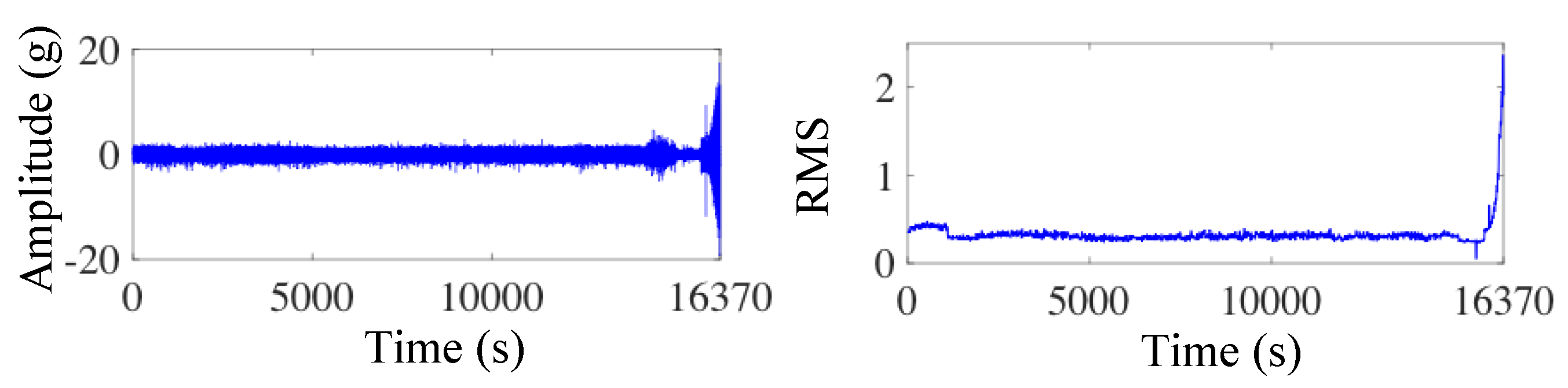
To verify the effectiveness of the proposed method and its transfer ability between different conditions, two cases were analyzed. The vibration signals of four tests in condition 1 were selected as the source domain datasets, as shown in Figure 6. In case 1, one test in condition 2 was used as the target domain dataset. The vibration waveforms and the corresponding RMS are shown in Figure 7. In case 2, one test in condition 3 was used as the target domain dataset, as shown in Figure 8. Table 1 describes the datasets in the source domain and target domain in detail. The sample number of each dataset is shown in Table 2.
Firstly, CNN was trained on the training samples to extract the features from the vibration signal as the input of the RUL prediction model. Then, the IF points of different training datasets in source domain were identified by CNN. The degradation times of the four source domain datasets were identified to be 8250 s, 10,820 s, 24,110 s and 22,070 s, respectively. The source samples were labeled by the IF points. In this step, the sample corresponds to two labels: the classification label (0 or 1) and the regression label (the relative RUL from 0 to 1). That is, the sample becomes . The target domain datasets were unlabeled because the test dataset cannot be labeled in practical applications.
3.2. Case 1
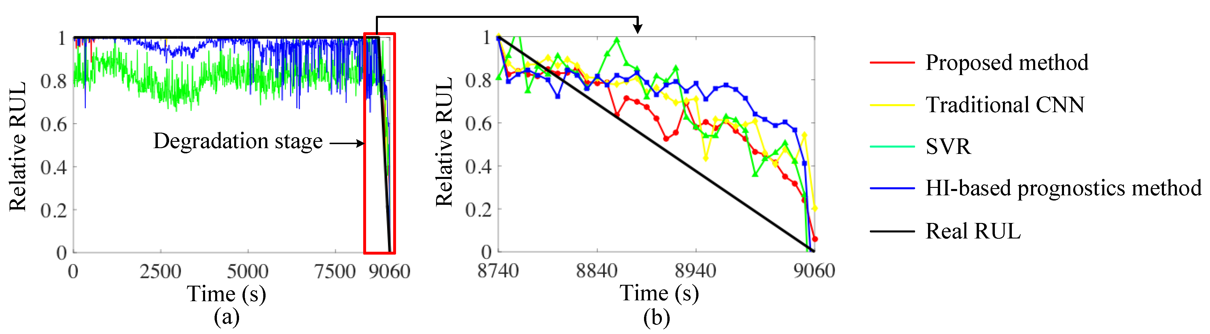
In this case, one test dataset in condition 2 was used as the target dataset. Since the operational condition in the target domain was different from the source domain, the proposed TR-based prediction method was introduced for the RUL prediction. The proposed method was implemented in Python 3.5 based on a NVDIA GeForce GTX 1060 GPU. The parameters of the Adam optimization method were selected as: . The learning rate was selected as 0.001, the weight decay was set to 0 and the batch size was set to 32. There were 50 epochs in this experiment. The prediction results are shown in Figure 9. In order to further demonstrate the effectiveness of the proposed method, three state-of-the-art methods, including a traditional CNN, an SVR and a health index (HI)-based prediction method, were introduced to the same data as baseline methods for comparison. In order to verify the improvement of the prediction accuracy via multiloss architecture and transfer learning, the architecture of the traditional CNN was the same as that of the proposed method except that there was no F7-2 output and MMD domain loss in the last layer. The inputs of the SVR were set to be eleven time and frequency domain features, including RMS, kurtosis, mean and so on. Furthermore, the detail of the HI-based prediction method is illustrated in [41]. The results of these three methods are also drawn in Figure 9 for easier comparison.
It can be observed from Figure 9 that during the normal process from 0 s, the SVR does not perform as good as the other methods. The predicted relative RUL of the normal stage should be 1. The results of the SVR (the green line) show shocks around 0.8. The HI-based method also shows some shocks, but better than the SVR. The traditional CNN and the proposed method can provide a more accurate prediction result in this stage. Furthermore, during the degradation process, the HI-based method shows a higher variance than other methods. The prediction results of the two-stage TR-CNN are closer to those of the real RUL. Therefore, it can be concluded that the main limitation of the SVR is that it cannot detect if the bearing begins to degrade or not based on the historical data. Furthermore, the main drawback of the HI-based method is the low prediction accuracy during the degradation process.
For a better illustration and numerical comparison, the mean square error (MSE) of the two-stage TR-CNN and the three baseline methods was calculated as an estimation index, as shown in Table 3. Matching with the prediction results in Figure 9, the MSE of the SVR is highest in the full life cycle, which is mainly caused by the prediction error during the normal stage. Furthermore, the MSE of the HI-based method is highest during the degradation stage. It can also be seen that the MSE of the two-stage TR-CNN is smallest both during full life cycle and degradation stage, which demonstrates that the proposed method not only can detect if the current bearing is faulty or not based on the collected signal, but that it also provides a more accurate predicted relative RUL.
3.3. Case 2
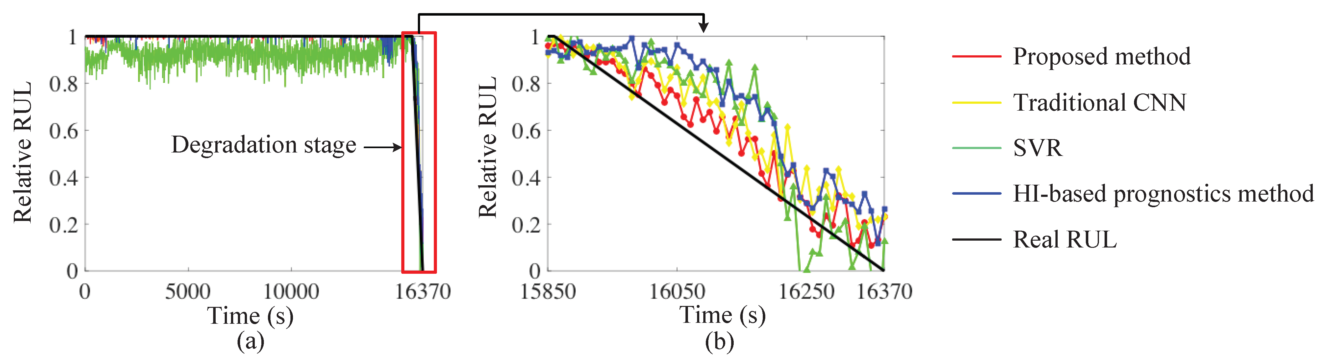
In this case, one test dataset of condition 3 was used as the unlabeled target dataset. Then, the proposed method, as well as three comparison methods were employed to predict the relative RUL of the target dataset. The prediction results are shown in Figure 10.
It can be found from Figure 10a that the SVR (green line) is still not good at estimating the relative RUL during the normal stage, which is similar to case 1. From the local enlarged area in Figure 10b, it can be seen that both the SVR and HI-based prediction method (blue line) show higher variance because the prediction results of these two methods are farther from the real relative RUL (black line). This is because the degradation pattern of bearings can be very different due to many factors, such as the changeable operational conditions, processing techniques and so on, which can lead to the instability of features, thus influencing the prediction performance of feature-based methods. The traditional CNN (yellow line) performs better than SVR and HI-based method because the CNN can automatically learn high feature hierarchies via its deep architecture without the help of a feature extractor, thus avoiding the influence of unstable features. It can also be found that the prediction results of the two-stage TR-CNN (red line) are closest to the real RUL both during the full life cycle and degradation stage, which verifies the effectiveness of the proposed method.
In this case, MSE was also used as the estimation index, which is shown in Table 4. It can be seen that the proposed TR-based RUL prediction method shows the lowest MSE both in full life cycle and degradation stage. This is because the proposed method was constructed based on a multiloss CNN backbone, which made it not only possess the superiority of CNN, but also able to learn fault features from fault classification, which can be used for RUL prediction. More than that, transfer learning can bridge the discrepancy between the dataset from different domains, thus learn transferable features and provide a more accurate estimated RUL results.
4. Conclusions
The main challenge for bearing RUL prediction is the difference in the degradation process between two bearings. Inspired by transfer learning, this paper proposed a TR-based RUL prediction method for bearing RUL prediction. A multiloss CNN was constructed as the backbone to make full use of historical data by extracting fault features from fault classification and then using them for RUL prediction. The application of a transfer learning algorithm also enabled the proposed method to learn transferable features between different domains. The effectiveness and transfer ability of the two-stage TR-CNN were verified by two experiments under different conditions. The experimental results illustrated that the two-stage TR-CNN was able to predict the RUL of the bearing tested under different conditions. The comparisons with state-of-the-art RUL prediction methods also illustrated the superiority of the proposed method. However, since the proposed method was constructed based on deep learning, more training datasets can improve the prediction performance. Because there are several parameters still needed to be determined manually and empirically, a more adaptive approach for the parameter selection shall be developed in the future.
Author Contributions
Conceptualization, X.L. and K.Z.; methodology, X.L.; software, R.L.; validation, R.L. and K.Z.; formal analysis, W.L.; investigation, Y.F.; resources, R.L.; data curation, Y.F.; writing—original draft preparation, X.L.; writing—review and editing, K.Z.; visualization, Y.F.; supervision, R.L.; project administration, Y.F.; funding acquisition, X.L. All authors have read and agreed to the published version of the manuscript.
Funding
This research received no external funding.
Institutional Review Board Statement
Not applicable.
Informed Consent Statement
Not applicable.
Data Availability Statement
Data available on request due to privacy/ethical restrictions.
Conflicts of Interest
The authors declare no conflict of interest.
References
- Yuan, H.; Wu, N.; Chen, X.; Wang, Y. Fault diagnosis of rolling bearing based on shift invariant sparse feature and optimized support vector machine. Machines 2021, 9, 98. [Google Scholar] [CrossRef]
- Nguyen, V.C.; Hoang, D.T.; Tran, X.T.; Van, M.; Kang, H.J. A Bearing Fault Diagnosis Method Using Multi-Branch Deep Neural Network. Machines 2021, 9, 345. [Google Scholar] [CrossRef]
- Cheng, F.; Qu, L.; Qiao, W.; Hao, L. Enhanced Particle Filtering for Bearing Remaining Useful Life Prediction of Wind Turbine Drivetrain Gearboxes. IEEE Trans. Ind. Electron. 2019, 66, 4738–4748. [Google Scholar] [CrossRef]
- Peng, Y.; Wang, Y.; Zi, Y. Switching State-Space Degradation Model With Recursive Filter/Smoother for Prognostics of Remaining Useful Life. IEEE Trans. Ind. Inform. 2019, 15, 822–832. [Google Scholar] [CrossRef]
- Wang, B.; Lei, Y.; Li, N.; Wang, W. Multiscale Convolutional Attention Network for Predicting Remaining Useful Life of Machinery. IEEE Trans. Ind. Electron. 2021, 68, 7496–7504. [Google Scholar] [CrossRef]
- Xiahou, T.; Zeng, Z.; Liu, Y. Remaining Useful Life Prediction by Fusing Expert Knowledge and Condition Monitoring Information. IEEE Trans. Ind. Inform. 2021, 17, 2653–2663. [Google Scholar] [CrossRef]
- Lei, Y.; Li, N.; Gontarz, S.; Lin, J.; Radkowski, S.; Dybala, J. A model-based method for remaining useful life prediction of machinery. IEEE Trans. Reliab. 2016, 65, 1314–1326. [Google Scholar] [CrossRef]
- Zhu, J.; Chen, N.; Peng, W. Estimation of Bearing Remaining Useful Life Based on Multiscale Convolutional Neural Network. IEEE Trans. Ind. Electron. 2019, 66, 3208–3216. [Google Scholar] [CrossRef]
- Zhao, H.; Liu, H.; Jin, Y.; Dang, X.; Deng, W. Feature Extraction for Data-Driven Remaining Useful Life Prediction of Rolling Bearings. IEEE Trans. Instrum. Meas. 2021, 70, 1–10. [Google Scholar] [CrossRef]
- Gao, Y.; Wen, Y.; Wu, J. A Neural Network-Based Joint Prognostic Model for Data Fusion and Remaining Useful Life Prediction. IEEE Trans. Neural Netw. Learn. Syst. 2021, 32, 117–127. [Google Scholar] [CrossRef]
- Tian, Z. An artificial neural network method for remaining useful life prediction of equipment subject to condition monitoring. J. Intell. Manuf. 2012, 23, 227–237. [Google Scholar] [CrossRef]
- Lei, Y.; Lin, J.; He, Z.; Zuo, M.J. A review on empirical mode decomposition in fault diagnosis of rotating machinery. Mech. Syst. Signal Process. 2013, 35, 108–126. [Google Scholar] [CrossRef]
- Yan, R.; Gao, R.X.; Chen, X. Wavelets for fault diagnosis of rotary machines: A review with applications. Signal Process. 2014, 96, 1–15. [Google Scholar] [CrossRef]
- Yang, B.; Liu, R.; Chen, X. Fault diagnosis for a wind turbine generator bearing via sparse representation and shift-invariant K-SVD. IEEE Trans. Ind. Inform. 2017, 13, 1321–1331. [Google Scholar] [CrossRef]
- Yang, B.; Liu, R.; Chen, X. Sparse Time-Frequency Representation for Incipient Fault Diagnosis of Wind Turbine Drive Train. IEEE Trans. Instrum. Meas. 2018, 67, 2616–2627. [Google Scholar] [CrossRef]
- Yu, J. Bearing performance degradation assessment using locality preserving projections and Gaussian mixture models. Mech. Syst. Signal Process. 2011, 25, 2573–2588. [Google Scholar] [CrossRef]
- Tian, Z.; Wong, L.; Safaei, N. A neural network approach for remaining useful life prediction utilizing both failure and suspension histories. Mech. Syst. Signal Process. 2010, 24, 1542–1555. [Google Scholar] [CrossRef]
- Chen, C.; Zhang, B.; Vachtsevanos, G. Prediction of machine health condition using neuro-fuzzy and Bayesian algorithms. IEEE Trans. Instrum. Meas. 2012, 61, 297–306. [Google Scholar] [CrossRef]
- Khelif, R.; Chebel-Morello, B.; Malinowski, S.; Laajili, E.; Fnaiech, F.; Zerhouni, N. Direct remaining useful life estimation based on support vector regression. IEEE Trans. Ind. Electron. 2017, 64, 2276–2285. [Google Scholar] [CrossRef]
- Dong, M.; He, D. A segmental hidden semi-Markov model (HSMM)-based diagnostics and prognostics framework and methodology. Mech. Syst. Signal Process. 2007, 21, 2248–2266. [Google Scholar] [CrossRef]
- Shao, S.; Yan, R.; Lu, Y.; Wang, P.; Gao, R.X. DCNN-Based Multi-Signal Induction Motor Fault Diagnosis. IEEE Trans. Instrum. Meas. 2020, 69, 2658–2669. [Google Scholar] [CrossRef]
- Jia, F.; Lei, Y.; Lin, J.; Zhou, X.; Lu, N. Deep neural networks: A promising tool for fault characteristic mining and intelligent diagnosis of rotating machinery with massive data. Mech. Syst. Signal Process. 2016, 72, 303–315. [Google Scholar] [CrossRef]
- Wang, X.; Wang, T.; Ming, A.; Zhang, W.; Li, A.; Chu, F. Cross-Operating Condition Degradation Knowledge Learning for Remaining Useful Life Estimation of Bearings. IEEE Trans. Instrum. Meas. 2021, 70, 1–11. [Google Scholar] [CrossRef]
- Jiang, G.; He, H.; Yan, J.; Xie, P. Multiscale Convolutional Neural Networks for Fault Diagnosis of Wind Turbine Gearbox. IEEE Trans. Ind. Electron. 2019, 66, 3196–3207. [Google Scholar] [CrossRef]
- Yang, B.; Liu, R.; Zio, E. Remaining Useful Life Prediction Based on a Double-Convolutional Neural Network Architecture. IEEE Trans. Ind. Electron. 2019, 66, 9521–9530. [Google Scholar] [CrossRef]
- Wu, Y.; Yuan, M.; Dong, S.; Lin, L.; Liu, Y. Remaining useful life estimation of engineered systems using vanilla LSTM neural networks. Neurocomputing 2018, 275, 167–179. [Google Scholar] [CrossRef]
- Miao, M.; Yu, J. A Deep Domain Adaptative Network for Remaining Useful Life Prediction of Machines Under Different Working Conditions and Fault Modes. IEEE Trans. Instrum. Meas. 2021, 70, 1–14. [Google Scholar] [CrossRef]
- Zhuang, F.; Qi, Z.; Duan, K.; Xi, D.; Zhu, Y.; Zhu, H.; Xiong, H.; He, Q. A Comprehensive Survey on Transfer Learning. Proc. IEEE 2021, 109, 43–76. [Google Scholar] [CrossRef]
- Yang, B.; Lei, Y.; Jia, F.; Xing, S. An intelligent fault diagnosis approach based on transfer learning from laboratory bearings to locomotive bearings. Mech. Syst. Signal Process. 2019, 122, 692–706. [Google Scholar] [CrossRef]
- Zhu, J.; Chen, N.; Shen, C. A New Deep Transfer Learning Method for Bearing Fault Diagnosis Under Different Working Conditions. IEEE Sens. J. 2020, 20, 8394–8402. [Google Scholar] [CrossRef]
- Ding, Y.; Ding, P.; Jia, M. A Novel Remaining Useful Life Prediction Method of Rolling Bearings Based on Deep Transfer Auto-Encoder. IEEE Trans. Instrum. Meas. 2021, 70, 1–12. [Google Scholar] [CrossRef]
- Mao, W.; He, J.; Sun, B.; Wang, L. Prediction of Bearings Remaining Useful Life Across Working Conditions Based on Transfer Learning and Time Series Clustering. IEEE Access 2021, 9, 135285–135303. [Google Scholar] [CrossRef]
- Huang, G.; Zhang, Y.; Ou, J. Transfer remaining useful life estimation of bearing using depth-wise separable convolution recurrent network. Measurement 2021, 176, 109090. [Google Scholar] [CrossRef]
- Meng, Y.; Xuan, J.; Xu, L.; Liu, J. Dynamic Reweighted Domain Adaption for Cross-Domain Bearing Fault Diagnosis. Machines 2022, 10, 245. [Google Scholar] [CrossRef]
- Nectoux, P.; Gouriveau, R.; Medjaher, K.; Ramasso, E.; Chebel-Morello, B.; Zerhouni, N.; Varnier, C. PRONOSTIA: An experimental platform for bearings accelerated degradation tests. In Proceedings of the IEEE International Conference on Prognostics and Health Management, PHM’12, IEEE Catalog Number: CPF12PHM-CDR, Denver, CO, USA, 18–21 June 2012; pp. 1–8. [Google Scholar]
- Lei, Y.; Li, N.; Guo, L.; Li, N.; Yan, T.; Lin, J. Machinery health prognostics: A systematic review from data acquisition to RUL prediction. Mech. Syst. Signal Process. 2018, 104, 799–834. [Google Scholar] [CrossRef]
- Borgwardt, K.M.; Gretton, A.; Rasch, M.J.; Kriegel, H.P.; Schölkopf, B.; Smola, A.J. Integrating structured biological data by kernel maximum mean discrepancy. Bioinformatics 2006, 22, e49–e57. [Google Scholar] [CrossRef] [Green Version]
- Caruana, R. Multitask learning. Mach. Learn. 1997, 28, 41–75. [Google Scholar] [CrossRef]
- Liu, R.; Yang, B.; Hauptmann, A.G. Simultaneous Bearing Fault Recognition and Remaining Useful Life Prediction Using Joint Loss Convolutional Neural Network. IEEE Trans. Ind. Inform. 2019, 16, 87–96. [Google Scholar] [CrossRef]
- Kingma, D.P.; Ba, J. Adam: A method for stochastic optimization. arXiv 2014, arXiv:1412.6980. [Google Scholar]
- Yang, F.; Habibullah, M.S.; Zhang, T.; Xu, Z.; Lim, P.; Nadarajan, S. Health index-based prognostics for remaining useful life predictions in electrical machines. IEEE Trans. Ind. Electron. 2016, 63, 2633–2644. [Google Scholar] [CrossRef]
Figure 1.
(a) The classifier cannot work well on both biased datasets. (b) The classifier can be transferred to the target domain by minimizing the MMD.
Figure 1.
(a) The classifier cannot work well on both biased datasets. (b) The classifier can be transferred to the target domain by minimizing the MMD.

Figure 2.
The flowchart of the CNN for IF point identification.

Figure 3.
Architecture of the proposed TR method.

Figure 4.
Flowchart of the proposed TR-based RUL prediction framework.

Figure 5.
PRONOSTIA experimental platform.

Figure 6.
Vibration signals and RMS of (a) bearing ; (b) bearing ; (c) bearing ; (d) bearing .

Figure 7.
Vibration signals and RMS of bearing .

Figure 8.
Vibration signals and RMS of bearing .

Figure 9.
(a) RUL prediction results of the proposed method, traditional CNN method, SVR and HI-based prognostics method; and (b) their enlargement. The red line represents the result of the proposed method; the yellow line represents the traditional CNN method; the green line represents the SVR result; the blue line represents the HI-based method and the black line represents the real RUL.

Figure 10.
(a) RUL prediction results of the proposed method, traditional CNN method, SVR and HI-based prognostics method and (b) their enlargement.
Figure 10.
(a) RUL prediction results of the proposed method, traditional CNN method, SVR and HI-based prognostics method and (b) their enlargement.


Table 1.
Description of datasets.
| Source Domain | Target Domain Dataset of Case 1 | Target Domain Dataset of Case 2 | |
|---|---|---|---|
| Conditions | Condition 1 | Condition 2 | Condition 3 |
| Datasets | 1_1, 1_2, 1_3, 1_4 | 2_1 | 3_1 |
Table 2.
Sample number of each dataset.
| Dataset | 1_1 | 1_2 | 1_3 | 1_4 | 2_1 | 3_1 |
|---|---|---|---|---|---|---|
| Samples | 871 | 1138 | 2448 | 2230 | 906 | 1637 |
Table 3.
MSE of the proposed method, CNN, SVR and the HI-based method in case 1.
| Proposed Method | CNN | SVR | HI-Based Method | |
|---|---|---|---|---|
| Full life cycle | 0.0014 | 0.0023 | 0.381 | 0.0080 |
| Degradation stage | 0.0350 | 0.0617 | 0.0810 | 0.1007 |
Table 4.
MSE of the proposed method, CNN, SVR and the HI-based method in case 2.
| Proposed Method | CNN | SVR | HI-Based Method | |
|---|---|---|---|---|
| Full life cycle | 0.0005 | 0.0015 | 0.0150 | 0.0031 |
| Degradation stage | 0.0105 | 0.0258 | 0.0413 | 0.0503 |
Publisher’s Note: MDPI stays neutral with regard to jurisdictional claims in published maps and institutional affiliations. |
© 2022 by the authors. Licensee MDPI, Basel, Switzerland. This article is an open access article distributed under the terms and conditions of the Creative Commons Attribution (CC BY) license (https://creativecommons.org/licenses/by/4.0/).
Share and Cite
MDPI and ACS Style
Li, X.; Zhang, K.; Li, W.; Feng, Y.; Liu, R. A Two-Stage Transfer Regression Convolutional Neural Network for Bearing Remaining Useful Life Prediction. Machines 2022, 10, 369. https://doi.org/10.3390/machines10050369
AMA Style
Li X, Zhang K, Li W, Feng Y, Liu R. A Two-Stage Transfer Regression Convolutional Neural Network for Bearing Remaining Useful Life Prediction. Machines. 2022; 10(5):369. https://doi.org/10.3390/machines10050369
Chicago/Turabian StyleLi, Xianling, Kai Zhang, Weijun Li, Yi Feng, and Ruonan Liu. 2022. "A Two-Stage Transfer Regression Convolutional Neural Network for Bearing Remaining Useful Life Prediction" Machines 10, no. 5: 369. https://doi.org/10.3390/machines10050369
Note that from the first issue of 2016, this journal uses article numbers instead of page numbers. See further details here.