Imbalanced Fault Diagnosis of Rolling Bearing Using Data Synthesis Based on Multi-Resolution Fusion Generative Adversarial Networks

Abstract

Fault diagnosis of industrial bearings plays an invaluable role in the health monitoring of rotating machinery. In practice, there is far more normal data than faulty data, so the data usually exhibit a highly skewed class distribution. Algorithms developed using unbalanced datasets will suffer from severe model bias, reducing the accuracy and stability of the classification algorithm. To address these issues, a novel Multi-resolution Fusion Generative Adversarial Network (MFGAN) is proposed for the imbalanced fault diagnosis of rolling bearings via data augmentation. In the data-generation process, the improved feature transfer-based generator receives normal data as input to better learn the fault features, mapping the normal data into fault data space instead of random data space. A multi-scale ensemble discriminator architecture is designed to replace original single discriminator structure in the discriminative process, and multi-scale features are learned via ensemble discriminators. Finally, the proposed framework is validated on the public bearing dataset from Case Western Reserve University (CWRU), and experimental results show the superiority of our method.

1. Introduction

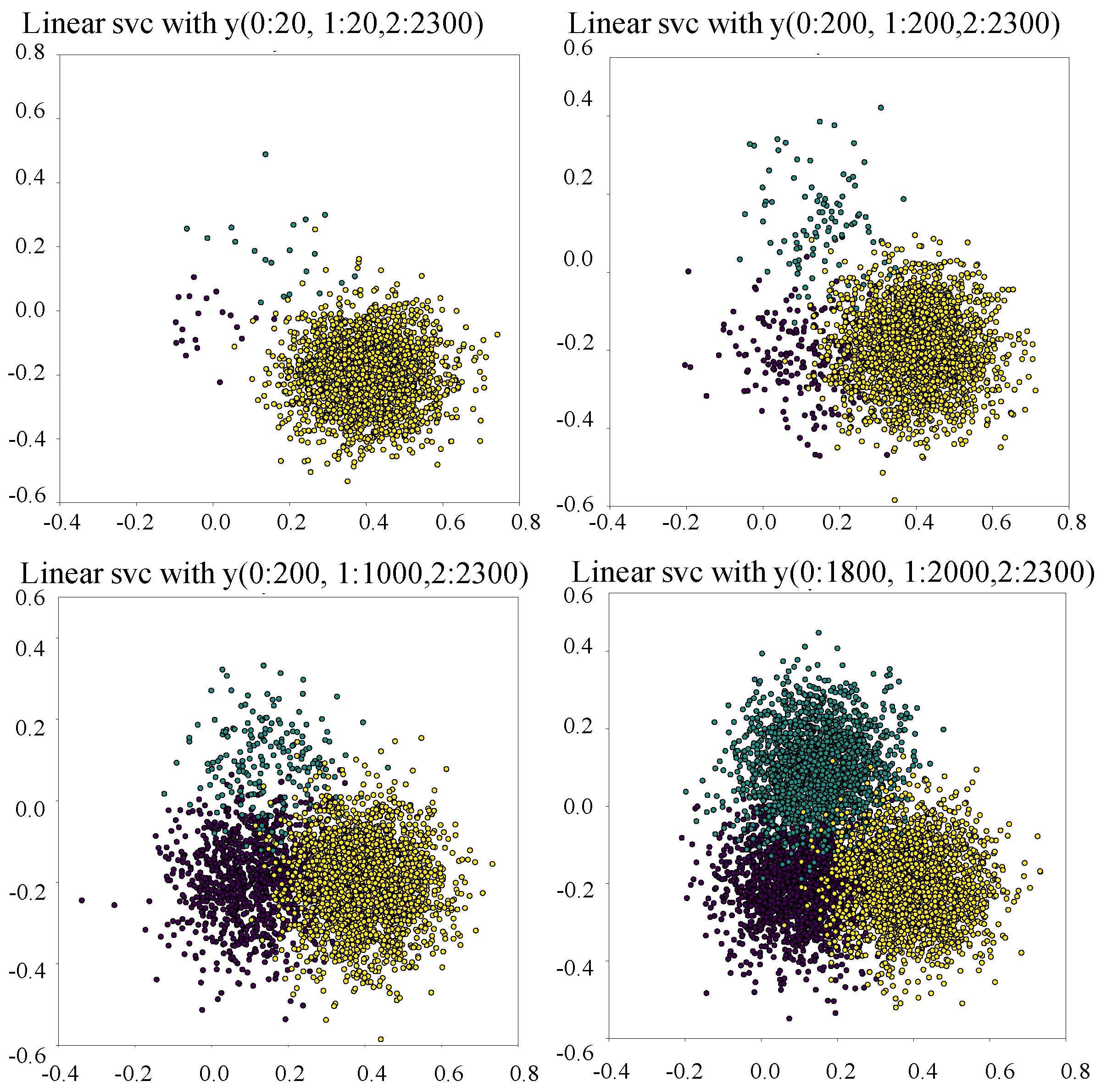
Rolling bearings are the most widely used and important component of machinery and equipment, and are also the general fault unit of industrial rotating machinery. Rolling bearings are generally composed of four parts: inner ring, outer ring, rolling body and cage. The inner ring in the bearing is generally paired to the shaft and follows this shaft to perform rotational movement. The outer ring is generally assembled to the bearing seat and is used to support the steel ball. The rolling body rolls within the bearing, and its shape, size and number directly affect the performance and service life of the bearing. Bearings are designed, manufactured, installed, operated and maintained in such a way that various factors can lead to the damage or fault of the bearing. At the same time, due to continuous operation under high intensity and harsh conditions, faults of rolling bearings are inevitable and unforeseen faults can lead to very long production downtimes and losses, causing damage to machinery may undoubtedly having catastrophic consequences. Timely and reliable fault diagnosis of rolling bearings is therefore very important [1]. Fault-prediction methods are generally divided into model-driven fault diagnosis and data-driven fault diagnosis [2]. Model-based fault diagnosis techniques require strong a priori knowledge to determine the mathematical model of the system object. In many practical problems, it is difficult to build mathematical models of complex components or systems. It is also difficult to identify suitable predictive models for sets of historical fault data or statistics that are triggered by many different signals. The practical application and effectiveness of model-based fault prediction techniques is therefore limited by the relative complexity of equipment fault modes and fault mechanisms. Data-based fault-prediction techniques do not require a priori knowledge, such as mathematical models of the object systems and expert experience. It also has better feature extraction capabilities, non-linear modelling capabilities and more powerful computational capabilities. Through the analytical processing and modelling of historical data, the implicit information is mined for diagnostic operations. Data-based fault prediction has become a more practical approach to fault prediction and is growing rapidly. With technological breakthroughs in data acquisition systems, large amounts of industrial data are readily available, which provides the basis for data-driven classification algorithms. Data is collected using monitoring systems to analyze the operating status of mechanical equipment and to carry out fault diagnosis. Fault diagnosis is one of the typical applications of data-driven methods in industry and has been a hot topic of research [3]. To date, a large number of effective classification algorithms have been applied to industrial equipment fault diagnosis problems [4,5]. In fact, few fault data can be collected, while the amount of available normal data is very huge. As a result, the data tends to show a highly skewed distribution of categories [6], i.e., most instances belong to the normal category, while the different types of fault categories contain only a small number of instances. Due to the lack of sufficient data, the classifier is unable to describe the sparse instances and therefore it is difficult to classify these sparse instances effectively. In the case of SVM, for example, the final learned classification boundaries tend to favor the majority class, leading to the problem of classification boundary bias. As can be seen from Figure 1, the boundary bias gradually increases as the dataset becomes more unbalanced, leading to a significant drop in the final classification performance. So, almost all methods for fault diagnosis of unbalanced datasets tend to be biased towards the normal class and less accurate for the fault class [7].

In order to resist the negative impact of imbalanced data on the algorithm, researchers have conducted a series of exploratory experiments [8,9]. The first alternative method is re-sampling, the idea of which is to over-sample a minority class or under-sample a majority class in order to balance their number ratio. For instance, Gu et al. [10] applied Gaussian noise to a minority class of instances to create extrapolations, and then created linear interpolation between these extrapolations to enrich the minority class of instances. However, over-sampling can easily lead to overfitting and noise introduction, and under-sampling may lose important information of the data [11]. The second alternative method is cost-sensitive learning, which assigns higher misclassification costs to the minority classes than to the majority. Feng et al. [12] proposed a Cost-sensitive Feature selection General Vector Machine algorithm to handle the imbalanced classification problem, setting different cost weights to different classes of instances. However, in most cases, cost weights cannot be obtained from data or specified by experts, which limits the application of cost-sensitive learning based methods [13].

Recently, a new alternative method for data augmentation would be to use Generative Adversarial Networks (GANs) [14]. GANs have now become one of the major paradigms for image generation [15], speech synthesis [16], and text generation [17]. This is because GANs can generate instances that are almost indistinguishable from real ones. In general, GANs consists of two sub-networks, a Generator and Discriminator. The Generator maps the noise sampled from a preset distribution space to the instance in data space. At the same time, the Discriminator is used to judge whether an instance is coming from the data space or the Generator. The training is a game process, in which the generation ability and discrimination ability of GANs will be improved alternately until the Nash equilibrium is reached [14]. However, the application of GANs to vibration signals generation tasks in industrial intelligent diagnosis has seen relatively limited success so far [18]. Moreover, there are some problems, i.e., mode collapse, unstable training, and slow convergence, in the training process of GANs [19].

Based on the above analysis, how to make use of the data distribution of a few fault data to generate similar and diverse synthetic instances adaptively is the key to improve the effect of imbalanced fault diagnosis. This article proposes a novel data augmentation method based MFGAN architecture to eliminate data imbalance. MFGAN introduces feature transfer into GANs to reduce the difficulty of data augmentation and make full use of the normal data. The generator maps the normal data into the fault data space to accomplish fault data augmentation. Moreover, it can be embedded into any generation model of similar tasks, so it has good generality. Meanwhile, we extend a single discriminator to multi-scale ensemble discriminator architecture (MSED) to help MFGAN learn data features on multiple time scales to ensure more stable training and the high authenticity of the synthetic data. Finally, we apply the proposed data augmentation method to public rolling bearing datasets, and the experimental results show that the proposed method is superior. Our contributions are as follows:

(1)

A novel Multi-resolution Fusion Generative Adversarial Network (MFGAN) is proposed for fault diagnosis on unbalanced datasets. The discriminator of MFGAN is composed of three sub-discriminators, the input of each sub-discriminator is the vibration signal at different subsampling frequencies, and then the output results of the sub-discriminator are fused. MFGAN can obtain more stable training and produce high-quality synthetic data.

(2)

A data-enhancement method based on feature transfer and MFGAN is proposed. Specifically, we sample the input from the normal data space and then map it to the fault data space via MFGAN to obtain rich fault data, which can be used to remove data imbalances. The method reduces the difficulty of data augmentation, improves the quality of the synthetic data and can be embedded in a generative model for any similar task with good generality.

(3)

MFGAN is evaluated quantitatively and qualitatively through a large number of experiments, and can produce higher-quality fault data and improve the accuracy of fault diagnosis. The algorithms in the paper can be replicated using open-source code available on GitHub.

2. Related Work

2.1. Re-Sampling Method

Generally, the re-sampling method is to over-sample a minority class or under-sample a majority class in order to balance their number ratio. For instance, Le et al. [20] use evolutionary-based approaches and treat under-sampling as a binary optimization problem that determines which instances in majority class are removed. Liu et al. [21] propose an under-sampling method based on information granules of majority class instances to capture the essence of them. Synthetic Minority Over-sampling Technology (SMOTE) [22] is one of the most widely used methods. It adds random deviation to the K-nearest neighbor of minority class instances to generate new instances. However, SMOTE has two problems: (1) the number of neighboring instances is a hyper-parameter, so it is difficult to obtain in advance; (2) instances generated by the minority class instances at the edge of distribution will blur the boundary between the majority class and the minority class, which is not conducive to classification. Subsequently, many improved algorithms were proposed to solve the above problems of SMOTE, i.e., MSMOTE [23], borderline-SMOTE [24], SMOTE-Bagging [25], SMOTE-CSELM [26]. However, these methods still fail to understand the underlying distribution of real data and may produce incorrect instances.

2.2. Cost-Sensitive Learning

Cost-sensitive learning allocates different error classification costs to the minority and majority class to avoid the model making decisions in favor of majority class, thus improving the classification performance of imbalanced classification. The core of cost-sensitive learning is to find the optimal cost by minimizing the total classification error cost of training instances [27]. In general, cost-sensitive learning assigns higher cost to the minority class [28]. In the past decade, various cost-sensitive learning algorithms have been proposed to cope with the problem of imbalanced data. For example, Cheng et al. [29] proposed a Cost-Sensitive Large margin Distribution Machine (CS-LDM) to improve the accuracy of minority class by introducing cost-sensitive margin mean and cost-sensitive penalty. Ghazikhani et al. [30] combined cost-sensitive learning with Neural Networks and proposed two kinds of online classifiers to solve the problem of concept drift and imbalance data. Datta et al. [31] develop Near-Bayesian Support Vector Machine (NBSVM), an improved version of SVM to reduce Bayes error in imbalanced data classification, which combines decision boundary shift with cost-sensitive learning. However, cost-sensitive learning does not increase the number of minority class instances, and the risk of overfitting still exists in the model.

2.3. Generative Adversarial Networks

Generative Adversarial Networks (GANs) proposed by Goodfellow [14] has become a popular deep generation model, which can approximate the distribution of various data. The optimization objective function of vanilla GANs is shown in Formula (1).

$$mi{n}_{G}ma{x}_D E_{x\sim P_x\left(x\right)}\left[logD\left(x\right)\right]+E_{z\sim P_z\left(z\right)}\left[log\left(1-D\left(G\left(z\right)\right)\right)\right]$$

(1)

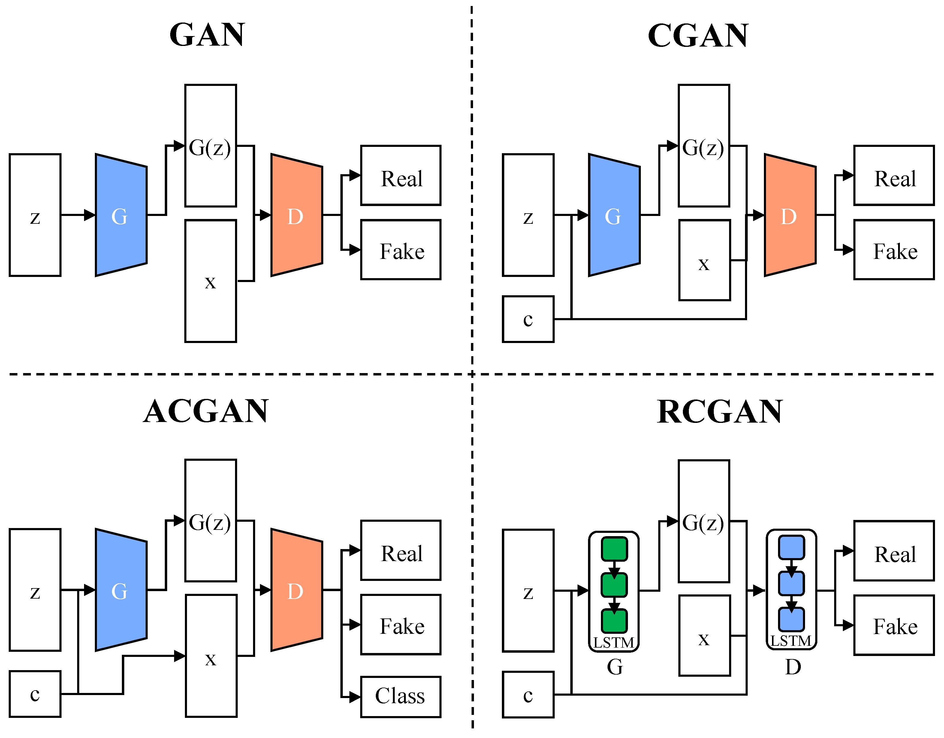
Because the data-generation process of vanilla GANs is completely random, it is impossible to generate the specified instances, which limits the practical application of vanilla GANs. A natural improvement is to add conditional information to vanilla GANs to generate specific instances. Based on this idea, researchers have proposed Conditional GANs (CGAN) [32] and Auxiliary Classifier GANs (ACGAN) [33]. Zheng et al. [34] proposed a dual-discriminator conditional generative adversarial network (D2CGANs), an improved version of CGAN, to improve the quality of rolling bearing data generation for rotating machinery. Xu et al. [35] improved ACGAN and proposed FairGAN+, which includes a generator, an auxiliary classifier and three discriminators. Erol et al. [36] use ACGAN to generate synthetic radar Micro-Doppler signatures adapted to different environments, so as to reduce the human cost of acquiring radar signals. To enable GANs to extract time-dependent characteristics and generate time series, Yu et al. [37] proposed Sequence Generative Adversarial Nets (SeqGAN), combined with Monte Carlo search, to realize the generation and evaluation of discrete sequences. Lee et al. [38] proposed a novel application of SeqGAN, which are the creating of polyphonic musical sequences. Hyland et al. [39] proposed Recurrent Conditional GANs (RCGAN) based on Long Short-Term Memory networks (LSTM). Figure 2 illustrates the framework of vanilla GAN and its variants.

3. Model Development

3.1. Overview

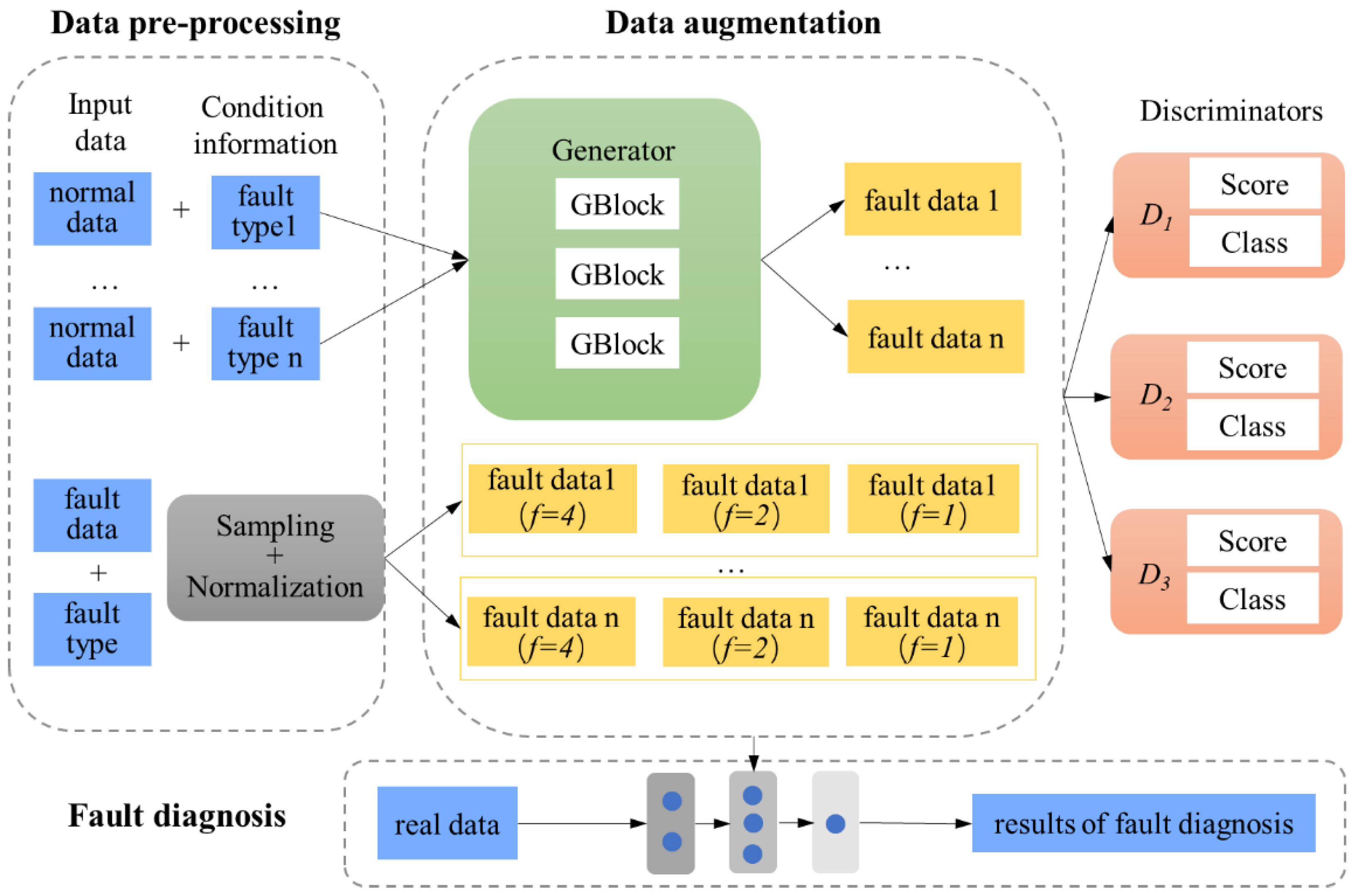
MFGAN consists of one generator G and three sub-discriminators (D₁, D₂ and D₃). Based on the condition information c, G maps the normal data to different types of fault data. The condition information c is associated with the labels of the fault data. Each sub-discriminant extracts features from different inputs at a specific sampling frequency in order to allow the total discriminant D to focus on data at different time scales. Then, we combine the outputs of all the sub-discriminators to get the output of D. The whole framework of MFGAN involves three main components, including data pre-processing, data augmentation, and fault diagnosis, which is shown in Figure 3. The following details the network structure of generator G and MSED.

3.2. Generator Architecture

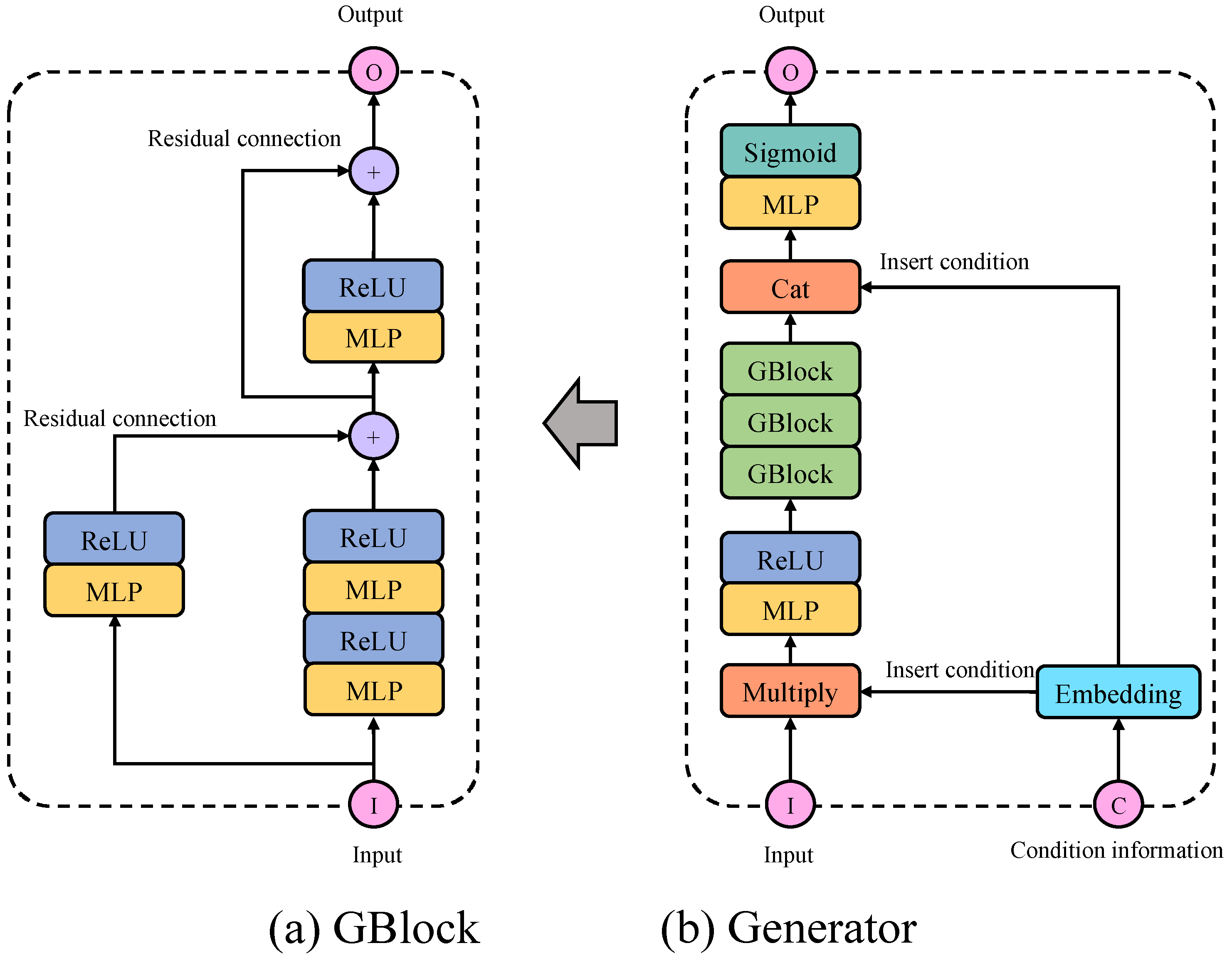
The architecture of generator G is shown in Figure 4. The input to G is a sequence of normal data and condition information c according to fault type, and its output is the fault data. There are three GBlocks in G (shown in Figure 4a), each of which is a stack of two residual blocks. Each GBlock contains two residual connections, the first of which doubles the dimension of the input and matches the dimension of the output of the main path. The second residual connection is to simply add the input of the block to the output. So, when a tensor goes into a GBlock, its dimension is doubled. Condition information (original label) c works in G in two ways after passing through the embedding layer. The first way is to multiply the conditional information c directly with the input, and the second way is to merge the c with the output of the third GBlock. The final MLP (Multilayer Perceptron) layer with Sigmoid activation produces a fault bearing data associated with c.

The time series modeling by GANs is prone to mode collapse, because the features of time series are not as rich as those of natural images. In other words, it is difficult for MFGAN to learn the distribution of all types of fault data. In order to alleviate the above problem, we construct the loss function of G based on the Model Seeking regular term. Mao et al. [40] propose to maximize the ratio of the distance between generation data and latent vectors, which encourages G to generate dissimilar data during training. In this way, G can explore the fault data space, and enhance the chances of generating instances from different modes. The calculation of Model Seeking regular term is shown in Formula (2).

$$L_{ms}=ma{x}_G\left(\frac{d_I\left(G\left(c,z_1\right),G\left(c,z_2\right)\right)}{d_z\left(z_1,z_2\right)}\right)$$

(2)

where, d_I and d_z both represent distance measurements, and c represents the condition information, z₁ and z₂ represent the noise. The smaller the value of L_ms, the more serious the mode collapse is. We make the modification to Formula (2), because the input of MFGAN is normal data rather than noise z. The modified calculation formula is shown in Formula (3).

$$L_{ms}^{\star }=ma{x}_G\left(\frac{d\left(G\left(c,x_{n1}\right),G\left(c,x_{n2}\right)\right)}{d\left(x_{n1},x_{n2}\right)}\right)$$

(3)

where, x_n1 and x_n2 represent normal data, and c represents the condition information. We set d as Euclidean distance in this article.

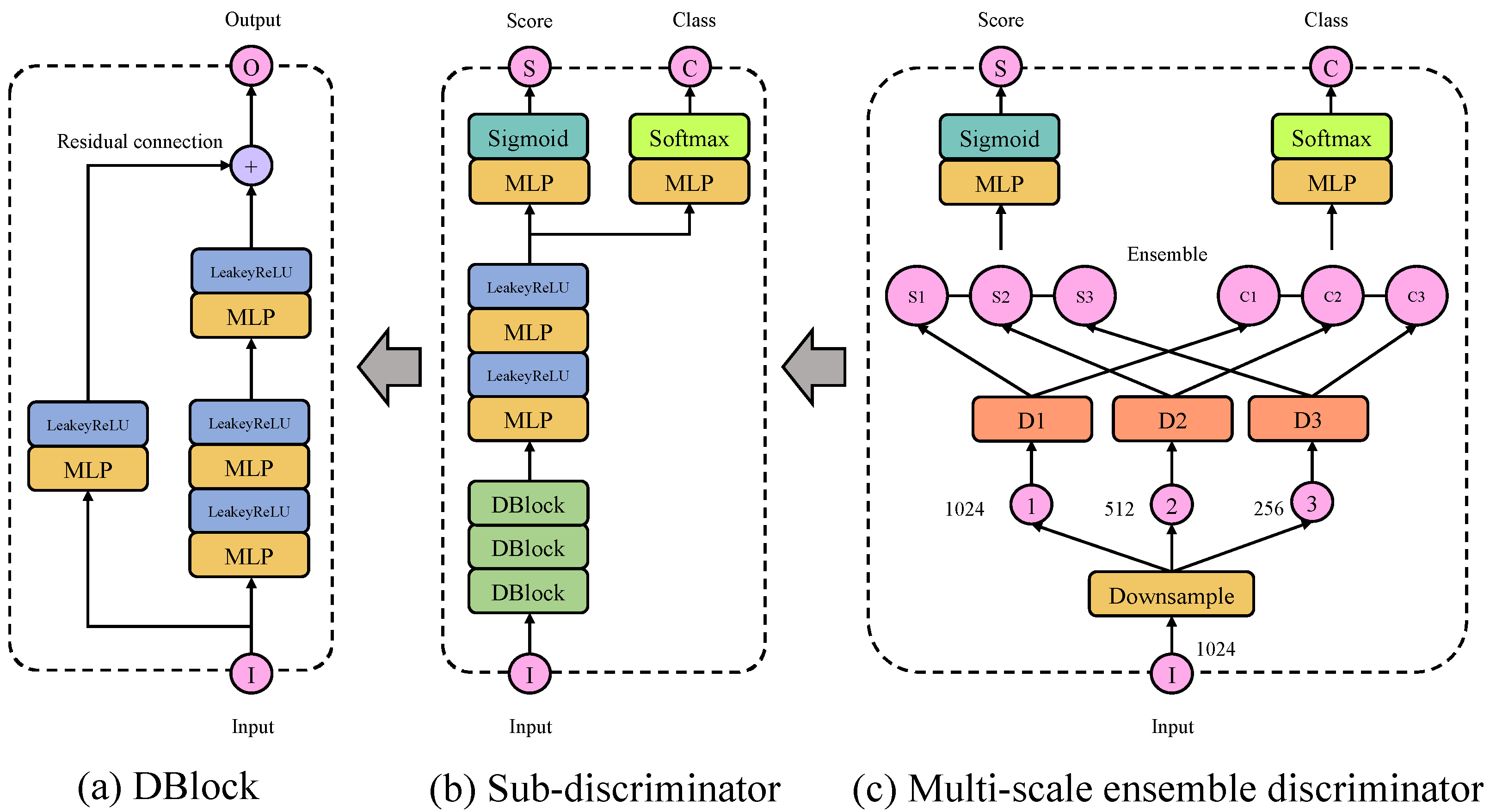
3.3. Multi-Scale Ensemble Discriminator Architecture

Instead of a vanilla single discriminator, we use Multi-scale Ensemble Discriminator (MSED) (shown as Figure 5c) to screen the authenticity of bearing signals at different time scales (sampling frequency) and classify. The MSED consists of three sub-discriminators (D₁, D₂ and D₃), and the input of which is fault data as different sampling frequencies f. In this article, we set f = [4, 2, 1], which means that the input is sub-sampled four times, two times, and then one time. Each sub-discriminator outputs a score S and a category C, where S represents whether the likelihood that the input is real and C represents the predicted category. This output is the same as that of ACGAN. There are three DBlocks in each sub-discriminator, as shown in Figure 4b. DBlock contains one residual connection and halves the dimension of the input (Figure 4a). Using different sampling frequencies, rather than just original fault data, has a data augmentation effect and rich features. This allows MFGAN to process time series well without using LSTM, as LSTM usually has the problem of low computational efficiency. Similar to ACGAN, MSED has two loss functions, as shown in Formulas (4) and (5).

$${ℒ}_{\mathcal{S}}=E\left[logP\left(S=real|X_{real}\right)\right]+E\left[logP\left(S=fake|X_{fake}\right)\right]$$

(4)

$${ℒ}_{\mathcal{C}}=E\left[logP\left(C=c|X_{real}\right)\right]+E\left[logP\left(C=c|X_{fake}\right)\right]$$

(5)

where, ${ℒ}_{\mathcal{S}}$ represents the authenticity of the generated data, which is calculated by the cross entropy between the judge result S and labels. ${ℒ}_{\mathcal{C}}$ represents the degree of matching between the generated data and the condition information.

3.4. Training Process of MFGAN

The algorithm for the MFGAN training process will be shown below, as shown in Algorithm 1 (Algorithm 1: MFGAN training process).

Algorithm 1: The algorithm for the MFGAN training process.

1: Input: normal data Xn, fault data Xf, fault data label c, number of fault types K, bacthsize B, learning rate of MSED ηϕ, learning rate of generator ηθ, steps k, iterations N, weights of loss functions [w1, w2, w3, w4] 2: Output: Trained generator Gθ 3: Randomly initialize parameters θ, ϕ 4: for n = 0 → N − 1 do 5:  Xn ← Shuffle(Xn) 6:  [Xf, c] ← Shuffle([Xf, l]) 7:  for i = 0 → k − 1 do 8:     [xB f,i=1, cB i=1], XB n,i=1 ← GetSample([X, c], B), GetSample(Xn, B) 9:     x’B f,i=1 ← G( xB n,,i=1, cB i=1) 10:    [S′, C′], [S, C] ← MSED(x’B f,i=1, cB i=1), MSED(xB n,,i=1, cB i=) 11:    Ld ← w1(${\displaystyle \sum }_i^B{S}^i$+${\displaystyle \sum }_i^{B}log\left(1-S{\prime }^i\right)$) + w2/B${\displaystyle \sum }_{i=0}^{B-1}{\displaystyle \sum }_{k=0}^{K}clogC$ 12:    ϕ ← ϕ − ηϕ∇ϕ(Ld) 13:    end for 14:  x’B f,i=1 ← G( xB n,,i=1, cB i=1) 15:  [S′, C′]← MSED(x’B f,i=1, cB i=1) 16:  LG ← w3${\displaystyle \sum }_i^{B}log\left(1-S{\prime }^i\right)$) + w2/B${\displaystyle \sum }_{i=0}^{B-1}{\displaystyle \sum }_{k=0}^{K}clogC$+ w4${ℒ}_{\mathcal{S}}$* 17:  θ ← θ − ηθ∇θ(LG) 18:  if n % 50 == 0 and n > 0 then 19:     ηϕ ← ηϕ/2 20:     ηθ ← ηθ/2 21:  end if 22: end for

4. Experimental Methodology

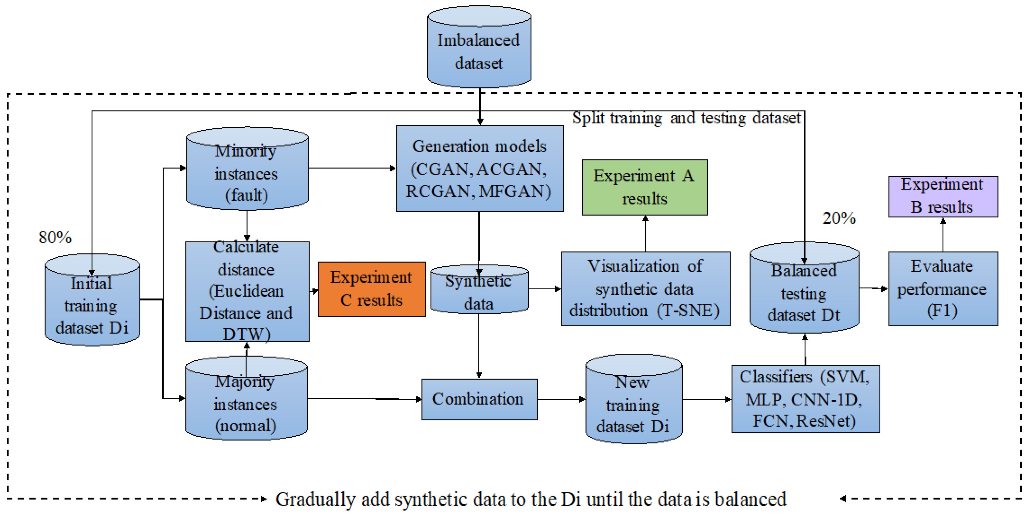
As a data-enhancement method, MFGAN can improve the performance of classification problems with unbalanced data by expanding the number of minority classes. Three experiments are conducted in this section, firstly, the quality of the synthetic data is assessed qualitatively by means of an algorithm commonly used for non-linear downscaling and data visualization, i.e., experiment A; next, the proposed model is embedded in different classifiers and compared with state-of-the-art generative models, including CGAN [32], ACGAN [33], and RCGAN [39], to quantitatively evaluate the performance and generality of MFGAN, i.e., experiment B; and finally, multiple metrics validate the effectiveness of the input feature transfer strategy, i.e., experiment C. A general flowchart of the three sets of evaluation experiments for each dataset is shown in Figure 6.

4.1. Benchmark Dataset

In order to validate the performance of the proposed framework, several experiments will be conducted on a publicly available dataset from Case Western Reserve University’s Bearing Data Centre. Vibration signal data is obtained primarily using accelerometers, and this test stand for rolling bearing faults is capable of simulating different locations and degrees of fault. In our experiments, the subject of study is a deep-groove ball bearing mounted on the drive end of the test stand, which is sampled at a frequency of 12 KHz. Two datasets with different numbers of categories of faults were selected for experimental validation. The three categories of faults dataset is for bearings at 1797 rpm and 1772 rpm and the nine categories of faults dataset is for bearings at 1730 rpm and 1750 rpm. According to the fault location, the three types of fault data are three types of damage to the ball, inner ring or outer ring with a defect diameter (inches) and a defect depth (inches) of 0.007 and 0.011, respectively. Therefore, in the three types of faults, only the fault location differs. There are also three types of damage for the nine types of faults: ball, inner or outer ring, where each type of damage has three different combinations of defect diameter and defect depth of (0.007, 0.011), (0.014, 0.011) and (0.021, 0.011). The scale of defect depth gradually increases and the degree of damage progressively deepens. The two datasets contain three and nine categories of faults from Svenska Kullager-Fabriken bearing manufacturer, respectively, and details of the two datasets are given in

Table 1. The detailed information of the three categories of faults dataset.

Category	Fault Location	Defect Diameter (Inches)	Defect Depth (Inches)	Sequence Number (Training + Testing)
1-1	Normal	--	--	400 + 100
1-2	Ball	0.007	0.011	10 + 100
1-3	Inner Race	0.007	0.011	10 + 100
1-4	Outer Race	0.007	0.011	10 + 100

and

Table 2. The detailed information of the nine categories of faults dataset.

Category	Fault Location	Defect Diameter (Inches)	Defect Depth (Inches)	Sequence Number (Training + Testing)
2-1	Normal	--	--	500 + 100
2-2	Ball	0.007	0.011	10 + 100
2-3	Ball	0.014	0.011	10 + 100
2-4	Ball	0.021	0.011	10 + 100
2-5	Inner Race	0.007	0.011	10 + 100
2-6	Inner Race	0.014	0.011	10 + 100
2-7	Inner Race	0.021	0.011	10 + 100
2-8	Outer Race	0.007	0.011	10 + 100
2-9	Outer Race	0.014	0.011	10 + 100
2-10	Outer Race	0.021	0.011	10 + 100

. It can be seen that there is a significant imbalance between the two datasets and that multiple faults have different fault locations and defect sizes. The spectral signal is considered as input to the generative model and a segment containing 1024 data points is considered as a sequence. The sequence numbers for the 4 and 10 categories are shown in the first column of the table below. The dataset for each category was divided into training data and test data, with 100 sequences from each category dataset being selected as test data. The training sequences in each category were used to train the data for the synthesis and fault classifier, while the test sequences were used to assess the accuracy and reliability of the classification.

4.2. Model Evaluation

For a general classification task, there are four categories of prediction outcomes, including the number of true negatives and true positives (correct predictions) versus false negatives and false positives (incorrect predictions), as shown in the following formulas.

$$TN=true negative$$

(6)

$$FP=false positive$$

(7)

$$FN=false negative$$

(8)

$$TP=true positive$$

(9)

Based on the four categories of prediction outcomes, the metrics for the classification task typically include accuracy, precision, recall, and F1 score, as shown in the following formulas. Accuracy is a measure of the number of correctly predicted samples as a proportion of the total number of predicted samples, as shown in Formula (9).

$$accuracy=\left(TP+TN\right)/\left(TP+TN+FP+FN\right)$$

(10)

Accuracy is the most common and basic evaluation metric, but in classification tasks where there is an imbalance between positive and negative examples, especially when we are more interested in the minority class, accuracy evaluation is largely uninformative.

Precision is a measure of the ratio of the number of correctly predicted samples to the total number of predicted samples, as shown in Equation (10). Precision is a good measure when the cost of false positives is high.

$$precision=TP /\left(TP+FP\right)$$

(11)

Recall is a measure of the ratio of the number of correctly predicted positive samples to the total number of true positive samples, as shown in Equation (11). When the cost of false negatives is high, recall would be the metric we would use to select the best model.

$$recall=\left(TP\right)/\left(TP+FN\right)$$

(12)

The F1-score is the most commonly used F-score. It is a combination of precision and recall, namely their harmonic mean. The higher the F1 score, the more accurate your model is in making predictions. It is calculated via the Formula (12).

F1 is a function of Precision and Recall, and can be seen as a weighted average of model accuracy and recall, which takes into account both the accuracy and recall of the classification model, as shown in Equation (12).

$$F1=2 * \left(precision * recall\right)/\left(precision+recall\right)$$

(13)

The F1 score is needed to find a balance between Precision and Recall, and is a better metric in the presence of uneven class distributions. It has a maximum value of 1 and a minimum value of 0. A higher value means a better model.

With the above analysis, accuracy depends heavily on the number of true negatives and does not give a valid and true evaluation for an unbalanced data set, where false negatives and false positives are an important basis for evaluating the model. In order to evaluate the performance of our generative fault diagnosis model on the test data, a uniform F1 score will be used as a measure for the different comparison models.

4.3. Experiment Design

In order to avoid the testing dataset D_t being affected by the synthesized data, D_t is isolated from the training dataset D_i during the preprocessing. We selected 20% of the instances as the D_t, and used the remaining 80% of the instances as the D_i (to make sure that D_t is balanced and D_i is imbalanced). Therefore, we only expanded D_i by five generation models (GAN, CGAN, ACGAN, RCGAN and MFGAN), the inputs of which are shown in

Table 3. The inputs of four generation models.

Algorithms	Input of Generator	Input of Discrimination
GAN	$z$	$x_f$ and $x_f\prime$
CGAN	$z$ and $c$	$x_f$, $x_f\prime$ and $c$
ACGAN	$z$ and $c$	$x_f$ and $x_f\prime$
RCGAN	$z$ and $c$	$x_f$, $x_f\prime$ and $c$
MFGAN	$x_n$ and $c$	$x_f$ and $x_f\prime$

. In Table 3, the first column represents the proposed method and some variants of the GAN. The second column is the data input to each model generator, $z$ is random noise, $c$ is condition information, and $x_n$ represents normal data. The third column is the data input to each model discriminator, $x_f$ represents fault data, $x_f\prime$ represents the synthetic fault data obtained through the generator.

Then, we continue to add synthetic fault data to the initial D_i (making the fault ratio of D_i increase until D_i is balanced), and carry out three sets of experiments. The design details of the three experiments are described below:

In experiment A, we use the T-SNE (t-distributed stochastic neighbor embedding) algorithm to qualitatively evaluate the quality of the synthetic data. Specifically, we use T-SNE to reduce the dimension of D_i to a two-dimensional plane, and visualize their aggregation on this plane. As shown in the green box in Figure 6.

In experiment B, the five classifiers, i.e., SVM, MLP, CNN-1D, Fully Convolutional Network (FCN) [41], and ResNet [41], were used to quantitatively evaluate the performance of the four generation models on each dataset. In this paper, we use the method proposed in paper [41] to process the temporal data input to FCN and ResNet. Their model structure is shown in Figure 2. Specifically, we used D_i with different fault rates to train the five classifiers, which were then classified on the same testing dataset D_t. Then, the quality of synthetic fault data is evaluated based on classification performance, as shown in the purple box in Figure 6.

In experiment C, we aimed to verify that the proposed feature-transfer strategy is feasible. Feature transfer strategy takes normal data as input to the generator G and maps directly to the fault data space, rather than input noise as vanilla GANs. Specifically, we used a variety of indicators to measure the distance between normal data, uniformly distributed noise, standard normal distribution noise and fault data. The similarity between these data distributions is measured based on the distance indicators. As shown in the orange box in Figure 6.

4.4. Performance Evaluation and Analysis

4.4.1. Synthetic Data Quality Visualization

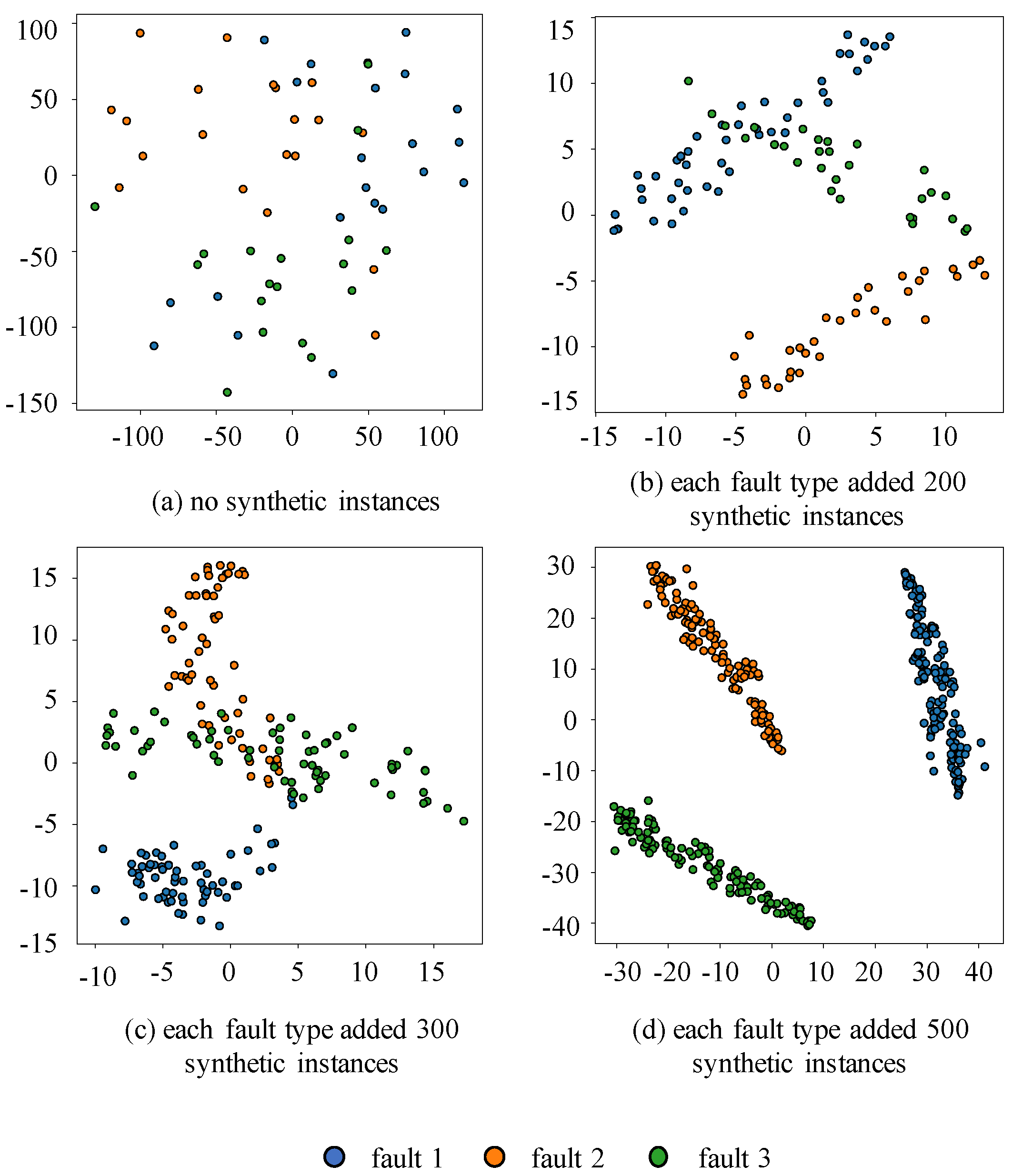
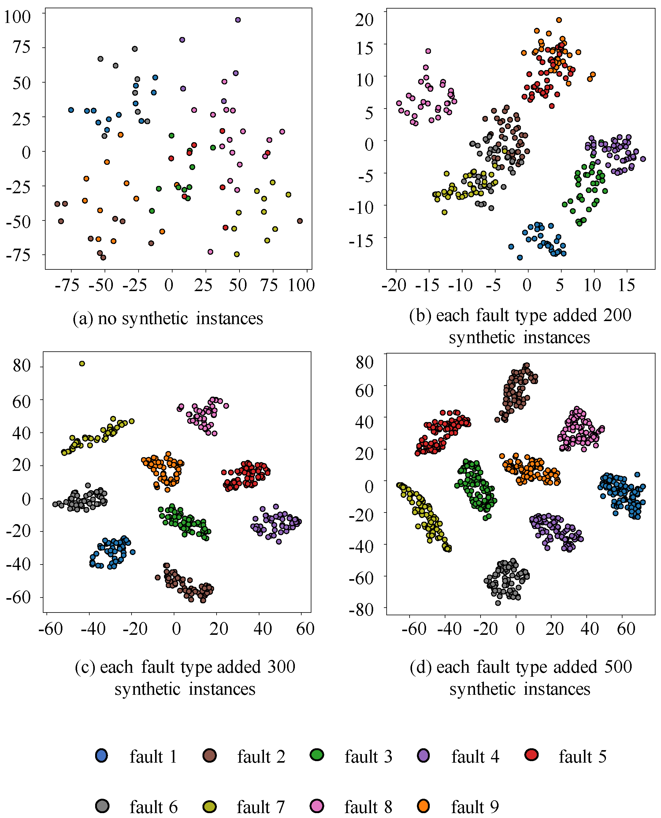
The experimental results for the three categories of faults dataset are shown in Figure 7. First, we selected 20 instances from each type of fault data randomly, and then used T-SNE to reduce the dimensionality of these data and visualize their distribution on a two-dimensional plane. As shown in Figure 7a, all three types of fault data were clustered together and could not be distinguished from each other due to a lack of sufficient data. This is why the data-driven classifier fails in the absence of sufficient data. Then, 200 synthetic fault instances generated by MFGAN were added to each type of fault data, and their distribution is shown in Figure 7b. It can be seen that the different types of fault data are significantly different, but the two types of fault data still overlap. We continued to increase the synthetic fault data until the number of synthetic data for each type of fault reached 500, as shown in Figure 7d. At this point, the three types of fault data have separated from each other while forming distinct clusters of clusters. The same occurred in Figure 8, which shows the results of visualizing the nine categories of faults dataset after T-SNE downscaling. The experiments show that through MFGAN, it is possible to capture different classes of valid features and synthesize high-quality data, bringing more discriminative information to the classification and making the synthesized fault data quite valid and realistic.

4.4.2. Performance and Generality of MFGAN

In industrial applications, it is difficult to collect fault data, which would pose a challenge for multiple types of fault diagnosis. We use multiple types of fault data and normal data to construct a complex unbalanced training dataset D_i. Then, the fault data and normal data are used to form a balanced test dataset D_t. Specifically, for the three categories of faults dataset, we set the initial ratio of D_i to 10:10:10:400. The number of normal data is 400 and the number of each type of fault data is 10. In the test dataset D_t, the number of each type of data is 100. For the nine categories of faults dataset, we set the initial ratio of D_i to 10:10:10:10:10:10:10:10:10:10:10:500. The number of normal data is 500 and the number of each type of fault data is 10. In the test dataset D_t, the number of each type of data is 100.

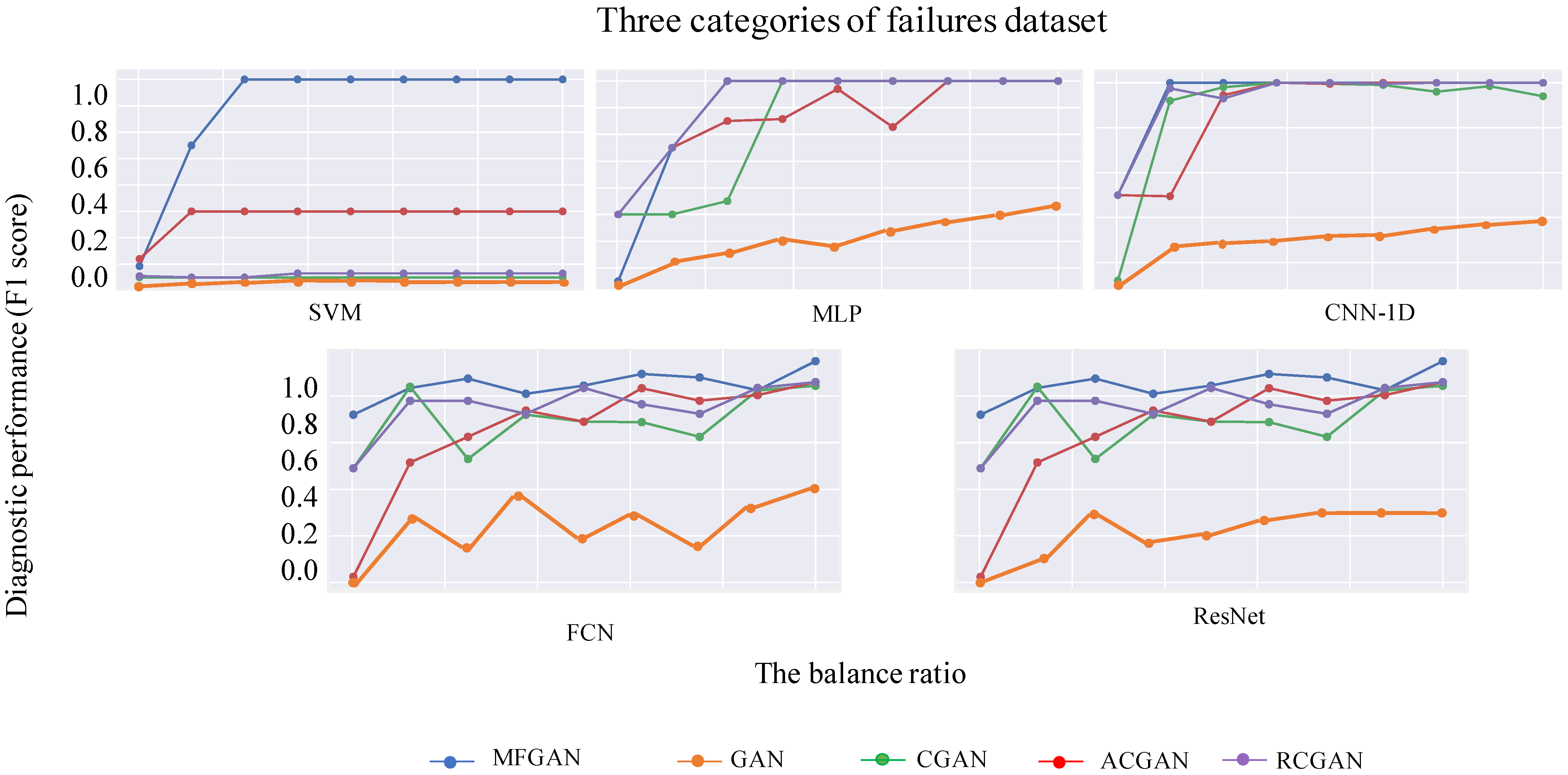
The numbers in the first row of

Table 4. Performance of MFGAN for different classifiers on the three categories of faults dataset.

Number of Augmented Instances	Fault Diagnosis Performance (F1 Score)
	SVM	MLP	CNN-1D	FCN	ResNet
0	0.293	0.500	0.750	0.860	0.878
50	0.710	0.750	1.000	0.918	0.918
100	1.000	1.000	0.990	0.938	0.978
150	1.000	1.000	1.000	0.905	0.980
200	1.000	1.000	1.000	0.923	0.988
250	1.000	1.000	1.000	0.948	0.980
300	1.000	1.000	1.000	0.940	0.983
350	1.000	1.000	1.000	0.913	0.985
400	1.000	1.000	1.000	0.975	0.975

indicate the number of synthetic instances added to D_i generated by MFGAN. The rest of the values represent the F1 scores of the different classifiers in D_t. It can be seen that the F1 scores of all classifiers increase with the number of synthetic fault instances added. This indicates that the fault data synthesized by MFGAN can bring more discriminative information to help the classifiers learn the correct separation boundaries. Figure 9 and Figure 10 represent the classification results of classifiers trained by fault data synthesized by different generation models on D_t. It can be seen that, for different D_i and different classifiers, the classifier trained by the fault data synthesized by MFGAN always has the best performance.

Table 5. Performance of MFGAN for different classifiers on the nine categories of faults dataset.

Number of Augmented Instances	Fault Diagnosis Performance (F1 Score)
	SVM	MLP	CNN-1D	FCN	ResNet
0	0.160	0.500	0.500	0.859	0.875
50	0.500	1.00	0.998	0.920	0.898
100	0.726	1.000	1.000	0.891	0.935
150	1.000	1.000	1.000	0.936	0.948
200	1.000	1.000	1.000	0.913	0.945
250	1.000	1.000	1.000	0.954	0.912
300	1.000	1.000	1.000	0.969	0.898
350	1.000	1.000	1.000	0.955	0.958
400	1.000	1.000	1.000	0.953	0.956
450	1.000	1.000	1.000	0.954	0.951
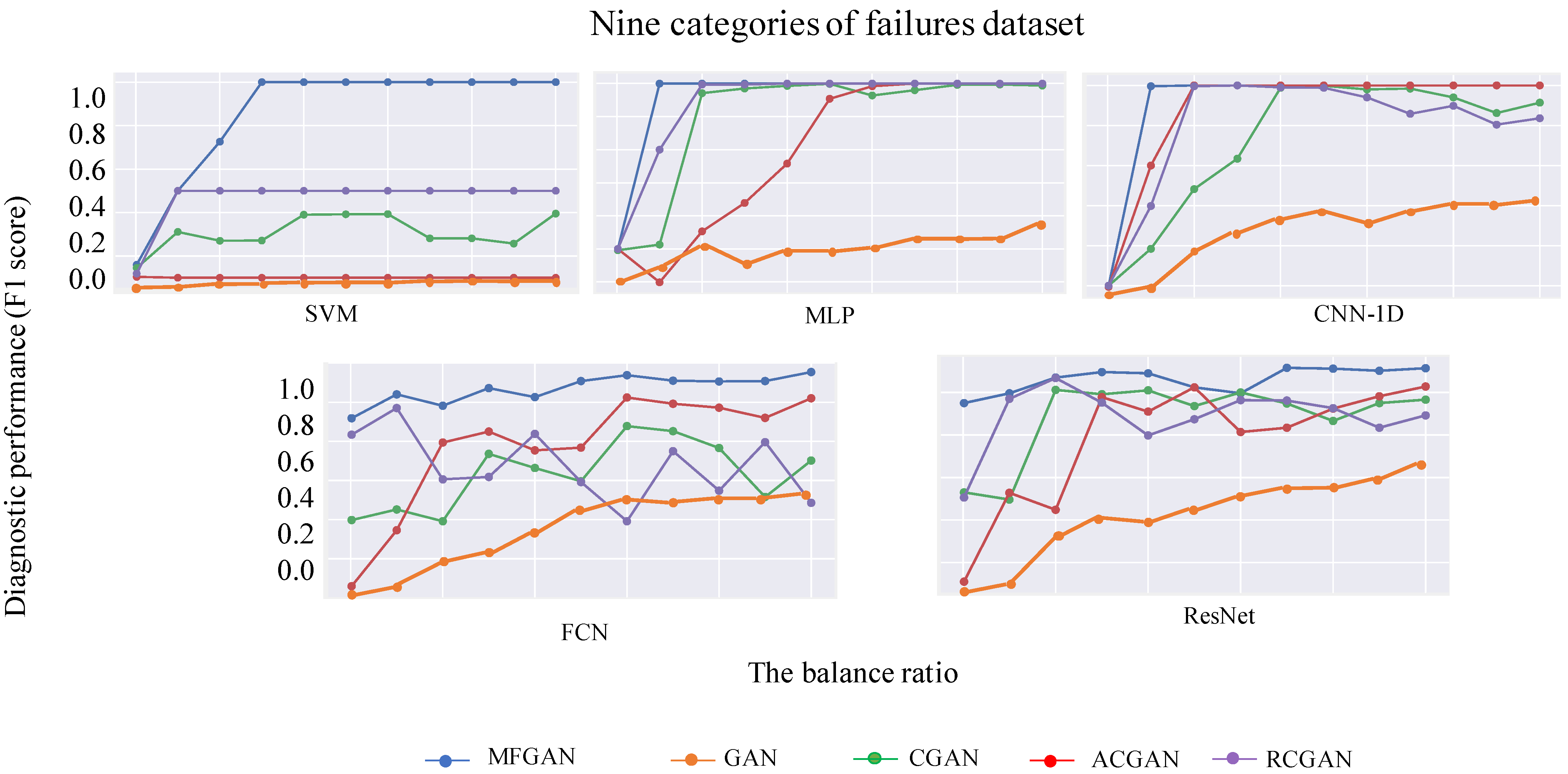
500	1.000	1.000	1.000	0.977	0.957

and Figure 10 show the experiment results on the nine categories of faults dataset, which are similar with that of the three categories of faults dataset. In Table 5, F1 scores of all classifiers are also increasing with the increase of synthetic fault instances added, and in Figure 9 and Figure 10, the fault data synthesized by MFGAN always have the best performance. To sum up, we can draw the following conclusions: (1) compared with other generative comparison models, MFGAN shows the best results on gradually balanced datasets among different classifiers, indicating that MFGAN synthesizes the highest quality fault instances, and proves that MFGAN has generality; (2) balanced datasets after being supplemented by good data can significantly improve the training effect and performance of classifiers.

4.4.3. Effectiveness of Feature Transfer Strategies

Table 6. Comparison of Euclidean distance in the three categories of faults dataset.

Category	Normal Data	Uniformly Distributed Noise	Standard Normal Distribution Noise
fault1	76.898	97.778	241.768
fault2	43.474	111.567	231.037
fault3	87.655	91.972	244.148

and

Table 7. Comparison of DTW distance in the three categories of faults dataset.

Category	Normal Data	Uniformly Distributed Noise	Standard Normal Distribution Noise
fault1	543.605	691.220	1709.199
fault2	307.282	788.811	1633.360
fault3	619.165	650.098	1725.932

represent the experimental results on the three categories of faults dataset. Table 6 uses Euclidean distance to evaluate the difference between the data, and Table 7 uses DTW (Dynamic Time Warping) distance. In the table, the first column represents the distance between fault data and normal data, the second column represents the distance between noise obeying uniformly distribution and normal data, and the third column represents the distance value between noise obeying standard normal distribution and normal data. It can be seen that the distance between all types of fault data and normal data is the minimum, which will reduce the difficulty of synthesizing fault data. This is also the reason why MFGAN can generate higher quality fault data. We obtained similar results on the nine categories of faults dataset, as shown in

Table 8. Comparison of Euclidean distance in the nine categories of faults dataset.

Category	Normal Data	Uniformly Distributed Noise	Standard Normal Distribution Noise
fault1	47.611	164.854	322.914
fault2	51.878	162.893	324.005
fault3	49.324	165.693	323.005
fault4	88.812	145.785	333.944
fault5	55.535	156.932	324.238
fault6	89.096	144.817	334.050
fault7	102.261	138.275	336.858
fault8	49.456	165.121	322.866
fault9	116.670	130.526	343.236

and

Table 9. Comparison of DTW in the nine categories of faults dataset.

Category	Normal Data	Uniformly Distributed Noise	Standard Normal Distribution Noise
fault1	475.846	1648.304	3228.351
fault2	516.868	1628.181	3239.231
fault3	492.986	1656.742	3229.276
fault4	887.850	1457.344	3338.659
fault5	554.594	1568.904	3241.597
fault6	890.105	1447.650	3339.695
fault7	1022.121	1382.086	3367.754
fault8	494.281	1651.009	3227.906
fault9	1165.438	1304.594	3431.442

. Meanwhile, the specific relationship between different specific faults and normal data is also analyzed. In Table 6 and Table 7, fault2, representing the inner ring fault, is always a smaller distance from the normal data, indicating that in the case of the three types of fault operation, the inner ring fault is to a lesser extent relative to the other faults, the ball to a lesser extent and the outer ring to the greatest extent of damage. In Table 8 and Table 9, fault1 to fault6, representing both ball faults and inner ring faults, are always at a smaller distance from the normal data, indicating that the outer ring is damaged to the greatest extent in the nine types of faulty operation.

To sum up, we verify that the distance between normal data and fault data is closer through experiments, and explain that the data-synthesis method based on feature transfer can obtain higher-quality data.

5. Conclusions

This article proposes a novel data augmentation method (MFGAN) for imbalanced fault diagnosis. MFGAN introduces feature transfer into GANs to reduce the difficulty of data augmentation and make full use of the normal data. The generator maps the normal data into the fault data space to accomplish fault data augmentation. Moreover, it can be embedded into any generation model of similar tasks, so it has good generality. Meanwhile, we extend the single discriminator to multi-scale ensemble discriminator architecture (MSED) to help MFGAN learn data features on multiple time scales to ensure more stable training and the high authenticity of the synthetic data. Finally, we apply the proposed data augmentation method to two rolling bearing datasets, and the experimental results show that the proposed method is superior. In practical applications, the amount of fault data may be too limited to support the training of MFGAN. Therefore, in future work, we will investigate more effective training of MFGAN under more data-poor conditions. Meanwhile, the data enhancement method proposed in this paper will also be extended to more scenarios with limited data.

References

- Zhang, X.; Chen, G.; Hao, T.; He, Z. Rolling Bearing Fault Convolutional Neural Network Diagnosis Method Based on Casing Signal. J. Mech. Sci. Technol. 2020, 34, 2307–2316. [Google Scholar] [CrossRef]
- Smith, W.A.; Randall, R.B. Rolling Element Bearing Diagnostics Using the Case Western Reserve University Data: A Benchmark Study. Mech. Syst. Signal Process. 2015, 64, 100–131. [Google Scholar] [CrossRef]
- Jiang, Q.; Yan, X. Multimode Process Monitoring Using Variational Bayesian Inference and Canonical Correlation Analysis. IEEE Trans. Autom. Sci. Eng. 2019, 16, 1814–1824. [Google Scholar] [CrossRef]
- Feng, J.; Wang, J.; Zhang, H.; Han, Z. Fault Diagnosis Method of Joint Fisher Discriminant Analysis Based on the Local and Global Manifold Learning and Its Kernel Version. IEEE Trans. Autom. Sci. Eng. 2016, 13, 122–133. [Google Scholar] [CrossRef]
- Chen, H.; Jiang, B. A Review of Fault Detection and Diagnosis for the Traction System in High-Speed Trains. IEEE Trans. Intell. Transp. Syst. 2020, 21, 450–465. [Google Scholar] [CrossRef]
- Huang, C.; Li, Y.; Loy, C.C.; Tang, X. Learning Deep Representation for Imbalanced Classification. In Proceedings of the IEEE Conference on Computer Vision and Pattern Recognition, Las Vegas, NV, USA, 27–30 June 2016; pp. 5375–5384. [Google Scholar]
- He, H.; Garcia, E.A. Learning from Imbalanced Data. IEEE Trans. Knowl. Data Eng. 2009, 21, 1263–1284. [Google Scholar]
- Zhao, Y.; Hao, K.; Tang, X.; Chen, L.; Wei, B. A Conditional Variational Autoencoder Based Self-Transferred Algorithm for Imbalanced Classification. Knowl.-Based Syst. 2021, 218, 106756. [Google Scholar] [CrossRef]
- Chen, B.; Xia, S.; Chen, Z.; Wang, B.; Wang, G. RSMOTE: A Self-Adaptive Robust SMOTE for Imbalanced Problems with Label Noise. Inf. Sci. 2021, 553, 397–428. [Google Scholar] [CrossRef]
- Gu, X.; Angelov, P.P.; Soares, E.A. A Self-Adaptive Synthetic over-Sampling Technique for Imbalanced Classification. Int. J. Intell. Syst. 2020, 35, 923–943. [Google Scholar] [CrossRef]
- Drummond, C.; Holte, R.C. C4. 5, Class Imbalance, and Cost Sensitivity: Why Under-Sampling Beats Over-Sampling. In Proceedings of the Workshop on Learning from Imbalanced Datasets II, Washington, DC, USA, 21 August 2003; Volume 11, pp. 1–8. [Google Scholar]
- Feng, F.; Li, K.-C.; Shen, J.; Zhou, Q.; Yang, X. Using Cost-Sensitive Learning and Feature Selection Algorithms to Improve the Performance of Imbalanced Classification. IEEE Access 2020, 8, 69979–69996. [Google Scholar] [CrossRef]
- Haixiang, G.; Yijing, L.; Shang, J.; Mingyun, G.; Yuanyue, H.; Bing, G. Learning from Class-Imbalanced Data: Review of Methods and Applications. Expert Syst. Appl. 2017, 73, 220–239. [Google Scholar] [CrossRef]
- Goodfellow, I.; Pouget-Abadie, J.; Mirza, M.; Xu, B.; Warde-Farley, D.; Ozair, S.; Courville, A.; Bengio, Y. Generative Adversarial Nets. Adv. Neural Inf. Process. Syst. 2014, 27, 2672–2680. [Google Scholar]
- Kazeminia, S.; Baur, C.; Kuijper, A.; van Ginneken, B.; Navab, N.; Albarqouni, S.; Mukhopadhyay, A. GANs for Medical Image Analysis. Artif. Intell. Med. 2020, 109, 101938. [Google Scholar] [CrossRef]
- Donahue, C.; McAuley, J.; Puckette, M. Synthesizing Audio with GANs. 2018. Available online: https://openreview.net/forum?id=r1RwYIJPM (accessed on 6 April 2022).
- Fu, Z.; Xian, Y.; Geng, S.; Ge, Y.; Wang, Y.; Dong, X.; Wang, G.; De Melo, G. ABSent: Cross-Lingual Sentence Representation Mapping with Bidirectional GANs. In Proceedings of the AAAI Conference on Artificial Intelligence, New York, NY, USA, 7–12 February 2020; Volume 34, pp. 7756–7763. [Google Scholar]
- Guo, L.; Lei, Y.; Xing, S.; Yan, T.; Li, N. Deep Convolutional Transfer Learning Network: A New Method for Intelligent Fault Diagnosis of Machines with Unlabeled Data. IEEE Trans. Ind. Electron. 2018, 66, 7316–7325. [Google Scholar] [CrossRef]
- Gulrajani, I.; Ahmed, F.; Arjovsky, M.; Dumoulin, V.; Courville, A.C. Improved Training of Wasserstein Gans. Adv. Neural Inf. Process. Syst. 2017, 30, 5769–5779. [Google Scholar]
- Le, H.L.; Landa-Silva, D.; Galar, M.; Garcia, S.; Triguero, I. EUSC: A Clustering-Based Surrogate Model to Accelerate Evolutionary Undersampling in Imbalanced Classification. Appl. Soft Comput. 2021, 101, 107033. [Google Scholar] [CrossRef]
- Liu, T.; Zhu, X.; Pedrycz, W.; Li, Z. A Design of Information Granule-Based under-Sampling Method in Imbalanced Data Classification. Soft Comput. 2020, 24, 17333–17347. [Google Scholar] [CrossRef]
- Chawla, N.V.; Bowyer, K.W.; Hall, L.O.; Kegelmeyer, W.P. SMOTE: Synthetic Minority over-Sampling Technique. J. Artif. Intell. Res. 2002, 16, 321–357. [Google Scholar] [CrossRef]
- Hu, S.; Liang, Y.; Ma, L.; He, Y. MSMOTE: Improving Classification Performance When Training Data Is Imbalanced. In Proceedings of the 2009 Second International Workshop on Computer Science and Engineering, Qingdao, China, 28–30 October 2009; Volume 2, pp. 13–17. [Google Scholar]
- Han, H.; Wang, W.-Y.; Mao, B.-H. Borderline-SMOTE: A New over-Sampling Method in Imbalanced Data Sets Learning. In International Conference on Intelligent Computing; Springer: Berlin/Heidelberg, Germany, 2005; pp. 878–887. [Google Scholar]
- Sun, J.; Shang, Z.; Li, H. Imbalance-Oriented SVM Methods for Financial Distress Prediction: A Comparative Study among the New SB-SVM-Ensemble Method and Traditional Methods. J. Oper. Res. Soc. 2014, 65, 1905–1919. [Google Scholar] [CrossRef]
- Raghuwanshi, B.S.; Shukla, S. SMOTE Based Class-Specific Extreme Learning Machine for Imbalanced Learning. Knowl.-Based Syst. 2020, 187, 104814. [Google Scholar] [CrossRef]
- Galar, M.; Fernandez, A.; Barrenechea, E.; Bustince, H.; Herrera, F. A Review on Ensembles for the Class Imbalance Problem: Bagging-, Boosting-, and Hybrid-Based Approaches. IEEE Trans. Syst. Man Cybern. Part C (Appl. Rev.) 2011, 42, 463–484. [Google Scholar] [CrossRef]
- Maldonado, S.; Weber, R.; Famili, F. Feature Selection for High-Dimensional Class-Imbalanced Data Sets Using Support Vector Machines. Inf. Sci. 2014, 286, 228–246. [Google Scholar] [CrossRef]
- Cheng, F.; Zhang, J.; Wen, C. Cost-Sensitive Large Margin Distribution Machine for Classification of Imbalanced Data. Pattern Recognit. Lett. 2016, 80, 107–112. [Google Scholar] [CrossRef]
- Ghazikhani, A.; Monsefi, R.; Sadoghi Yazdi, H. Online Cost-Sensitive Neural Network Classifiers for Non-Stationary and Imbalanced Data Streams. Neural Comput. Appl. 2013, 23, 1283–1295. [Google Scholar] [CrossRef]
- Datta, S.; Das, S. Near-Bayesian Support Vector Machines for Imbalanced Data Classification with Equal or Unequal Misclassification Costs. Neural Netw. 2015, 70, 39–52. [Google Scholar] [CrossRef] [PubMed]
- Mirza, M.; Osindero, S. Conditional Generative Adversarial Nets. arXiv 2014, arXiv:1411.1784. [Google Scholar]
- Odena, A.; Olah, C.; Shlens, J. Conditional Image Synthesis with Auxiliary Classifier Gans. In Proceedings of the International Conference on Machine Learning, Sydney, Australia, 6–11 August 2017; pp. 2642–2651. [Google Scholar]
- Zheng, T.; Song, L.; Wang, J.; Teng, W.; Xu, X.; Ma, C. Data Synthesis Using Dual Discriminator Conditional Generative Adversarial Networks for Imbalanced Fault Diagnosis of Rolling Bearings. Measurement 2020, 158, 107741. [Google Scholar] [CrossRef]
- Xu, D.; Yuan, S.; Zhang, L.; Wu, X. Fairgan+: Achieving Fair Data Generation and Classification through Generative Adversarial Nets. In Proceedings of the 2019 IEEE International Conference on Big Data (Big Data), Los Angeles, CA, USA, 9–12 December 2019; pp. 1401–1406. [Google Scholar]
- Erol, B.; Gurbuz, S.Z.; Amin, M.G. Motion Classification Using Kinematically Sifted ACGAN-Synthesized Radar Micro-Doppler Signatures. IEEE Trans. Aerosp. Electron. Syst. 2020, 56, 3197–3213. [Google Scholar] [CrossRef] [Green Version]
- Yu, L.; Zhang, W.; Wang, J.; Yu, Y. Seqgan: Sequence Generative Adversarial Nets with Policy Gradient. In Proceedings of the Proceedings of the AAAI Conference on Artificial Intelligence, San Francisco, CA, USA, 4–9 February 2017; Volume 31. [Google Scholar]
- Lee, S.; Hwang, U.; Min, S.; Yoon, S. Polyphonic Music Generation with Sequence Generative Adversarial Networks. arXiv 2017, arXiv:1710.11418. [Google Scholar]
- Esteban, C.; Hyland, S.L.; Rätsch, G. Real-Valued (Medical) Time Series Generation with Recurrent Conditional Gans. arXiv 2017, arXiv:1706.02633. [Google Scholar]
- Mao, Q.; Lee, H.-Y.; Tseng, H.-Y.; Ma, S.; Yang, M.-H. Mode Seeking Generative Adversarial Networks for Diverse Image Synthesis. In Proceedings of the IEEE/CVF Conference on Computer Vision and Pattern Recognition, Long Beach, CA, USA, 15–20 June 2019; pp. 1429–1437. [Google Scholar]
- Wang, Z.; Yan, W.; Oates, T. Time Series Classification from Scratch with Deep Neural Networks: A Strong Baseline. arXiv 2016, arXiv:1611.06455. [Google Scholar] [CrossRef]
Figure 1.
Highly-skewed class distribution data causes the classifier to work poorly.
Figure 2.
Overall framework comparisons of vanilla GAN, CGAN, ACGAN and RCGAN.
Figure 3.
Overall framework of MFGAN.
Figure 4.
The structure of Generator in MFGAN.
Figure 5.
The structure of Discriminator in MFGAN.
Figure 6.
Figure 7.
T-SNE Visualization of Different Quantities of Synthetic Data (Three Categories of Faults).
Figure 8.
T-SNE Visualization of Different Quantities of Synthetic Data (Nine Categories of Faults).
Figure 9.
Comparison of F1 score across different imbalanced percentages in three categories of faults dataset.
Figure 10.
Comparison of F1 score across different imbalanced percentages in nine categories of faults dataset.