
Multibody Model for the Design of a Rover for Agricultural Applications: A Preliminary Study


Department of Industrial Engineering, University of Naples “Federico II”, Via Claudio 21, 80125 Napoli, Italy
*
Authors to whom correspondence should be addressed.
Machines 2022, 10(4), 235; https://doi.org/10.3390/machines10040235
Submission received: 14 February 2022
/
Revised: 15 March 2022
/
Accepted: 25 March 2022
/
Published: 27 March 2022
(This article belongs to the Special Issue Dynamic Analysis of Multibody Mechanical Systems)
Abstract
:The employment of vehicles such as rovers equipped with automictic and robotic systems in agriculture is an emerging field. The development of suitable simulation models can aid in the design and testing of agricultural rovers before prototyping. Here, we propose a simulation test rig based on a multibody model to investigate the main issues connected with agricultural rover designs. The results of the simulations show significant differences between the two structures, especially regarding the energy savings, which is a key aspect for the applicability of a rover in field operations. The modular structure of the proposed simulation model can be easily adapted to other vehicle structures.
1. Introduction
In the last ten years, increasing interest has emerged in the development of robotic and automation systems for field operations [1,2,3]. In this context, research groups, both in academia and industry, have paid attention to the application of robotics in the agricultural field [4,5]. Robotics for agricultural purposes can aid the execution of repetitive and heavy manual operations improving, the conditions of agricultural workers [6]. Fruit harvesting offers significant opportunities for the field of agricultural robotics, and has, thus, gained much attention in recent decades. Indeed, several robots have been developed for harvesting fruits and vegetables [7,8,9].
Robotic systems can enhance precision agricultural tasks, for example in the harvesting process in which robots equipped with vision perception sensors can understand when and which fruit must be picked at a given time according to the maturation phase [10,11,12,13]. To face these tasks, proper algorithms [14,15,16,17] must be integrated into the hardware systems to process data acquired from the surroundings, as well as to control the end effector trajectory, for instance through low-cost RGB-D cameras [18,19].
Furthermore, both the academic community and the industry are showing a radical growth of interest in agricultural robotics, and in particular in unmanned service robotics and vehicles [20,21,22,23,24,25,26]. Some autonomous vehicles designed for agricultural tasks have been already been presented in recent years [27,28,29]. Agricultural rovers, similarly to rovers employed to explore planets in orbits, such as Curiosity and Perseverance Mars rovers, are autonomous or remotely controlled vehicles able to tread on terrain and perform various operations. Agri_q [30,31] is an agricultural rover designed by Politecnico di Torino (Turin, Italy) with the aim of performing crop monitoring and to permit landing, carrying and recharging tasks by aerial robots.
In this context, the development of a suitable simulation environment can aid in the design and testing of these vehicles in complex scenarios [32,33,34,35]. The main issue in agricultural rover design is the ability of these robots to operate in unstructured agricultural environments. Moreover, such vehicles must rapidly adapt to the variability of the environment, and for this reason must be equipped with perception sensors. The agricultural rovers should be able to perform tasks, meaning they require a proper end effector design [36]. They must ensure human safety and the preservation of the environment. Multibody simulation models offer the possibility of carrying out multiple performance analyses of mechanical systems, and in particular for vehicles that can be tested in both static and dynamic conditions in multiple environments [37,38,39,40,41,42].
In this paper, we address some of the challenges of working in unstructured farming environments through the development of a simulation test rig based on a multibody simulation environment. The model accounts for contact analysis between the vehicle and ground. In this way, it is possible to study the performance of an agricultural rover from multiple angles. This agricultural rover should be able to perform several tasks while moving in agricultural areas such as vineyards. Indeed, in a future design effort, the rover will be equipped with an articulated robotic arm mounted with different end effectors.
Simulation results drive the rover design process step by step. Indeed, the simulation test rig allows us to analyze the rollover effects in static conditions, the motor sizing, the rover dynamics in rough environments, the rover suspension system, and the energy consumption. Two main vehicle structures are tested, which differ only in their suspension systems—one equipped with a linear damped system, while the other equipped with a rocker-bogie system, similarly to the space exploration rovers [43,44]. The main contributions of this paper are as follows. Section 2 provides a description of the simulation test rig with a multibody model, the equations adopted in the contact model, and the two rover structures used for the two case studies in this paper. Section 3 presents a brief description of the simulation conditions and discusses the results for the different aspects analyzed in the rover design phases. In the remaining section of the manuscript, the suspension performance and energy consumption are examined using multibody simulations on uneven terrain. Certain aspects are also discussed in relation to the control system adopted by the vehicle. As a final remark, an overview of the energy saving results is depicted for the two rover structures moving at two different velocities. This aspect makes the developed test rig particularly useful, allowing an indicative estimation of the consumption of these vehicles before designing them.
2. Materials and Methods
2.1. Multibody Model Description
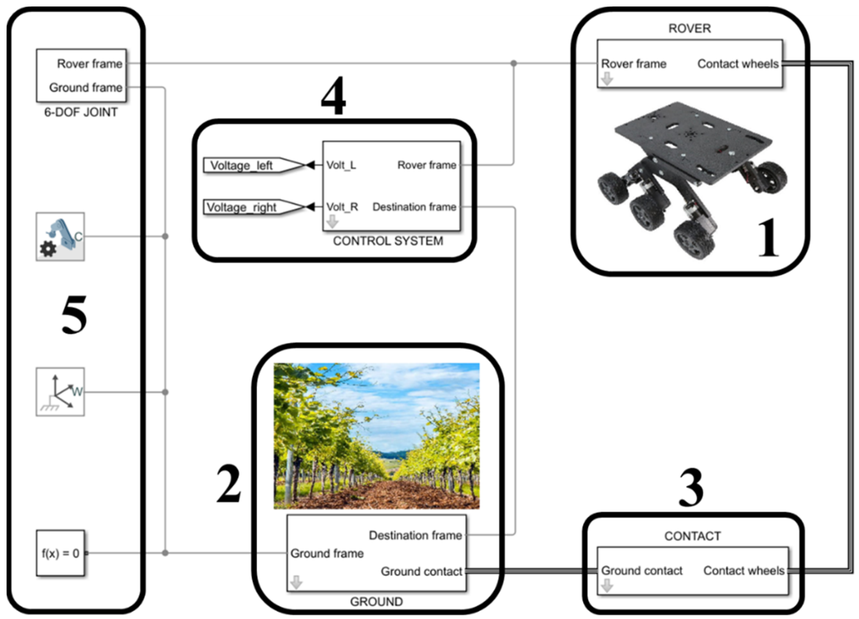
The multibody model reported in Figure 1 was developed in the MATLAB environment (©Mathworks, Natick, MA, USA) by employing the Simscape™ Library, which enables the rapid creation of physical component models based on physical connections that directly integrate with block diagrams and other modeling paradigms. The model can be divided in five main blocks, as shown in Figure 1.
The first block accounts for the rover structural part and its power electronic system.
The multibody rover structure is designed by employing a sequence of rgid bodies, flexible bodies, and joints. Some joints are connected to motors that drive the motion of the rover parts and actuation system. In this way, in the model there is a connection between the rotational mechanics and electrical domain. In the second block, there is a multibody model of the ground. The ground is composed of several rigid bodies. The combination of the bodies allows different ground conditions and ground inclinations to be modeled and for proper obstacles to bed added to the rover’s path. The third block models the wheel–ground interaction through a contact model. Briefly, the contact block models the contact between a pair of bodies using the penalty method. This method allows the bodies to penetrate by a small amount to compute the contact forces. The block applies normal and frictional contact forces between the connected base and follower bodies. The normal contact force is computed using the force equation of the classical spring–damper system. During contact, the normal contact force is proportional to its corresponding penetration depth and velocity. The transition region width specifies the transitional region in the force equations. While the penetration depth moves through the transition region, the block smoothly ramps up the force. At the end of the transition region, full stiffness and damping are applied. On the rebound, both the stiffness and damping forces are smoothly decreased back to zero.
The normal force (fn) and friction force (ff) can be written as in the following Equations (1) and (2):
where σ is the damping coefficient, k is the spring stiffness, z is the depth penetration, ż is the penetration velocity, (Vr) is the relative tangential velocity, and μ(Vr) is the friction coefficient that depends on (Vr).
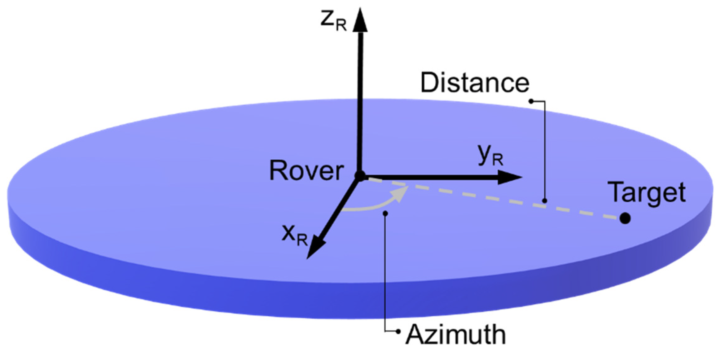
The fourth block models the control system. This block sets the tension to be applied to the motors to reach a desired destination. The control unit computes data while accounting for motor specifications and the desired performance. Moreover, it identifies the relative position between the desired destination and the current rover position due to two main parameters. The first parameter is the orientation angle between the rover’s direction of travel and the segment joining the rover’s center and the desired destination object. The second parameter is the distance between the rover and the desired object.
The fifth block defines the global reference system used to identify the relative position of the rover with respect to the ground and the gravity force action.
2.2. Rover Structure Description
The previously described multibody model allows multiphysics simulations of vehicles with different main geometric parameters. Indeed, block 1 of the model defines the structure and the actuation of the system, which can be easily substituted to be adapted to other rover structures.
The general rover structure was defined using proper simulations. In particular, the rover’s encumbrance must be the minimum value to be used in different environments and to decrease the overall energy consumption. The rover must possess high agility to overcome possible obstacles in the path. Moreover, the rover’s center of mass must be designed to achieve a good compromise between stability and agility. To ensure the applicability of the rover in unstructured agricultural environments, certain design specifications that must be met were identified. For the this rover to work in grape vineyards, certain design specifications have been stated, as follows: a maximum ground inclination range of 30–40 degrees, maximum overall lateral size of 1 m, vehicle velocity of around 5 km/h, maximum size of obstacles to be avoided of 0.2 m, and electric autonomy lasting at least 40 min. The wheels use skid steering mode to let the vehicle change its orientation.
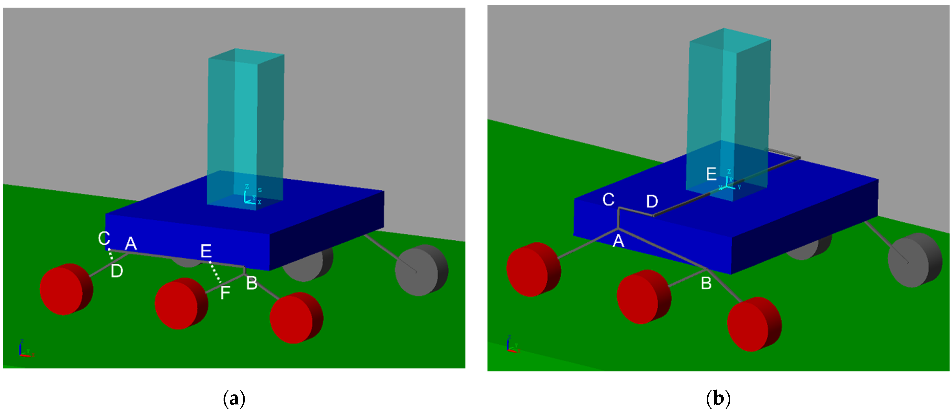
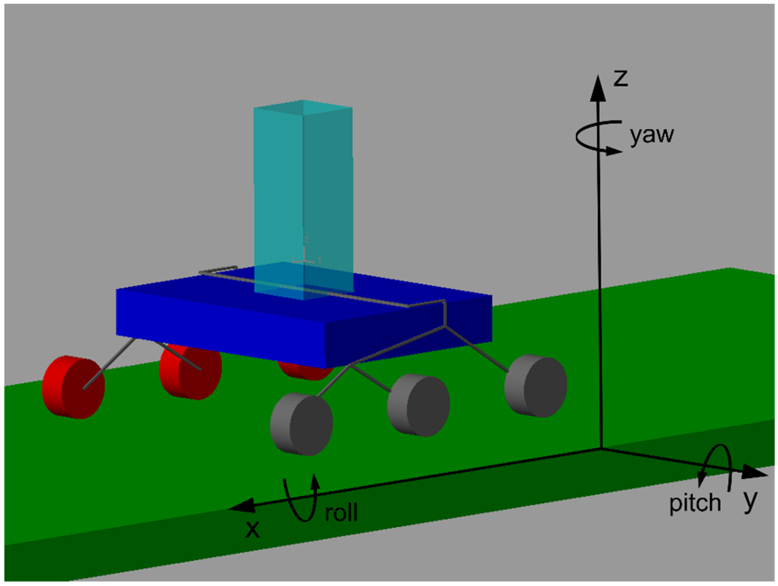
For the purposes of this paper, two main rover structures, as shown in Figure 2, were identified and simulated. The two rovers have six wheels actuated with six electric motors.
The wheels were modeled using cylindrical elements measuring 0.13 m in diameter and 0.06 m in height. The main difference between the two structures is the suspension system. For clarity, the first structure will be named the linear suspension rover (LSR), while the second structure will be named the rocker-bogie rover (RBR).
The linear suspension rover shown in Figure 2a uses two independent linear spring–damper suspension systems, one on the rear part () and one on the front part (); A and B points represent rotational joints with the rotational axis parallel to the wheels’ rotation axis. The rocker-bogie rover (Figure 2b) uses the suspension system employed by the rovers used for space exploration [43,44]. In Figure 2b, points A, B, and C represent rotational joints with the rotational axis parallel to the wheels’ rotation axis, while points D and E are rotational joints with axes perpendicular to the central slab. The flexible link is modeled using Euler–Bernoulli beam theory. Finally, joints B and E are linear spring–damper and damper elements, respectively.
The two rovers have the same total mass of 27 kg and a global vehicle envelope of 0.83 × 0.72 × 0.28 m. The weight accounts for the presence of six DC motors (0.5 kg each), one mounted on each wheel. Most of the structure weight is due to the presence of a robotic arm that was modeled as a solid prismatic element of 20 kg weight and with dimensions of 0.15 × 0.15 × 0.5 m.
2.3. Control Strategy
The control strategy was based on the idea that in a future design, the rover will be equipped with a camera able to acquire and process data from the surroundings. Using a vision system (for instance an RGB-D camera), the rover will identify the target to be achieved or the obstacles to be avoided. Proper algorithms will give the rover control system two main inputs, namely the distance and the azimuth angle, as depicted in Figure 3.
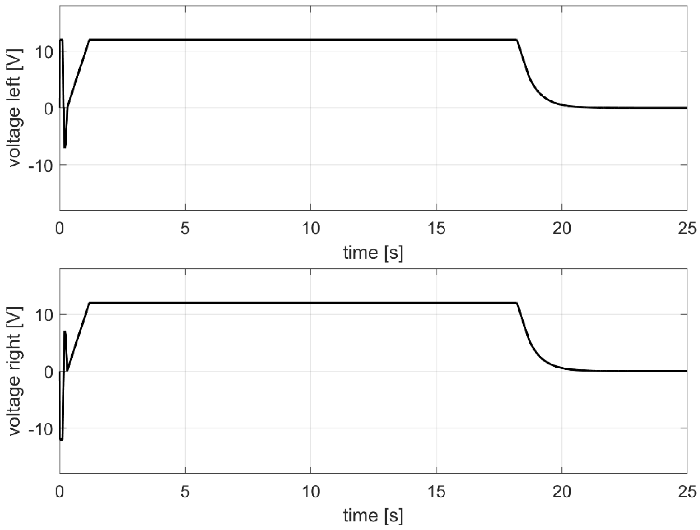
These values are the inputs for a proportional control strategy that enables the vehicle to change its initial orientation (azimuth) via the skid steering configuration and reach the desired position. To tune the control strategy for more precise vehicle performance, the saturation voltage was set to limit the acceleration of the right and left wheel sides independently. The saturation limits had higher values during the orientation phase with respect to the vehicles’ forward motion. Indeed, during the first control stage, our aim was to let the vehicle quickly change its direction. When the vehicle moves in the forward direction, the saturation voltage allows for velocity control of the vehicle in relation to the distance of the object to be reached. The input voltages for the wheel control unit for the left and right vehicle sides are in Figure 4.
2.4. Simulation Details
Table 1 summarizes the main parameters of the simulation campaign. Multibody simulation output results, which will be shown in the next paragraphs, aided in the rover design from multiple perspectives.
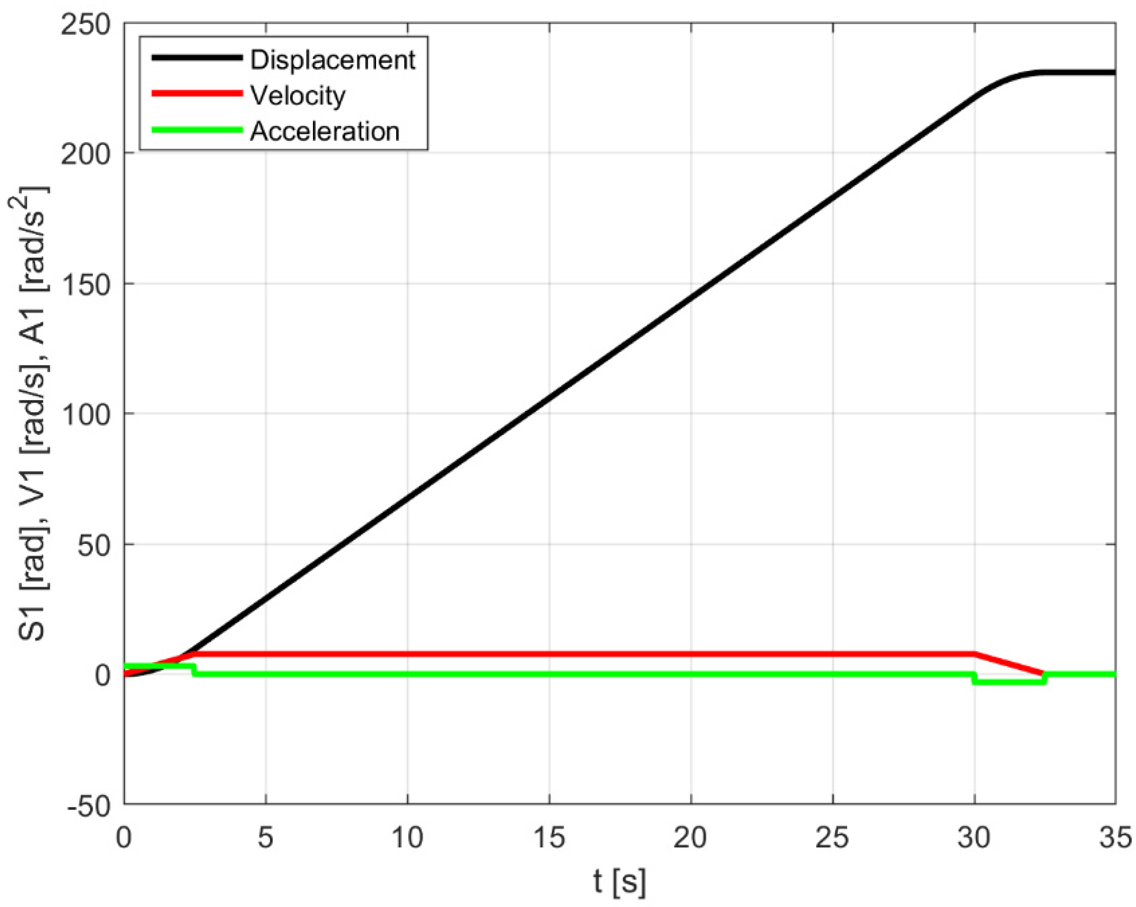
For inverse dynamics simulations, displacement, velocity, and acceleration profiles, as shown in Figure 5, are given as inputs to the rotational joint connected to each wheel.
3. Results and Discussion
The aim of this study was to show how the development of multibody models can aid in the design of a rover for agricultural applications. Simulations were carried out to investigate the different aspects of the design. Two rovers, differing only in their suspension systems, were considered as input vehicle structures. In this current study, the simulation results are presented in an attempt to detail the responses of each vehicle with changing simulation conditions and soil terrains. However, the simulation test rig can be easily adapted to other vehicles thanks to its modular design.
3.1. Rollover Study in Static Conditions
As a first study, the rollover stability of the rover structure was assessed. The simulation consisted of placing the rover on a sloped plane and changing the roll and pitch angles, as depicted in Figure 6. During the simulations, the rotation velocity of the six wheels was set to zero. Both the roll and the pitch angles were increased in one degree steps. The yaw angle was not considered as a design issue so far, given the possible future applicability of this rover for agricultural purposes.
The rollover study results are reported in Table 2 in terms of the maximum pitch and roll angles that were admissible before overturning for the two rover vehicles studied in this paper. The pitch and roll angles are independent values. Once the LSR overcomes a 45 degree roll angle, the vehicle overturns as long as the pitch angle is lower than the maximum admissible pitch of 41 degrees. At the same time, the RBR overturns when the ground inclination exceeds 45 degrees for the pitch and 37 degrees for the roll angle. Both rovers’ design specifications include the previously stated maximum ground inclination range of 30–40 degrees.
The pitch and roll angles for both structures will be important features when the specific rover workspace is established. The agricultural tasks will be related to the specific end effector mounted on the articulated robotic arm. When the rover has to work with its robotic arm fully extended to its right or left, it is clear that the maximum roll angle allowed is a fundamental design factor. The maximum pitch value will also be an important design factor when the rover works with the robotic arm fully extended to the rear or front. The maximum pitch and roll values take on great importance in terms of safety performance when humans and robotic vehicles have to share the same workspace.
3.2. Motor Sizing
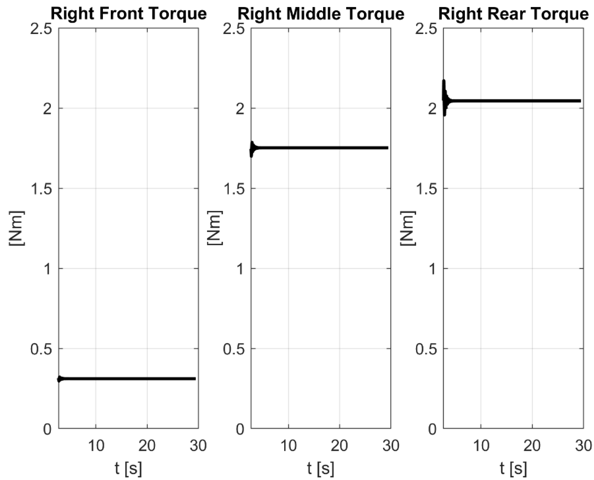
To assess the motor sizing of the rover, simulations were carried out on smooth soil using the inverse dynamics. These simulations incorporated the s-shaped motion law (displacement, velocity, and acceleration, shown in previous Figure 5) set as an input for the rover and the return torque values were computed for each wheel. In these simulations, the rover operated in critical conditions—the vehicle was placed on a sloped plane at 35 degrees with an acceleration of 0.2 m/s2 and velocity of 1.8 km/h. Figure 7 shows the results for the three right wheels: the maximum torque at equilibrium was 2.1 Nm, which was recorded on the rear wheel, and as expected these values decreased for the middle and front wheels. These values do not account for the initial transient values. The torque values presented in Figure 7 correspond to the period in which the velocity profile, as previously showed in Figure 5, was constant. The results were symmetrical and equal for the left side, and for this reason they are not reported.
Simulations were carried out for both structures adopted in this study, returning similar values as for the wheel torque values. The motor choice was the same for both structures, since they had the same global envelope dimensions and the same weight. The maximum value torque values allow one to choose a proper motor that will be used in subsequent simulations. Given the system velocity and maximum torque, it is possible to compute the motor power. Thus, in the rest of the study, the simulations were based on direct dynamics and the motor parameters were explicitly set. The motor parameters, given in Table 3, were set considering a DC commercial motor. Multiple simulation tests were run for a rover structure equipped with six DC motors, one for each wheel.
3.3. Rover Dynamics on Rough Soils
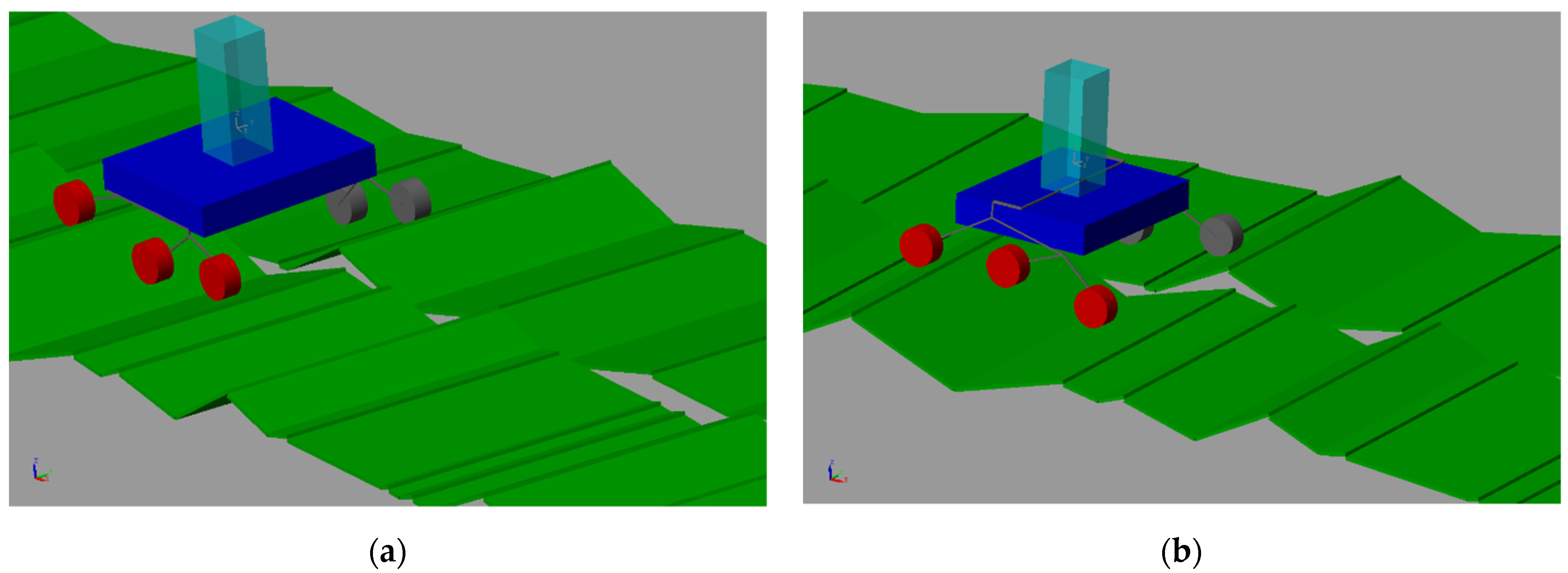
Direct dynamics simulations were carried out to study the rover dynamics in the unstructured environments in which the vehicle has to operate. The plane was modeled using a combination of solid brick elements. The path was composed of bricks of a random inclination and length. The ground in contact with the right wheels was different from that with the left wheels to increase the roughness of the ground and to make the simulation more similar to reality. This type of modeling seems appropriate to simulate the behavior of such vehicles in agricultural fields. Figure 8 shows two simulation frames for the LSR and the RBR on rough soil.
For the two type of vehicles, the simulations on rough soil allowed us to gain useful information on the rovers’ performance. To this end, the rover suspension sizing and energy consumption will be briefly described in the next sections.
3.3.1. Rover Suspension Performance
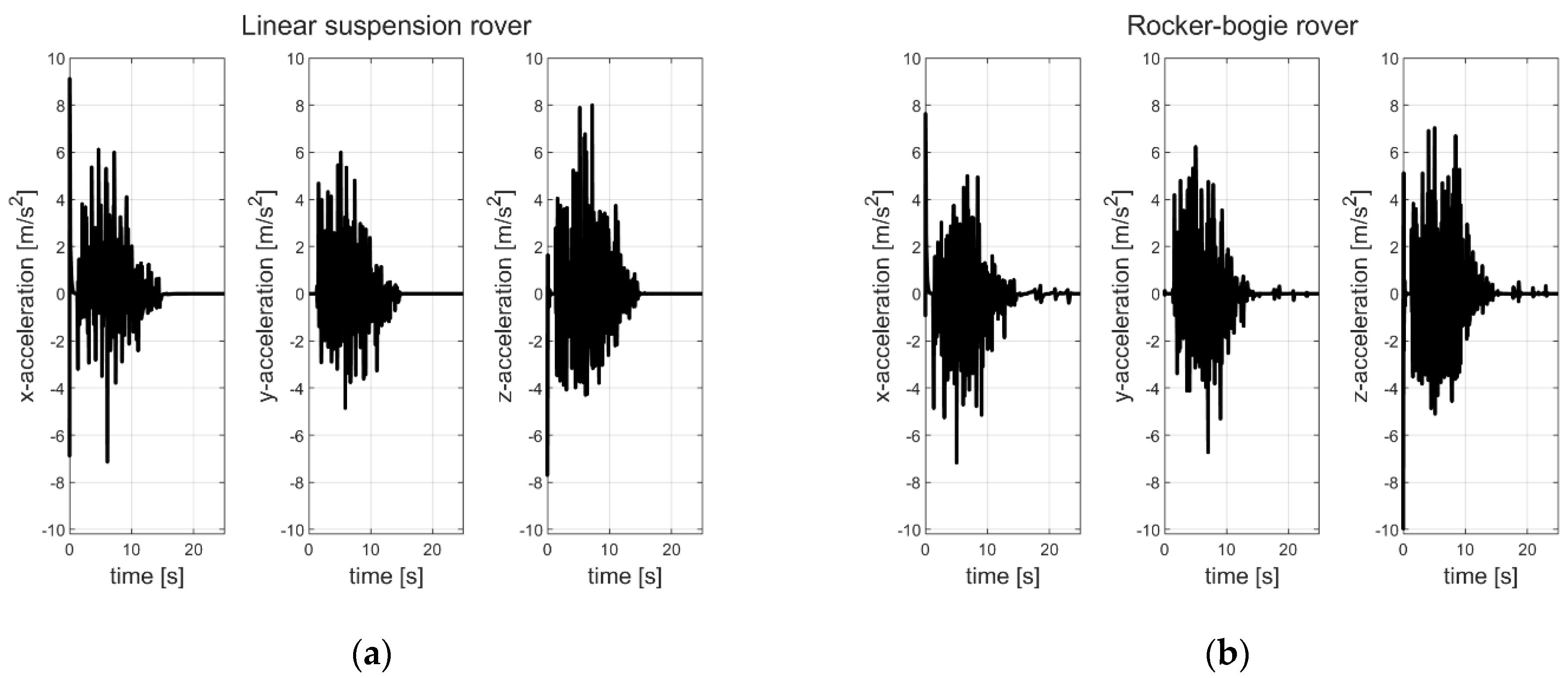
Preliminary simulations were carried out to set the proper stiffness and damping parameters. A first analysis allowed us to compare the vibration levels of the two structures. Figure 9 shows the acceleration signals computed on the chassis center for the two rovers along the three orthogonal directions x, y, and z, which are the axes of the global reference system. During the simulations on rough soil, the acceleration values were of the same order of magnitude in all three directions.
The RBR showed average acceleration values similar to those of the LSR for all three directions. The maximum absolute values for the LSR were 7.13, 5.99, and 7.99 m/s2 vs. 7.16, 6.73, and 7.03 m/s2 for the RBR (initial transient values were skipped in the calculation).
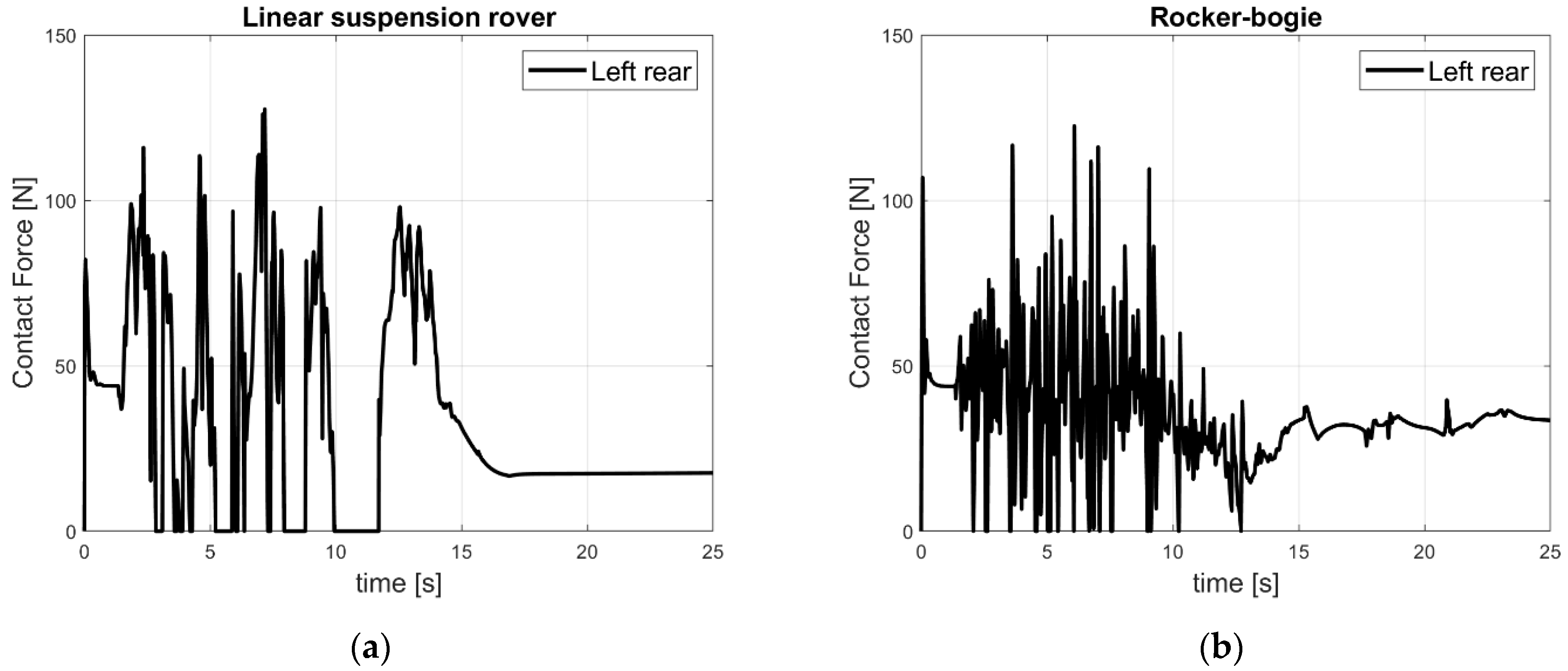
The simulation output allowed us to obtain an overall idea of the suspension performance for both structures. In Supplementary Materials Videos S1 and S2, these results are reported. One can be notice the better performance of the RBR with respect to the LSR. In Video S1, the rear left wheel seems to lift itself up from the ground for the linear suspension rover several times. A more detailed analysis of the contact force quantification between the wheels and the ground is shown in Figure 10. A contact force analysis was computed for the six wheels. Here, we report only the results for the left rear wheel for both vehicles. The whole analysis is reported in the Supplementary Materials for the six wheels of both rover structures (Figures S3 and S4). The high magnitude peaks for both the simulations results may have been caused by numerical integration issues during the motion equation integration.
For both vehicles, we computed the time at which the recorded contact force reached a zero value, as reported in Table 4. This value seems to be a representative parameter of the suspension performance. Indeed, when the contact force is equal to zero, there is no contact between the wheel and ground. The agricultural rovers should be able to overcome obstacles while keeping the wheels in contact with the ground. Over a simulation duration of 25 s, for the rocker-bogie rover this phenomenon occurred for a shorter time, highlighting the better performance of this vehicle in dealing with rough terrain. As reported in Table 4, all six wheels of the rocker-bogie rover maintained contact with the ground for almost the whole duration of the simulation. Each wheel lost contact with ground for less than 1 s over the 25 s simulation time.
3.3.2. Electric Motor Absorbed Power Estimation
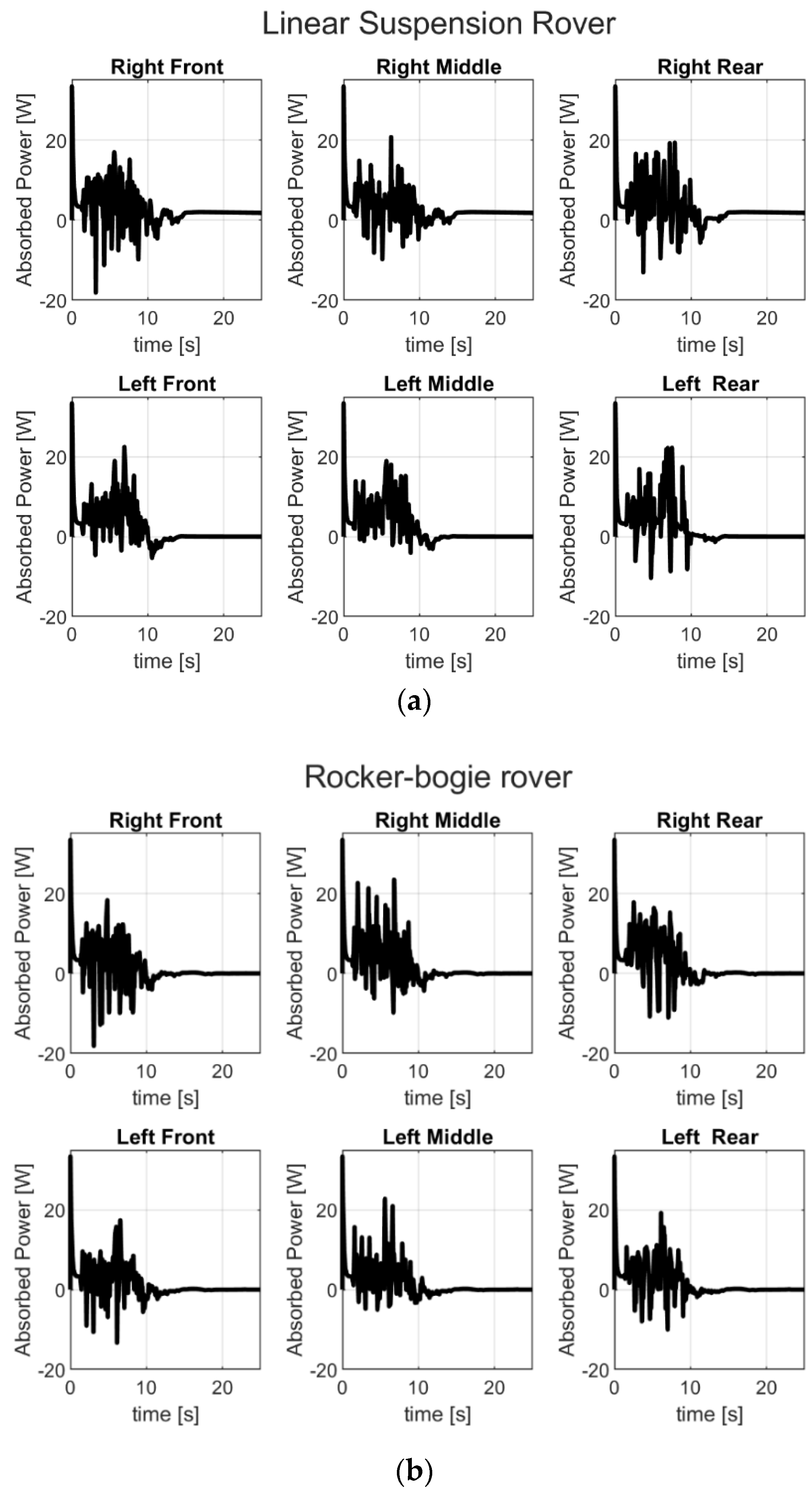
The multibody simulation aided in the evaluation of the energy consumption levels of the two rovers. An interesting aspect was the analysis of the energy absorption starting from power values computed on each wheel motor, as reported in Figure 11.
It is possible to compute the definite integral of the absorbed power values over time for each wheel. The sum of these values returns the absorbed energy in the simulated time.
Table 5 shows energy values for regenerative rates (values labeled with wr subscripts) and non-regenerative rates (values labeled with w/or subscripts) for the two rovers. Energy with regenerative rate accounts even for the negative values of the absorbed power signals given in the above Figure 11. Energyw/or is the integral without considering the regenerative rate (negative part of the integral equal to zero).
Assuming a 12 volt voltage, the battery capacity required for a rover operation time of 40 min can be estimated as:
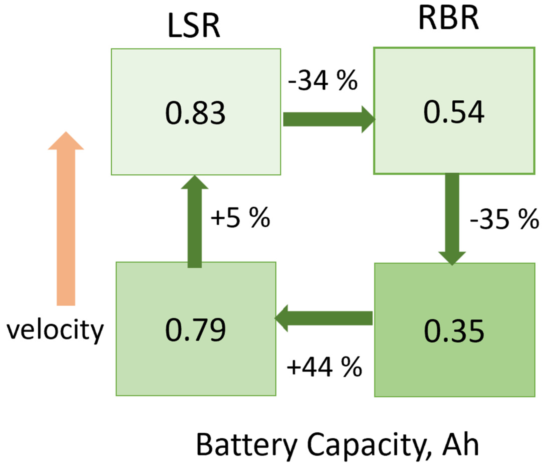
with Energywr values from Table 5 computed over 25 s simulation time. Equation (3) returns a battery capacity of 0.83 Ah for the linear suspension rover and 0.54 Ah for the rocker-bogie rover. This analysis shows an energy savings of 34% for the rocker-bogie rover with respect to the linear suspension rover.
3.3.3. Effect of Lower Velocity on Energy Consumption
An interesting aspect was the evaluation of the effect of velocity on the energy consumption values for both structures. To this end, simulations were carried out at a lower velocity of 1.5 km/h (this value was around 17% less than the velocity set in previous simulations of 1.8 km/h). As reported in Table 6, the energy consumption values for these simulations decreased, as expected, with decreasing velocity.
Figure 12 depicts the differences in energy savings results among the difference simulations when changing the rover structure and vehicle speed. Lower velocity simulations led to energy savings of 44% for the RBR with respect to LSR. The decreased speed returned energy savings of 5% for the LSR and 35% for the RBR. Working at lower speeds with the rocker-bogie rover allowed us to consume half of the energy. This is a remarkable achievement from the point of view of energy savings, especially when considering the applicability of this rover for field operations, such as in agriculture.
4. Conclusions
In this paper, we have shown the development of a multibody simulation test rig for the design of an agricultural rover. The model accounts for contact analysis between the vehicle and ground, as well as for the power electronics. As a case study, we considered two rover structures with the same mass and global envelope, which differed only in their suspension systems. However, the modular structure of the simulation test rig can easily be adapted to study other vehicles.
The simulations allowed the analysis of the main features involved in the design of agricultural rovers.
The rollover study in static conditions is a fundamental aspect, not only to define a rover’s operating conditions in unstructured terrains, but also to evaluate a rover’s safety performance when humans and robotic vehicles have to share the same workspace. The pitch and roll angles guarantee the design-specific features of rovers operating in possible agricultural scenarios, such as vineyards.
Furthermore, the simulations helped to define the motor parameters under critical operating conditions, such as when moving on inclined ground.
The calculated rover dynamics on rough soil allowed an evaluation of suspension the system performance in terms of chassis vibrations and road holdings for both vehicles.
Finally, for the two rover structures travelling at two distinct velocities, a complete overview of the energy saving results has been displayed. This feature makes the created test rig particularly useful for estimating the consumption of these vehicles before they are designed. Indeed, the simulation results showed that the rocker-bogie rover gives an energy saving amount of 34% with respect to the linear Suspension rover under the same operating conditions. The difference in energy savings between the two structures becomes even more pronounced if the rover is operating at lower speeds. The best compromise in terms of energy savings seems to be achieved by the rocker-bogie structure operating at lower speeds. This analysis also allowed us to estimate the battery capacity needed for an operation time of 40 min.
The different aspects analyzed in this study allowed us to define the parameters required for a first protype. Future experimental studies on rover protypes could help validate the simulated results.
For a more accurate design definition, in a future study several aspects must be improved. The model should involve the presence of a fully defined multibody model for the articulated robotic arm. Moreover, the equipment with the vision system could be tested in virtual environments. A further step could be the development of a more accurate contact model between the wheel and the ground. Complex models, for instance, could consider ground in different conditions (wet, snow, mud, and debris). Future studies could even account for embedded sensor systems in the vehicles.
Supplementary Materials
The following materials are available online at https://www.mdpi.com/article/10.3390/machines10040235/s1: Video S1. Linear suspension rover on rough soil. Video S2. Rocker-bogie rover on rough soil. Contact force computations for the six wheels are given in Figures S3 and S4 for the two rover structures.
Author Contributions
Conceptualization, S.S.; methodology, F.C., C.C. and S.S.; software, F.C. and S.S.; validation, F.C., investigation, F.C.; data curation, F.C. and C.C.; writing—original draft preparation, C.C.; writing—review and editing, F.C., C.C., V.N. and S.S.; visualization, F.C. and C.C.; supervision, S.S. and V.N. All authors have read and agreed to the published version of the manuscript.
Funding
This paper received no external funding.
Institutional Review Board Statement
Not applicable.
Informed Consent Statement
Not applicable.
Data Availability Statement
Not applicable.
Acknowledgments
All authors thank Emanuele Della Volpe of Green Tech Solution srl for interesting discussions about the rover design. C.C. and F.C. thank Armando Nicolella for his support in article proofreading. C.C. thanks Ciro Tordela for interesting discussions on the topic.
Conflicts of Interest
The authors declare no conflict of interest.
References
- Liu, Y.; Ma, X.; Shu, L.; Hancke, G.P.; Abu-Mahfouz, A.M. From Industry 4.0 to Agriculture 4.0: Current Status, Enabling Technologies, and Research Challenges. IEEE Trans. Ind. Inform. 2021, 17, 4322–4334. [Google Scholar] [CrossRef]
- Navas, E.; Fernández, R.; Sepúlveda, D.; Armada, M.; Gonzalez-de-Santos, P. Soft Grippers for Automatic Crop Harvesting: A review. Sensors 2021, 21, 2689. [Google Scholar] [CrossRef] [PubMed]
- Friha, O.; Ferrag, M.A.; Shu, L.; Maglaras, L.; Wang, X. Internet of Things for the Future of Smart Agriculture: A Comprehensive Survey of Emerging Technologies. IEEE/CAA J. Autom. Sin. 2021, 8, 718–752. [Google Scholar] [CrossRef]
- Bechar, A.; Vigneault, C. Agricultural robots for field operations: Concepts and components. Biosyst. Eng. 2016, 149, 94–111. [Google Scholar] [CrossRef]
- Kan, X.; Thayer, T.C.; Carpin, S.; Karydis, K. Task Planning on Stochastic Aisle Graphs for Precision Agriculture. IEEE Robot. Autom. Lett. 2021, 6, 3287–3294. [Google Scholar] [CrossRef]
- Cheein, F.A.; Herrera, D.; Gimenez, J.; Carelli, R.; Torres-Torriti, M.; Rosell-Polo, J.R.; Escolà, A.; Arnó, J. Human-robot interaction in precision agriculture: Sharing the workspace with service units. In Proceedings of the 2015 IEEE International Conference on Industrial Technology (ICIT), Seville, Spain, 17–19 March 2015; pp. 289–295. [Google Scholar]
- Silwal, A.; Davidson, J.R.; Karkee, M.; Mo, C.; Zhang, Q.; Lewis, K. Design, integration, and field evaluation of a robotic apple harvester. J. F. Robot. 2017, 34, 1140–1159. [Google Scholar] [CrossRef]
- Bac, C.W.; Hemming, J.; van Tuijl, B.A.J.; Barth, R.; Wais, E.; van Henten, E.J. Performance Evaluation of a Harvesting Robot for Sweet Pepper. J. F. Robot. 2017, 34, 1123–1139. [Google Scholar] [CrossRef]
- Botterill, T.; Paulin, S.; Green, R.; Williams, S.; Lin, J.; Saxton, V.; Mills, S.; Chen, X.Q.; Corbett-Davies, S. A Robot System for Pruning Grape Vines. J. F. Robot. 2017, 34, 1100–1122. [Google Scholar] [CrossRef]
- Bargoti, S.; Underwood, J.P. Image Segmentation for Fruit Detection and Yield Estimation in Apple Orchards. J. F. Robot. 2017, 34, 1039–1060. [Google Scholar] [CrossRef] [Green Version]
- Leonard, E.C. Precision agriculture In Encyclopedia of Food Grains, 2nd ed.; Academic Press: Oxford, UK, 2015; Volume 4, pp. 162–167. [Google Scholar] [CrossRef]
- Stein, M.; Bargoti, S.; Underwood, J. Image Based Mango Fruit Detection, Localisation and Yield Estimation Using Multiple View Geometry. Sensors 2016, 16, 1915. [Google Scholar] [CrossRef]
- Han, J.; Shi, L.; Yang, Q.; Huang, K.; Zha, Y.; Yu, J. Real-time detection of rice phenology through convolutional neural network using handheld camera images. Precis. Agric. 2021, 22, 154–178. [Google Scholar] [CrossRef]
- Koirala, A.; Walsh, K.B.; Wang, Z. Attempting to Estimate the Unseen—Correction for Occluded Fruit in Tree Fruit Load Estimation by Machine Vision with Deep Learning. Agronomy 2021, 11, 347. [Google Scholar] [CrossRef]
- Linaza, M.T.; Posada, J.; Bund, J.; Eisert, P.; Quartulli, M.; Döllner, J.; Pagani, A.; Olaizola, I.G.; Barriguinha, A.; Moysiadis, T.; et al. Data-Driven Artificial Intelligence Applications for Sustainable Precision Agriculture. Agronomy 2021, 11, 1227. [Google Scholar] [CrossRef]
- Bini, D.; Pamela, D.; Prince, S. Machine Vision and Machine Learning for Intelligent Agrobots: A review. In Proceedings of the 2020 5th International Conference on Devices, Circuits and Systems (ICDCS), Coimbatore, India, 5–6 March 2020; pp. 12–16. [Google Scholar]
- Aguiar, A.S.; Dos Santos, F.N.; De Sousa, A.J.M.; Oliveira, P.M.; Santos, L.C. Visual Trunk Detection Using Transfer Learning and a Deep Learning-Based Coprocessor. IEEE Access 2020, 8, 77308–77320. [Google Scholar] [CrossRef]
- Cosenza, C.; Nicolella, A.; Esposito, D.; Niola, V.; Savino, S. Mechanical system control by rgb-d device. Machines 2021, 9, 3. [Google Scholar] [CrossRef]
- Xiong, Y.; Ge, Y.; Grimstad, L.; From, P.J. An autonomous strawberry-harvesting robot: Design, development, integration, and field evaluation. J. F. Robot. 2020, 37, 202–224. [Google Scholar] [CrossRef] [Green Version]
- Auat Cheein, F.A.; Carelli, R. Agricultural robotics: Unmanned robotic service units in agricultural tasks. IEEE Ind. Electron. Mag. 2013, 7, 48–58. [Google Scholar] [CrossRef]
- Mengoli, D.; Tazzari, R.; Marconi, L. Autonomous Robotic Platform for Precision Orchard Management: Architecture and Software Perspective. In Proceedings of the 2020 IEEE International Workshop on Metrology for Agriculture and Forestry (MetroAgriFor), Trento, Italy, 4–6 November 2020; pp. 303–308. [Google Scholar]
- Emmi, L.; Gonzalez-de-Soto, M.; Pajares, G.; Gonzalez-de-Santos, P. Integrating Sensory/Actuation Systems in Agricultural Vehicles. Sensors 2014, 14, 4014–4049. [Google Scholar] [CrossRef]
- Ren, G.; Lin, T.; Ying, Y.; Chowdhary, G.; Ting, K.C. Agricultural robotics research applicable to poultry production: A review. Comput. Electron. Agric. 2020, 169, 105216. [Google Scholar] [CrossRef]
- Fountas, S.; Mylonas, N.; Malounas, I.; Rodias, E.; Hellmann Santos, C.; Pekkeriet, E. Agricultural Robotics for Field Operations. Sensors 2020, 20, 2672. [Google Scholar] [CrossRef]
- Fue, K.G.; Porter, W.M.; Barnes, E.M.; Rains, G.C. An Extensive Review of Mobile Agricultural Robotics for Field Operations: Focus on Cotton Harvesting. AgriEngineering 2020, 2, 150–174. [Google Scholar] [CrossRef] [Green Version]
- Nair, A.S.; Nof, S.Y.; Bechar, A. Emerging Directions of Precision Agriculture and Agricultural Robotics. In Innovation in Agricultural Robotics for Precision Agriculture: A Roadmap for Integrating Robots in Precision Agriculture; Bechar, A., Ed.; Springer International Publishing: Cham, Switzerland, 2021; pp. 177–210. ISBN 978-3-030-77036-5. [Google Scholar]
- Fei, M.; Wendong, H.; Wu, C.; Sai, W. Design and experimental test of multi-functional intelligent vehicle for greenhouse. In Proceedings of the 2021 4th IEEE International Conference on Industrial Cyber-Physical Systems (ICPS), Victoria, BC, Canada, 10–12 May 2021; pp. 755–760. [Google Scholar]
- Bascetta, L.; Baur, M.; Gruosso, G. Electrical Unmanned Vehicle Architecture for Precision Farming Applications. In Proceedings of the 2017 IEEE Vehicle Power and Propulsion Conference (VPPC), Belfort, France, 14–17 December 2017; pp. 1–5. [Google Scholar]
- Hasan, K.M.; Hasan, M.T.; Newaz, S.H.S.; Abdullah-Al-Nahid; Ahsan, M.S. Design and Development of an Autonomous Pesticides Spraying Agricultural Drone. In Proceedings of the 2020 IEEE Region 10 Symposium (TENSYMP), Dhaka, Bangladesh, 5–7 June 2020; pp. 811–814. [Google Scholar]
- Quaglia, G.; Visconte, C.; Scimmi, L.S.; Melchiorre, M.; Cavallone, P.; Pastorelli, S. Design of a UGV powered by solar energy for precision agriculture. Robotics 2020, 9, 13. [Google Scholar] [CrossRef] [Green Version]
- Cavallone, P.; Botta, A.; Carbonari, L.; Visconte, C.; Quaglia, G. The Agri.q Mobile Robot: Preliminary Experimental Tests. In Mechanisms and Machine Science; Springer Nature: Cham, Switzerland, 2021; Volume 91, pp. 524–532. [Google Scholar]
- Nicolini, A.; Mocera, F.; Somà, A. Multibody simulation of a tracked vehicle with deformable ground contact model. Proc. Inst. Mech. Eng. Part K J. Multi-Body Dyn. 2019, 233, 152–162. [Google Scholar] [CrossRef]
- Schafer, B.; Gibbesch, A.; Krenn, R.; Rebele, B. Planetary rover mobility simulation on soft and uneven terrain. In Proceedings of the Vehicle System Dynamics; Taylor & Francis: Abingdon, UK, 2010; Volume 48, pp. 149–169. [Google Scholar]
- Gibbesch, A.; Schäfer, B. Multibody system modelling and simulation of planetary rover mobility on soft terrain. In Proceedings of the 8th International Symposium on Artifical Intelligence, Robotics and Automation in Space—iSAIRAS, Munich, Germany, 5–8 September 2005; pp. 105–112. [Google Scholar]
- Nayar, H.; Kim, J.; Chamberlain-Simon, B.; Carpenter, K.; Hans, M.; Boettcher, A.; Meirion-Griffith, G.; Wilcox, B.; Bittner, B. Design optimization of a lightweight rocker–bogie rover for ocean worlds applications. Int. J. Adv. Robot. Syst. 2019, 16. [Google Scholar] [CrossRef]
- Wang, G.; Yu, Y.; Feng, Q. Design of End-effector for Tomato Robotic Harvesting. In Proceedings of the IFAC-PapersOnLine; Elsevier B.V.: Amsterdam, The Netherlands, 2016; Volume 49, pp. 190–193. [Google Scholar]
- Han, J.B.; Yang, K.M.; Kim, D.H.; Seo, K.H. A Modeling and Simulation based on the Multibody Dynamics for an Autonomous Agricultural Robot. In Proceedings of the 2019 IEEE 7th International Conference on Control, Mechatronics and Automation, ICCMA 2019, Delft, The Netherlands, 6–8 November 2019; pp. 137–143. [Google Scholar]
- Cosenza, C.; Niola, V.; Savino, S. Underactuated finger behavior correlation between vision system based experimental tests and multibody simulations. In Mechanisms and Machine Science; Springer Nature: Cham, Switzerland, 2019; Volume 66, pp. 49–56. [Google Scholar]
- Melzi, S.; Sabbioni, E.; Vignati, M.; Cutini, M.; Brambilla, M.; Bisaglia, C.; Cavallo, E. Multibody model of fruit harvesting trucks: Comparison with experimental data and rollover analysis. J. Agric. Eng. 2018, 49, 92–99. [Google Scholar] [CrossRef] [Green Version]
- Calli, B.; Dollar, A.M. Vision-based model predictive control for within-hand precision manipulation with underactuated grippers. In Proceedings of the IEEE International Conference on Robotics and Automation, Singapore, 29 May–3 June 2017; pp. 2839–2845. [Google Scholar]
- Cosenza, C.; Niola, V.; Savino, S. A simplified model of a multi-jointed mechanical finger calibrated with experimental data by vision system. Proc. Inst. Mech. Eng. Part K J. Multi-Body Dyn. 2021, 235, 164–175. [Google Scholar] [CrossRef]
- Brancati, R.; Cosenza, C.; Niola, V.; Savino, S. Experimental measurement of underactuated robotic finger configurations via RGB-D sensor. In Mechanisms and Machine Science; Springer Nature: Cham, Switzerland, 2019; Volume 67, pp. 531–537. [Google Scholar]
- Harrington, B.D.; Voorhees, C. The Challenges of Designing the Rocker-Bogie Suspension for the Mars Exploration Rover. In Proceedings of the 37th Aerospace Mechanisms Symposium, Johnson Space Center, Houston, TX, USA, 19–21 May 2004; pp. 185–195. [Google Scholar]
- Bickler, D.B. Articulated Suspension System. U.S. Patent 4,840,394, 6 January 1989. [Google Scholar]
Figure 1.
Main blocks composing the multibody simulation test rig for the agricultural rover design.
Figure 1.
Main blocks composing the multibody simulation test rig for the agricultural rover design.

Figure 2.
Rover vehicle structures used in this paper: the linear suspension rover (LSR) (a) equipped with two independent spring–damper suspension systems; (b) the rocker-bogie rover (RBR), which employs an articulated suspension system similar to the rover used for Mars exploration.
Figure 2.
Rover vehicle structures used in this paper: the linear suspension rover (LSR) (a) equipped with two independent spring–damper suspension systems; (b) the rocker-bogie rover (RBR), which employs an articulated suspension system similar to the rover used for Mars exploration.

Figure 3.
The main parameters of the control strategy.

Figure 4.
Example of input voltages to the right and left sides for rover control.

Figure 5.
Displacement, velocity, and acceleration profiles for inverse dynamics simulations.

Figure 6.
Multibody simulation of the rover in static conditions for the rollover study. Roll and pitch angle variations were considered for this first test.
Figure 6.
Multibody simulation of the rover in static conditions for the rollover study. Roll and pitch angle variations were considered for this first test.

Figure 7.
Torque values computed on right-side wheels in inverse dynamics simulations.

Figure 8.
Direct dynamics simulation on rough soil: (a) LSR; (b) RBR.

Figure 9.
Vibration analysis in terms of acceleration signals: (a) LSR; (b) RBR.

Figure 10.
Contact force between the wheel and ground for the left rear wheel: (a) LSR; (b) RBR.

Figure 11.
Absorbed power on the motor of each wheel: (a) linear suspension rover; (b) rocker-bogie rover.
Figure 11.
Absorbed power on the motor of each wheel: (a) linear suspension rover; (b) rocker-bogie rover.

Figure 12.
Energy saving results in terms of battery capacity estimations for the two rover structures moving at two different speeds.
Figure 12.
Energy saving results in terms of battery capacity estimations for the two rover structures moving at two different speeds.


Table 1.
Multibody simulation details.
| Rover Design | Type | Soil | Integrator | Step | Output |
|---|---|---|---|---|---|
| Rollover study | Inverse dynamics | Smooth | Ode23t (mod. Stiff/Trapezoidal) | Variable-step | Pitch and Roll angles |
| Motor sizing | Inverse dynamics | Smooth | Ode23t (mod. Stiff/Trapezoidal) | Variable-step | Drive Torques |
| Suspension performance | Direct dynamics | Rough | Ode23t (mod. Stiff/Trapezoidal) | Variable-step | Chassis Vibrations, Contact Force 1 |
| Energy Consumption | Direct dynamics | Rough | Ode23t (mod. Stiff/Trapezoidal) | Variable-step | Absorbed Power |
1 Estimated between wheel and ground.
Table 2.
Rollover study results for maximum pitch and roll angles 1.
| Pitch | Roll | |
|---|---|---|
| Linear suspension rover | 41 | 45 |
| Rocker-bogie rover | 45 | 37 |
1 Angles are reported in degrees.
Table 3.
DC motor parameters set in direct dynamics simulations.
| Nominal voltage | 12 V |
| Transmission ratio | 1/90 |
| Idle Velocity | 180 rpm |
| Idle current | ≤1.1 A |
| Nominal Torque | 2.647 Nm |
| Nominal velocity | 120 rpm |
| Nominal current | ≤6 A |
Table 4.
Duration for which the contact force was equal to zero.
| Wheel | Right Front | Right Middle | Right Rear | Left Front | Left Middle | Left Rear |
|---|---|---|---|---|---|---|
| Linear suspension rover | 1.59 | 2.06 | 4.04 | 0.80 | 1.96 | 4.16 |
| Rocker-bogie rover | 0.49 | 0.18 | 0.88 | 0.09 | 0.20 | 0.71 |
Table 5.
Energy 1 consumption.
| Energywr [J] | Battery 2wr Capacity [Ah] | Energyw/or [J] | Battery 2w/or Capacity [Ah] | |
|---|---|---|---|---|
| Linear suspension rover | 3.74 × 10² | 0.83 | 4.08 × 10² | 0.91 |
| Rocker-bogie rover | 2.45 × 10² | 0.54 | 2.91 × 10² | 0.65 |
1 Over a simulation time of 25 s; 2 assuming 12 V voltage.
Table 6.
Energy 1 consumption levels at lower velocity.
| Energywr [J] | Battery 2wr Capacity [Ah] | Energyw/or [J] | Battery 2w/or Capacity [Ah] | |
|---|---|---|---|---|
| Linear suspension rover | 3.54 × 10² | 0.79 | 3.91 × 10² | 0.87 |
| Rocker-bogie rover | 1.59 × 10² | 0.35 | 2.03 × 10² | 0.45 |
1 Over a simulation time of 25 s; 2 assuming 12 V voltage.
Publisher’s Note: MDPI stays neutral with regard to jurisdictional claims in published maps and institutional affiliations. |
© 2022 by the authors. Licensee MDPI, Basel, Switzerland. This article is an open access article distributed under the terms and conditions of the Creative Commons Attribution (CC BY) license (https://creativecommons.org/licenses/by/4.0/).
Share and Cite
MDPI and ACS Style
Califano, F.; Cosenza, C.; Niola, V.; Savino, S. Multibody Model for the Design of a Rover for Agricultural Applications: A Preliminary Study. Machines 2022, 10, 235. https://doi.org/10.3390/machines10040235
AMA Style
Califano F, Cosenza C, Niola V, Savino S. Multibody Model for the Design of a Rover for Agricultural Applications: A Preliminary Study. Machines. 2022; 10(4):235. https://doi.org/10.3390/machines10040235
Chicago/Turabian StyleCalifano, Filippo, Chiara Cosenza, Vincenzo Niola, and Sergio Savino. 2022. "Multibody Model for the Design of a Rover for Agricultural Applications: A Preliminary Study" Machines 10, no. 4: 235. https://doi.org/10.3390/machines10040235
Note that from the first issue of 2016, this journal uses article numbers instead of page numbers. See further details here.