A Variable-Length Rational Finite Element Based on the Absolute Nodal Coordinate Formulation

Abstract

The variable-length arbitrary Lagrange–Euler absolute nodal coordinate formulation (ALE-ANCF) finite element, which employs nonrational interpolating polynomials, cannot exactly describe rational cubic Bezier curves such as conic and circular curves. The rational absolute nodal coordinate formulation (RANCF) finite element, whose reference length (undeformed length) is constant, can exactly represent rational cubic Bezier curves. A new variable-length finite element called the ALE-RANCF finite element, which is capable of accurately describing rational cubic Bezier curves, is proposed and was formed by combining the desirable features of the ALE-ANCF and RANCF finite elements. To control the reference length of the ALE-RANCF element within a suitable range, element segmentation and merging schemes are proposed. It is demonstrated that the exact geometry and mechanics are maintained after the ALE-RANCF element is divided into two shorter ones, and compared with the ALE-ANCF elements, there are smaller deviations and oscillations after two ALE-RANCF elements are merged into a longer one. Numerical examples are presented, and the feasibility and advantages of the ALE-RANCF finite element are demonstrated.

1. Introduction

The sliding joint on a flexible beam [1,2,3,4] is widely used in the dynamic modeling of practical engineering systems, such as pantograph/catenary systems [5,6], tethered satellite systems [7,8], and arresting systems [9]. The variable-length arbitrary Lagrange–Euler absolute nodal coordinate formulation (ALE-ANCF) finite element [10,11], which can be used to efficiently and effectively implement the sliding joint dynamic model, was established based on absolute nodal coordinate formulation (ANCF) [12,13,14,15,16] in the framework of the arbitrary Lagrange–Euler (ALE) description. The material coordinates of the nodal point are adopted as generalized coordinates in the ALE formulation to enable the length variation of the ALE-ANCF element. The ALE-ANCF sliding joint is implemented by positing the coupling point at a moving node on the axis of the beam, which is realized by changing the length of the two adjacent elements of the sliding joint in a conjugate manner. The ALE-ANCF was successfully used in the dynamic modeling of tethered satellite systems [7,8], arresting systems [9], and cable–pulley systems [17,18,19], and its feasibility was demonstrated. Nonrational functions cannot be used to exactly represent some geometric shapes such as conic and circular shapes; therefore, the ALE-ANCF beam elements that employ nonrational interpolating polynomials cannot exactly describe conic and circular curves. This problem can be solved by substituting the nonrational interpolating polynomials with rational interpolating polynomials, which were used in the rational absolute nodal coordinate formulation (RANCF) finite elements [20,21,22,23,24].

Hughes et al. [25] pointed out that the geometric description methods of computer-aided design (CAD) and conventional computer-aided analysis (CAA) are inconsistent; consequently, the construction of finite element geometry (i.e., the mesh) is costly and time-consuming and creates inaccuracies. The nonuniform rational B-splines (NURBS) [26] curve, which is a standard technology employed in CAD systems, can be systematically and linearly transformed into a series of RANCF finite elements [20,21]. The RANCF finite elements, which employ rational interpolating polynomials, can exactly describe the rational cubic Bezier curves and facilitate the integration of computer-aided design and analysis (ICADA) [27]. The primary aim of this work is to combine the desirable features of the ALE-ANCF finite elements and the RANCF finite elements to establish a new variable-length ALE-RANCF finite element that could accurately capture rational cubic Bezier geometric shapes.

The second aim of this study is to propose an element length-control scheme to control the reference length of the ALE-RANCF element within a suitable range. The accuracy of the simulation will decrease if the element length becomes too long [10]. The element mass matrix will become singular and ill-conditioned, and the numerical integration will be flawed, if the element length becomes too short [10]. In a practical simulation, a new node could be inserted into the element to divide it into two shorter elements if the element is longer than the prescribed threshold. By contrast, a node could be removed to merge the element with its neighbor to form a new longer element if the element is shorter than the prescribed threshold. It is demonstrated that the exact geometry and mechanic are maintained after the ALE-RANCF element is segmented, and compared with that of ALE-ANCF elements, there are smaller deviations and vibrations after two ALE-RANCF elements are merged.

The third aim of this work is to develop dynamic model of sliding joint on a Euler–Bernoulli beam [28] using the ALE-RANCF finite elements. Three numerical examples are presented to demonstrate the feasibility and advantages of the ALE-RANCF finite elements. The rest of this paper is organized as follows. In Section 2, a brief review of the RANCF finite element is presented, and some fundamental concepts and equations that are repeatedly used in the following sections are introduced. The ALE-RANCF finite element is established and its governing equation is derived in Section 3. In Section 4, the ALE-RANCF element length-control scheme is proposed, including the element segmentation and merging scheme. A dynamic model of the sliding joint is established in Section 5. Numerical examples are described, and the results are discussed in Section 6. A summary and the conclusions drawn from this study are presented in Section 7.

2. RANCF Finite Element

In this section, a brief review of the RANCF finite element model and some fundamental concepts and equations that are repeatedly used in this paper are introduced. A simple Euler–Bernoulli beam [28] whose geometric shape and displacement field only depend on its material coordinate is adopted as an example. The RANCF finite element was derived by integrating the NURBS geometry and the ANCF finite elements. A NURBS curve can be converted into a series of rational Bezier curves and such a conversion preserves the exact geometry of the curve [26]. The displacement field of a Bezier curve with n-degree is defined as:

$$\mathbf{r}\left(u\right)=\sum _{i=0}^n{R}_{i,n}\left(u\right){\mathbf{P}}_i,0\le u\le 1$$

(1)

In this equation, $\mathbf{r}\left(u\right)$ is the position of any arbitrary point on curve, the coefficient ${\mathbf{P}}_i$ are control points, and the basis functions $R_{i,n}\left(u\right)$ are defined as:

$$R_{i,n}\left(u\right)=\frac{w_i{B}_{i,n}\left(u\right)}{{\sum }_{i=0}^n{w}_i{B}_{i,n}\left(u\right)}$$

(2)

where $w_i>0$ are the weights, $B_{i,n}\left(u\right)$ are the n-degree Bernstein polynomials defined as:

$$B_{i,n}\left(u\right)=\frac{n!}{i!(n-i)!}{u}^i{(1-u)}^{n-i}$$

(3)

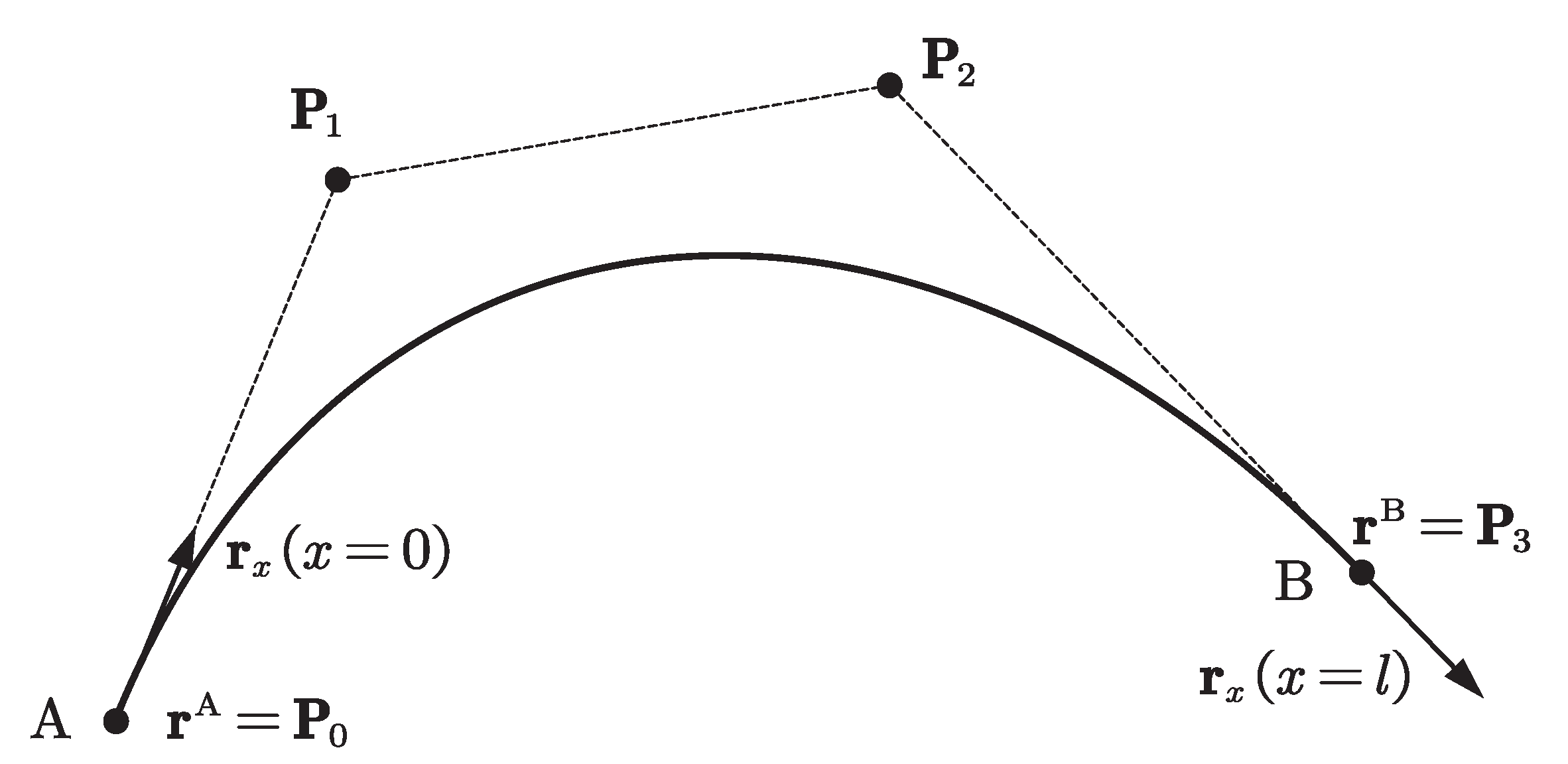
The rational cubic Bezier curve coordinates can be linearly transformed to the RANCF form [20]. The RANCF element nodal coordinate vector is defined as:

$$\mathbf{e}={\left[\begin{array}{cccc}{\left({\mathbf{r}}^{\mathrm{A}}\right)}^{\mathrm{T}}& {\left({\mathbf{r}}_x^{\mathrm{A}}\right)}^{\mathrm{T}}& {\left({\mathbf{r}}^{\mathrm{B}}\right)}^{\mathrm{T}}& {\left({\mathbf{r}}_x^{\mathrm{B}}\right)}^{\mathrm{T}}\end{array}\right]}^{\mathrm{T}}$$

(4)

where ${\mathbf{r}}^{\mathrm{N}},\mathrm{N}=\mathrm{A}\mathrm{or}\mathrm{B}$ are the nodal position coordinates, the superscripts A and B refer to the start and end nodes of element AB as shown in Figure 1, ${\mathbf{r}}_x^{\mathrm{N}}=\partial {\mathbf{r}}^{\mathrm{N}}/\partial x$ are the nodal position coordinate gradients, and x is the material coordinate. Assuming $u=x/l$, where l is the reference length of the element. The transformation from the rational cubic Bezier curve control points to the RANCF element coordinates [20] can be formulated as:

$$\left[\begin{array}{c}{\mathbf{r}}^{\mathrm{A}}\\ {\mathbf{r}}_x^{\mathrm{A}}\\ {\mathbf{r}}^{\mathrm{B}}\\ {\mathbf{r}}_x^{\mathrm{B}}\end{array}\right]=\left[\begin{array}{c}{\mathbf{P}}_0\\ {\displaystyle \frac{3w_1}{l{w}_0}}({\mathbf{P}}_1-{\mathbf{P}}_0)\\ {\mathbf{P}}_3\\ {\displaystyle \frac{3w_2}{l{w}_3}}({\mathbf{P}}_3-{\mathbf{P}}_2)\end{array}\right]$$

(5)

The inverse transformation can be written in a matrix form as:

$$\left[\begin{array}{c}{\mathbf{P}}_0\\ {\mathbf{P}}_1\\ {\mathbf{P}}_2\\ {\mathbf{P}}_3\end{array}\right]=\left[\begin{array}{cccc}\mathbf{I}& \mathbf{0}& \mathbf{0}& \mathbf{0}\\ \mathbf{I}& {\displaystyle \frac{l{w}_0}{3w_1}}\mathbf{I}& \mathbf{0}& \mathbf{0}\\ \mathbf{0}& \mathbf{0}& \mathbf{I}& -{\displaystyle \frac{l{w}_3}{3w_2}}\mathbf{I}\\ \mathbf{0}& \mathbf{0}& \mathbf{I}& \mathbf{0}\end{array}\right]\left[\begin{array}{c}{\mathbf{r}}^{\mathrm{A}}\\ {\mathbf{r}}_x^{\mathrm{A}}\\ {\mathbf{r}}^{\mathrm{B}}\\ {\mathbf{r}}_x^{\mathrm{B}}\end{array}\right]$$

(6)

where $\mathbf{I}$ is the identity matrix. By substituting Equation (6) into the Bezier curve expression Equation (1), the displacement field of the RANCF finite element [20] can be written as:

$$\mathbf{r}\left(u,t\right)=\mathbf{S}\left(u\right)\mathbf{e}\left(t\right)$$

(7)

In this equation, $\mathbf{e}\left(t\right)$ is the element nodal coordinate vector at time t, $\mathbf{S}\left(u\right)$ is the shape function matrix, where:

$$\mathbf{S}\left(u\right)=\left[\begin{array}{cccc}{s}_1\left(u\right)\mathbf{I}& s_2\left(u\right)\mathbf{I}& s_3\left(u\right)\mathbf{I}& s_4\left(u\right)\mathbf{I}\end{array}\right]$$

(8)

where

$$\begin{array}{c}\left[\begin{array}{c}{s}_1\left(u\right)\\ s_2\left(u\right)\\ s_3\left(u\right)\\ s_4\left(u\right)\end{array}\right]=\left[\begin{array}{c}{R}_{0,3}+R_{1,3}\\ {\displaystyle \frac{l{w}_0}{3w_1}}{R}_{1,3}\\ R_{2,3}+R_{3,3}\\ -{\displaystyle \frac{l{w}_3}{3w_2}}{R}_{2,3}\end{array}\right]={\displaystyle \frac{1}{W\left(u\right)}}\left[\begin{array}{c}3w_{1}u{(1-u)}^2+w_0{(1-u)}^3\\ l{w}_{0}u{(1-u)}^2\\ w_3{u}^3+3w_2{u}^2(1-u)\\ -l{w}_3{u}^2(1-u)\end{array}\right]\\ W\left(u\right)=w_3{u}^3+3w_2{u}^2\left(1-u\right)+3w_{1}u{\left(1-u\right)}^2+w_0{\left(1-u\right)}^3>0\end{array}$$

(9)

Different from the nonrational polynomial shape functions of the conventional ANCF elements, the RANCF element shape functions are rational polynomials. Assuming all the weight coefficients of the RANCF elements are equal, then new shape functions can be obtained as:

$$\begin{array}{cc}{s}_1\left(u\right)=1-3u^2+2u^3,\hfill & s_2\left(u\right)=l(u-2u^2+u^3)\hfill \\ s_3\left(u\right)=3u^2-2u^3,\hfill & s_4\left(u\right)=l(-u^2+u^3)\hfill \end{array}$$

(10)

This is exactly the same as shape functions of the conventional ANCF element [29,30]. Hence, one can say that the conventional ANCF element is a special case of the RANCF element.

Although the weights have a direct effect on the geometric shapes and properties of the RANCF element, the weights are treated as the inherent attribute parameters rather than the additional degree of freedom, of the element. This is because the RANCF finite element is an estimation rather than an accurate description of the deformed element, and treating the weights as the degrees of freedom of the elements will only increase the complexity of the dynamic model. Furthermore, using the constant weights assumption, all the desirable features of the ANCF finite elements can be retained for the RANCF finite elements, including the constant mass matrix and the zero Coriolis and centrifugal forces.

3. ALE-RANCF Finite Element

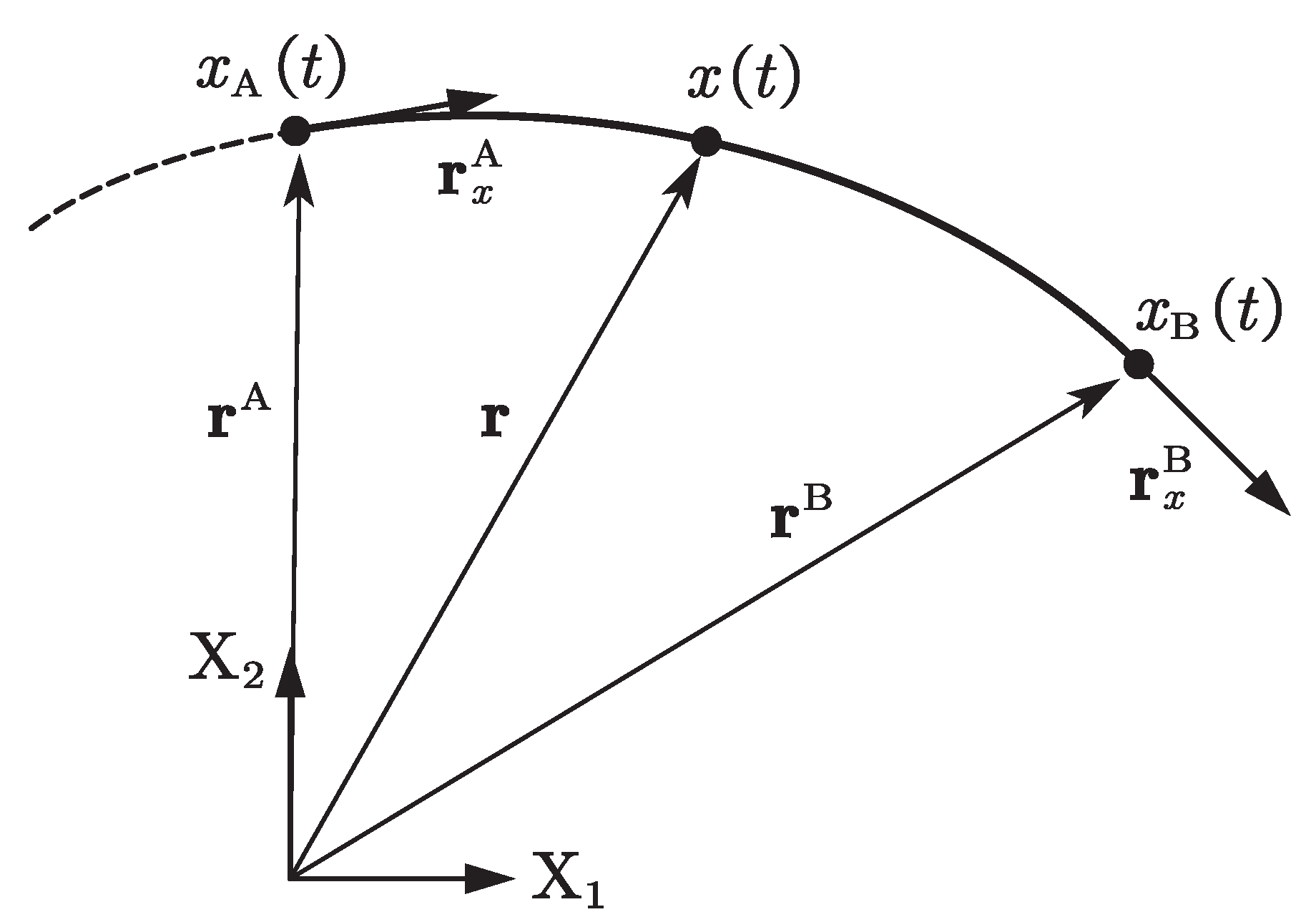
The variable-length ALE-RANCF finite element (Figure 2) will be proposed in this section. To enable the length variation of the RANCF finite element, the nodal material parameters $x_{\mathrm{A}}$, $x_{\mathrm{B}}$, which denote the length from material points A and B to head point of the beam in undeformed configuration, are employed as the generalized coordinates [10]. By combining the nodal position coordinates, the nodal position coordinate gradients, and the nodal material coordinates of the element, the generalized coordinate vector of the ALE-RANCF finite element can be defined as:

$$\mathbf{q}={\left[\begin{array}{cccccc}{\left({\mathbf{r}}^{\mathrm{A}}\right)}^{\mathrm{T}}& {\left({\mathbf{r}}_x^{\mathrm{A}}\right)}^{\mathrm{T}}& {\left({\mathbf{r}}^{\mathrm{B}}\right)}^{\mathrm{T}}& {\left({\mathbf{r}}_x^{\mathrm{B}}\right)}^{\mathrm{T}}& x_{\mathrm{A}}\left(t\right)& x_{\mathrm{B}}\left(t\right)\end{array}\right]}^{\mathrm{T}}$$

(11)

The displacement field of the ALE-RANCF finite element can be written as:

$$\mathbf{r}(x,t)=\mathbf{S}\left(x,x_{\mathrm{A}}\left(t\right),x_{\mathrm{B}}\left(t\right)\right)\mathbf{e}\left(t\right)$$

(12)

where $\mathbf{S}\left(x,x_{\mathrm{A}}\left(t\right),x_{\mathrm{B}}\left(t\right)\right)$ is the shape function matrix of the ALE-RANCF element, which can be obtained by make the substitutions

$$u=\frac{x-x_{\mathrm{A}}\left(t\right)}{x_{\mathrm{B}}\left(t\right)-x_{\mathrm{A}}\left(t\right)},l=x_{\mathrm{B}}\left(t\right)-x_{\mathrm{A}}\left(t\right)$$

(13)

for RANCF element shape functions (Equation (9)).

The expressions of velocity $\dot{\mathbf{r}}$, acceleration $\ddot{\mathbf{r}}$, as well as displacement variation $\delta \mathbf{r}$, of the point in the ALE-RANCF element, which will be used in deriving the element governing equation, can be formulated in matrix form as:

$$\dot{\mathbf{r}}=\mathbf{N}\dot{\mathbf{q}},\ddot{\mathbf{r}}=\mathbf{N}\ddot{\mathbf{q}}+{\mathbf{r}}_v,\delta \mathbf{r}=\mathbf{N}\delta \mathbf{q}$$

(14)

where

$$\begin{array}{c}\mathbf{N}=\left[\begin{array}{ccc}\mathbf{S}& {\displaystyle \frac{\partial \mathbf{S}}{\partial x_{\mathrm{A}}}}\mathbf{e}& {\displaystyle \frac{\partial \mathbf{S}}{\partial x_{\mathrm{B}}}}\mathbf{e}\end{array}\right]\\ {\mathbf{r}}_v=2\left({\displaystyle \frac{\partial \mathbf{S}}{\partial x_{\mathrm{A}}}}{\dot{x}}_{\mathrm{A}}+{\displaystyle \frac{\partial \mathbf{S}}{\partial x_{\mathrm{B}}}}{\dot{x}}_{\mathrm{B}}\right)\dot{\mathbf{e}}+\left({\displaystyle \frac{{\partial }^2\mathbf{S}}{\partial x_{\mathrm{A}}^2}}{\dot{x}}_{\mathrm{A}}^2+2{\displaystyle \frac{{\partial }^2\mathbf{S}}{\partial x_{\mathrm{A}}\partial x_{\mathrm{B}}}}{\dot{x}}_{\mathrm{A}}{\dot{x}}_{\mathrm{B}}+{\displaystyle \frac{{\partial }^2\mathbf{S}}{\partial x_{\mathrm{B}}^2}}{\dot{x}}_{\mathrm{B}}^2\right)\mathbf{e}\end{array}$$

(15)

According to the virtual work principle, one can obtain that:

$$\delta W_{\mathrm{m}}+\delta W_{\mathrm{l}}+\delta W_{\mathrm{t}}+\delta W_{\mathrm{g}}=0$$

(16)

where $\delta W_{\mathrm{m}}$ is the virtual work of the element inertia force, $\delta W_{\mathrm{l}}$ and $\delta W_{\mathrm{t}}$ are the virtual work of the element elastic force due to the longitudinal and transverse deformation respectively, and $\delta W_{\mathrm{g}}$ is the virtual work of the element gravity. The virtual works can be formulated as:

$${\displaystyle \left\{{\displaystyle \begin{array}{c}\begin{array}{c}{\displaystyle \delta W_{\mathrm{m}}={\int }_{x_{\mathrm{A}}}^{x_{\mathrm{B}}}\delta {\mathbf{r}}^{\mathrm{T}}\left(-\rho A\ddot{\mathbf{r}}\right)\mathrm{d}x=\delta {\mathbf{q}}^{\mathrm{T}}\left(-\mathbf{M}\ddot{\mathbf{q}}-{\mathbf{Q}}_{\mathrm{a}}\right)}\hfill \end{array}\\ \delta W_{\mathrm{l}}={\int }_{x_{\mathrm{A}}}^{x_{\mathrm{B}}}-\delta {\epsilon }_{0}EA\left({\epsilon }_0+c{\dot{\epsilon }}_0\right)\mathrm{d}x=\delta {\mathbf{q}}^{\mathrm{T}}(-{\mathbf{Q}}_{\mathrm{l}})\\ \delta W_{\mathrm{t}}={\int }_{x_{\mathrm{A}}}^{x_{\mathrm{B}}}-\delta \kappa EI\left(\kappa +c\dot{\kappa }\right)\mathrm{d}x=\delta {\mathbf{q}}^{\mathrm{T}}(-{\mathbf{Q}}_{\mathrm{t}})\\ \delta W_{\mathrm{g}}={\int }_{x_{\mathrm{A}}}^{x_{\mathrm{B}}}\delta {\mathbf{r}}^{\mathrm{T}}\left(\rho A\mathbf{g}\right)\mathrm{d}x=\delta {\mathbf{q}}^{\mathrm{T}}{\mathbf{Q}}_{\mathrm{g}}\end{array}}\right.}$$

(17)

By substituting Equation (17) into Equation (16), the dynamic equations of motion without the constraint forces can be obtained as:

$$\mathbf{M}\ddot{\mathbf{q}}+{\mathbf{Q}}_{\mathrm{a}}+{\mathbf{Q}}_{\mathrm{l}}+{\mathbf{Q}}_{\mathrm{t}}-{\mathbf{Q}}_{\mathrm{g}}=\mathbf{0}$$

(18)

where $\mathbf{M}$ is the element mass matrix, ${\mathbf{Q}}_{\mathrm{a}}$ is the generalized additional inertia force due to the time-variation of the material coordinates, ${\mathbf{Q}}_{\mathrm{l}}$ and ${\mathbf{Q}}_{\mathrm{t}}$ are the generalized elastic forces due to the longitudinal and transverse deformation, respectively, and ${\mathbf{Q}}_{\mathrm{g}}$ is the generalized gravitational force. The mass matrix and generalized forces of the ALE-RANCF element can be formulated as:

$${\displaystyle \left\{\begin{array}{c}\begin{array}{c}{\displaystyle \mathbf{M}={\int }_{x_{\mathrm{A}}}^{x_{\mathrm{B}}}\rho A{\mathbf{N}}^{\mathrm{T}}\mathbf{N}\mathrm{d}x=\rho Al{\int }_0^1{\mathbf{N}}^{\mathrm{T}}\mathbf{N}\mathrm{d}u}\hfill \end{array}\\ {\mathbf{Q}}_{\mathrm{a}}={\int }_{x_{\mathrm{A}}}^{x_{\mathrm{B}}}\rho A{\mathbf{N}}^{\mathrm{T}}{\mathbf{r}}_v\mathrm{d}x=\rho Al{\int }_0^1{\mathbf{N}}^{\mathrm{T}}{\mathbf{r}}_v\mathrm{d}u\\ {\mathbf{Q}}_{\mathrm{l}}={\int }_{x_{\mathrm{A}}}^{x_{\mathrm{B}}}{\left({\displaystyle \frac{\partial \epsilon }{\partial \mathbf{q}}}\right)}^{\mathrm{T}}EA\left(\epsilon +c\dot{\epsilon }\right)\mathrm{d}x=EAl{\int }_0^1{\left({\displaystyle \frac{\partial \epsilon }{\partial \mathbf{q}}}\right)}^{\mathrm{T}}\left(\epsilon +c\dot{\epsilon }\right)\mathrm{d}u\\ {\mathbf{Q}}_{\mathrm{t}}={\int }_{x_{\mathrm{A}}}^{x_{\mathrm{B}}}{\left({\displaystyle \frac{\partial \kappa }{\partial \mathbf{q}}}\right)}^{\mathrm{T}}EI\left(\kappa +c\dot{\kappa }\right)\mathrm{d}x=EIl{\int }_0^1{\left({\displaystyle \frac{\partial \kappa }{\partial \mathbf{q}}}\right)}^{\mathrm{T}}\left(\kappa +c\dot{\kappa }\right)\mathrm{d}u\\ {\mathbf{Q}}_{\mathrm{g}}={\int }_{x_{\mathrm{A}}}^{x_{\mathrm{B}}}{\mathbf{N}}^{\mathrm{T}}\left(\rho A\mathrm{g}\right)dx=\rho Al{\int }_1^0{\mathbf{N}}^{\mathrm{T}}\mathrm{g}\mathrm{d}u\end{array}\right.}$$

(19)

In this equation, $\rho$ is the beam density, A is the beam cross section area, E is the Young’s modulus, I is the second area of moment, c is the damping coefficient, $\mathbf{g}$ is the gravitational acceleration vector in global coordinate system, $\epsilon =\left({\mathbf{r}}_x^{\mathrm{T}}{\mathbf{r}}_x-1\right)/2$ is the Cauchy–Green longitudinal strain, and $\kappa =\left|{\mathbf{r}}_x\times {\mathbf{r}}_{xx}\right|/{\left|{\mathbf{r}}_x\right|}^3$ is the curvature. The expressions of the longitudinal strain and curvature were derived in literature [29].

By using the method of Lagrange multipliers to introduce the virtual work of the constraints’ forces, the governing equation of the ALE-RANCF element can be given as:

$$\mathbf{M}\ddot{\mathbf{q}}+{\mathbf{C}}_{\mathbf{q}}^{\mathrm{T}}\lambda +\mathbf{Q}\left(\dot{\mathbf{q}},\mathbf{q},t\right)=\mathbf{0}$$

(20)

where ${\mathbf{C}}_{\mathbf{q}}=\partial \mathbf{C}/\partial \mathbf{q}$ is the Jacobian matrix of the constraints, $\lambda$ is the vector of Lagrange multipliers, and $\mathbf{Q}\left(\dot{\mathbf{q}},\mathbf{q},t\right)$ is the generalized force vector consist of additional inertia force, elastic force, and gravitational force, respectively.

4. Element Length Control

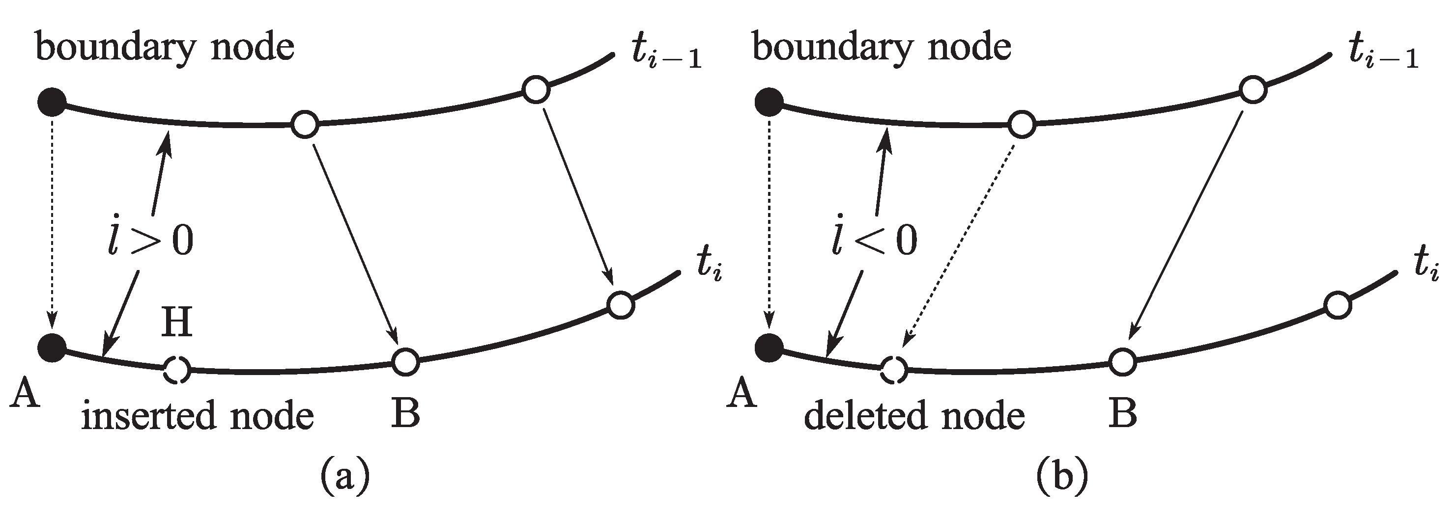
As mentioned in the introduction Section 1, too long or too short element length will reduce the accuracy of the dynamic model in practical simulation; therefore, it is important to control the reference length of the ALE-RANCF element within a suitable range. A length-control scheme for the ALE-ANCF element was introduced in reference [10]. A new node can be inserted into the element to divide it into two shorter ones if the element is longer than the prescribed threshold (Figure 3a). In contrast, a node can be removed to merge the element with its neighbor to form a new longer element if the element is short than the prescribed threshold (Figure 3b).

The segmentation of the element increases the degree of freedom of the dynamic model. It will be demonstrated that the element segmentation scheme introduced in this section maintains exact geometry and mechanic, although the weights and shape functions of the elements will be changed after the ALE-RANCF element is segmented. While the merging of the element decreases the degree of freedom of the dynamic model, as a result, the geometric and mechanical deviation will be inevitable. However, it will be demonstrated that compared with the ALE-ANCF, the deviations and vibrations of the ALE-RANCF elements could be reduced by adjusting the weights of the merged element.

4.1. Element Segmentation

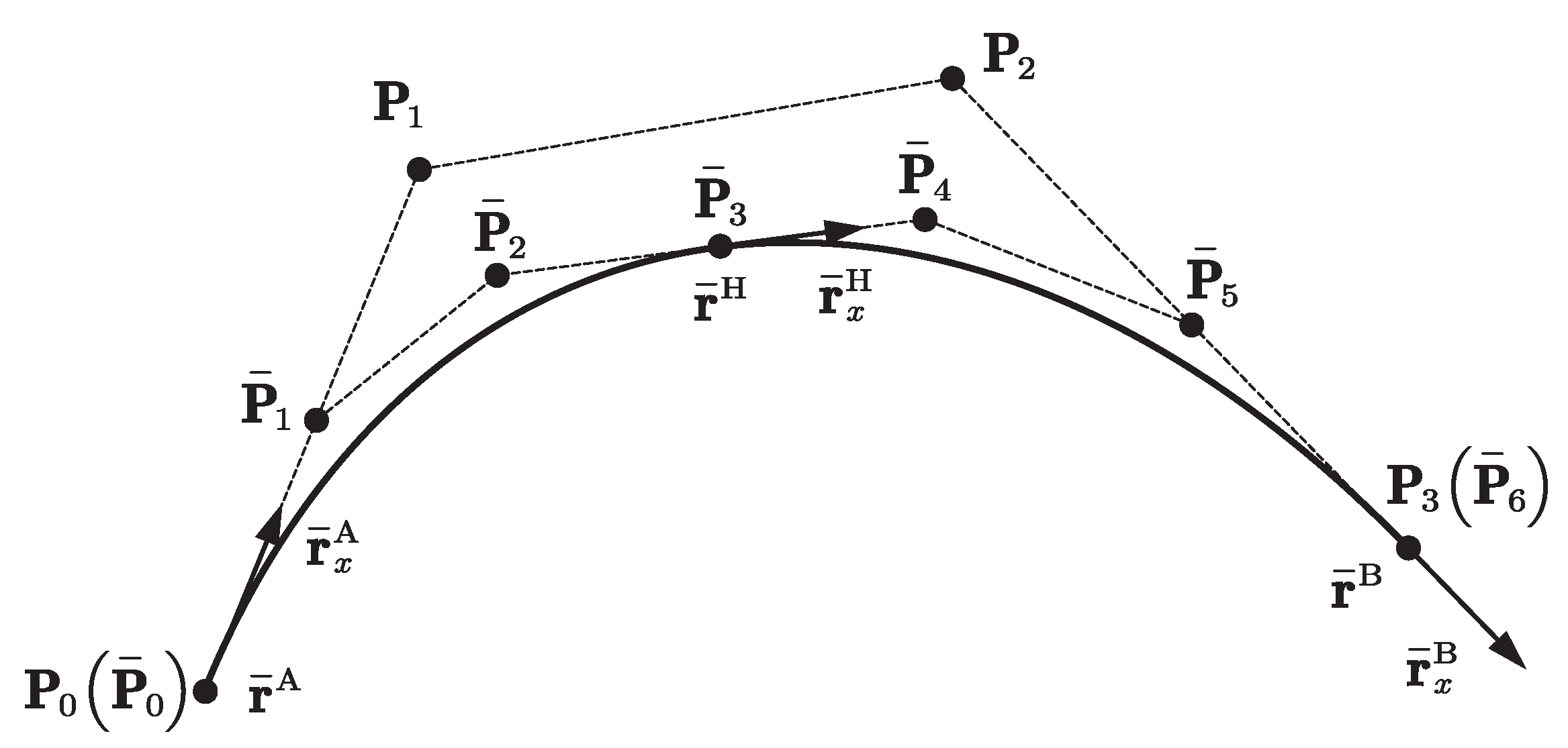
To segment the ALE-RANCF element AB shown in Figure 4, the coordinate vectors of element AB are converted to the rational Bezier control point representation by using Equation (6), and then the homogeneous coordinates and the DeCasteliau algorithm [26] are used to segment the Bezier curve. The weights and control points of the segmented Bezier curves can be calculated as:

$$\left\{\begin{array}{cc}{\overline{w}}_0=w_0,{\overline{w}}_6=w_3\hfill & {\overline{\mathbf{P}}}_0={\mathbf{P}}_0,{\overline{\mathbf{P}}}_6={\mathbf{P}}_3\hfill \\ {\overline{w}}_1={\sum }_{i=0}^1{B}_{i,1}\left(u_{\mathrm{H}}\right)w_i\hfill & {\overline{\mathbf{P}}}_1={\displaystyle \frac{1}{{\overline{w}}_1}}{\sum }_{i=0}^1{B}_{i,1}\left(u_{\mathrm{H}}\right)w_i{\mathbf{P}}_i\hfill \\ {\overline{w}}_2={\sum }_{i=0}^2{B}_{i,2}\left(u_{\mathrm{H}}\right)w_i& {\overline{\mathbf{P}}}_2={\displaystyle \frac{1}{{\overline{w}}_2}}{\sum }_{i=0}^2{B}_{i,2}\left(u_{\mathrm{H}}\right)w_i{\mathbf{P}}_i\hfill \\ {\overline{w}}_3={\sum }_{i=0}^3{B}_{i,3}\left(u_{\mathrm{H}}\right)w_i& {\overline{\mathbf{P}}}_3={\displaystyle \frac{1}{{\overline{w}}_3}}{\sum }_{i=0}^3{B}_{i,3}\left(u_{\mathrm{H}}\right)w_i{\mathbf{P}}_i\hfill \\ {\overline{w}}_4={\sum }_{i=0}^2{B}_{i,2}\left(u_{\mathrm{H}}\right)w_{i+1}& {\overline{\mathbf{P}}}_4={\displaystyle \frac{1}{{\overline{w}}_4}}{\sum }_{i=0}^2{B}_{i,2}\left(u_{\mathrm{H}}\right)w_{i+1}{\mathbf{P}}_{i+1}\hfill \\ {\overline{w}}_5={\sum }_{i=0}^1{B}_{i,1}\left(u_{\mathrm{H}}\right)w_{i+2}& {\overline{\mathbf{P}}}_5={\displaystyle \frac{1}{{\overline{w}}_5}}{\sum }_{i=0}^1{B}_{i,1}\left(u_{\mathrm{H}}\right)w_{i+2}{\mathbf{P}}_{i+2}\hfill \end{array}\right.$$

(21)

where $w_i$ and ${\overline{w}}_i$ are the weights before and after the curve is segmented, respectively. ${\mathbf{P}}_i$ and ${\overline{\mathbf{P}}}_i$ are the control points before and after the curve is segmented, respectively. $u_{\mathrm{H}}\in [0,1]$ is the parameter of the inserted node H, $B_{i,n}\left(u\right)$ are the n-degree Bernstein polynomials defined in Equation (3).

Although the weights and the control points of the Bezier curves are changed after the curve is segmented, the geometry of the curve will be exactly preserved [26], and one can demonstrate that the global parameterization, which denotes the mapping relationship between the points in the original parameter domain and the points on the Bezier curve, remains unchanged. We assume that $u\in [0,1]$ is the parameter of an arbitrary point $\mathrm{P}$ on the Bezier curve AB. If $u\in [0,u_{\mathrm{H}}]$, the point ${\mathrm{P}}^{\prime }$ that correlated to point $\mathrm{P}$ will be on the segmented curve AH, and the parameter of ${\mathrm{P}}^{\prime }$ in new parameter domain can be written as:

$$\overline{u}={\displaystyle \frac{u}{u_{\mathrm{H}}}}$$

(22)

Substituting Equations (21) and (22) into the parametric equation of the Bezier curve Equation (1), the following equation can be obtained as:

$${\mathbf{r}}^{\mathrm{AH}}\left(\overline{u}\right)={\displaystyle \frac{{\sum }_{i=0}^3{\overline{w}}_i{B}_{i,3}\left(\overline{u}\right){\overline{\mathbf{P}}}_i}{{\sum }_{i=0}^3{\overline{w}}_i{B}_{i,3}\left(\overline{u}\right)}}={\displaystyle \frac{{\sum }_{i=0}^3{w}_i{B}_{i,3}\left(u\right){\mathbf{P}}_i}{{\sum }_{i=0}^3{w}_i{B}_{i,3}\left(u\right)}}={\mathbf{r}}^{\mathrm{AB}}\left(u\right)$$

(23)

where ${\mathbf{r}}^{\mathrm{AH}}\left(\overline{u}\right)$ is the position vector of the point ${\mathrm{P}}^{\prime }$ on the segmented curve AH, and ${\mathbf{r}}^{\mathrm{AB}}\left(u\right)$ is the position vector of point $\mathrm{P}$ on the original curve AB. Similarly, if $u\in [u_{\mathrm{H}},1]$, ${\mathrm{P}}^{\prime }$ will be on the segmented curve HB, and then:

$$\overline{u}=\frac{u-u_{\mathrm{H}}}{1-u_{\mathrm{H}}}$$

(24)

The following equation can be obtained in the same way:

$${\mathbf{r}}^{\mathrm{HB}}\left(\overline{u}\right)={\mathbf{r}}^{\mathrm{AB}}\left(u\right)$$

(25)

where ${\mathbf{r}}^{\mathrm{HB}}\left(\overline{u}\right)$ is the position vector of the point ${\mathrm{P}}^{\prime }$ on the segmented curve HB. Equations (23) and (25) demonstrate that the global parameterization remains unchanged after the Bezier curve is segmented. Since the material coordinates of the ALE-RANCF element and the parameters of the Bezier curve are linearly correlated ($x=ul$), one can infer that an arbitrary material point of the ALE-RANCF element hold its position, and consequently, the exact mechanic is maintained after the ALE-RANCF element is segmented. Furthermore, one can also infer that the position coordinate and slope vector of an arbitrary node on the segmented finite element will remain unchanged as well.

The generalized coordinate vector of the segmented elements AHB can be written as:

$${\mathbf{q}}^{\mathrm{AHB}}={\left[\begin{array}{ccccccccc}{\left({\mathbf{r}}^{\mathrm{A}}\right)}^{\mathrm{T}}& {\left({\mathbf{r}}_x^{\mathrm{A}}\right)}^{\mathrm{T}}& x_{\mathrm{A}}& {\left({\mathbf{r}}^{\mathrm{H}}\right)}^{\mathrm{T}}& {\left({\mathbf{r}}_x^{\mathrm{H}}\right)}^{\mathrm{T}}& x_{\mathrm{H}}& {\left({\mathbf{r}}^{\mathrm{B}}\right)}^{\mathrm{T}}& {\left({\mathbf{r}}_x^{\mathrm{B}}\right)}^{\mathrm{T}}& x_{\mathrm{B}}\end{array}\right]}^{\mathrm{T}}$$

(26)

where

$$\left\{\begin{array}{c}\begin{array}{c}{\mathbf{r}}^{\mathrm{A}}={\overline{\mathbf{r}}}^{\mathrm{A}}={\mathbf{P}}_0,{\mathbf{r}}^{\mathrm{B}}={\overline{\mathbf{r}}}^{\mathrm{B}}={\mathbf{P}}_3,{\mathbf{r}}^{\mathrm{H}}={\overline{\mathbf{r}}}^{\mathrm{H}}={\overline{\mathbf{P}}}_3\hfill \end{array}\\ {\mathbf{r}}_x^{\mathrm{A}}={\displaystyle \frac{3w_1}{l_{\mathrm{AB}}{w}_0}}({\mathbf{P}}_1-{\mathbf{P}}_0)={\displaystyle \frac{3{\overline{w}}_1}{l_{\mathrm{AH}}{\overline{w}}_0}}({\overline{\mathbf{P}}}_1-{\overline{\mathbf{P}}}_0)={\overline{\mathbf{r}}}_x^{\mathrm{A}}\\ {\mathbf{r}}_x^{\mathrm{B}}={\displaystyle \frac{3w_2}{l_{\mathrm{AB}}{w}_3}}({\mathbf{P}}_3-{\mathbf{P}}_2)={\displaystyle \frac{3{\overline{w}}_5}{l_{\mathrm{BH}}{\overline{w}}_6}}({\overline{\mathbf{P}}}_6-{\overline{\mathbf{P}}}_5)={\overline{\mathbf{r}}}_x^{\mathrm{B}}\\ {\mathbf{r}}_x^{\mathrm{H}}={\overline{\mathbf{r}}}_x^{\mathrm{H}\left(1\right)}={\displaystyle \frac{3{\overline{w}}_2}{l_{\mathrm{AH}}{\overline{w}}_3}}({\overline{\mathbf{P}}}_3-{\overline{\mathbf{P}}}_2)={\displaystyle \frac{3{\overline{w}}_4}{l_{\mathrm{BH}}{\overline{w}}_3}}({\overline{\mathbf{P}}}_4-{\overline{\mathbf{P}}}_3)={\overline{\mathbf{r}}}_x^{\mathrm{H}\left(2\right)}\end{array}\right.$$

(27)

In these equations, ${\mathbf{r}}^{\mathrm{N}}$ and ${\overline{\mathbf{r}}}^{\mathrm{N}}$ are the nodal position coordinates of node N before and after the element is segmented, respectively. ${\mathbf{r}}_x^{\mathrm{N}}$ and ${\overline{\mathbf{r}}}_x^{\mathrm{N}}$ are the slope vectors of node N before and after the element is segmented, respectively. ${\overline{\mathbf{r}}}_x^{\mathrm{H}\left(1\right)}$ and ${\overline{\mathbf{r}}}_x^{\mathrm{H}\left(2\right)}$ are the slope vectors of the segmented elements on left and right side of the inserted node H, respectively. $l_{\mathrm{AB}}$ is the reference length of the original element AB. $l_{\mathrm{AH}}$ and $l_{\mathrm{HB}}$ are the reference lengths of the segmented elements AH and HB, respectively. The relationships between these reference lengths can be written as:

$$\left\{\begin{array}{c}{l}_{\mathrm{AB}}=x_{\mathrm{B}}-x_{\mathrm{A}}\hfill \\ l_{\mathrm{AH}}=x_{\mathrm{H}}-x_{\mathrm{A}}=u_{\mathrm{H}}{l}_{\mathrm{AB}}\hfill \\ l_{\mathrm{HB}}=x_{\mathrm{B}}-x_{\mathrm{H}}=\left(1-u_{\mathrm{H}}\right)l_{\mathrm{AB}}\hfill \end{array}\right.$$

(28)

where $x_{\mathrm{N}}$ is the material coordinate of the node N. The shape functions of the segmented element can be obtained by substituting the expressions of weights (Equation (21)) and element lengths (Equation (28)) into the shape function expression (Equation (9)).

4.2. Element Merging

Element AH and HB in Figure 5 are the ALE-RANCF elements to be merged, and element AB is the merged element. To ensure the continuity of the boundary node A and B, their nodal coordinate vectors will be maintained; therefore, the generalized coordinate vector of the merged element AB can be written as:

$${\mathbf{q}}^{\mathrm{AB}}={\left[\begin{array}{cccccc}{\left({\mathbf{r}}^{\mathrm{A}}\right)}^{\mathrm{T}}& {\left({\mathbf{r}}_x^{\mathrm{A}}\right)}^{\mathrm{T}}& x_{\mathrm{A}}& {\left({\mathbf{r}}^{\mathrm{B}}\right)}^{\mathrm{T}}& {\left({\mathbf{r}}_x^{\mathrm{B}}\right)}^{\mathrm{T}}& x_{\mathrm{B}}\end{array}\right]}^{\mathrm{T}}$$

(29)

and the reference length of the merged element is:

$$l_{\mathrm{AB}}=x_{\mathrm{B}}-x_{\mathrm{A}}=l_{\mathrm{AH}}+l_{\mathrm{HB}}$$

(30)

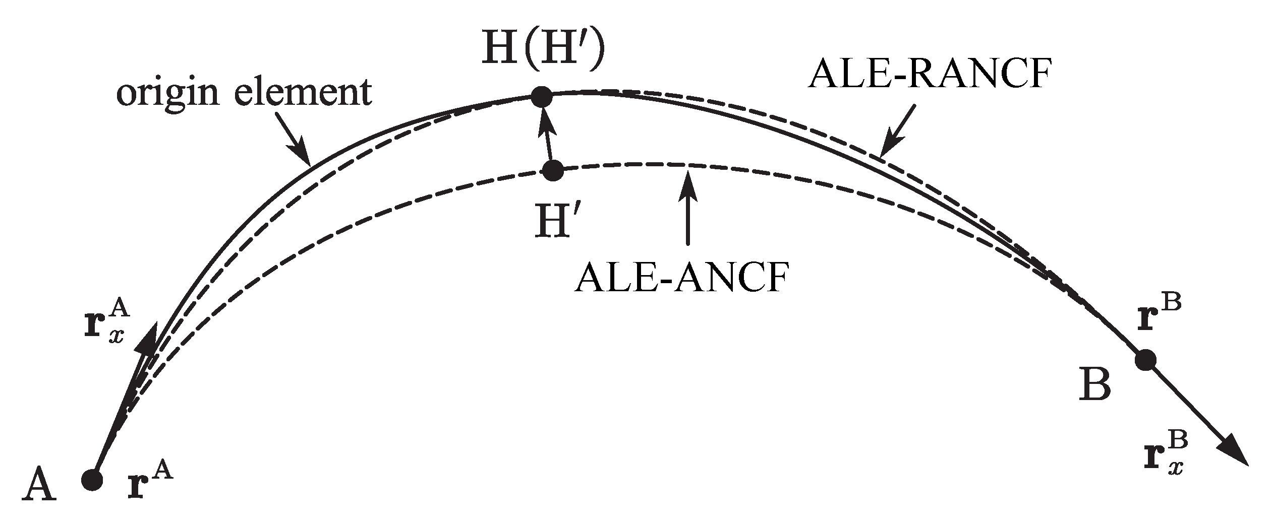
To calculate the shape functions of the merged element, the weights need to be determined. As mentioned before, due to the reduction in the degree of freedom of the system, the element alteration will be unavoidable after the elements are merged. However, the alteration could be reduced by adjusting the weights of the merged ALE-RANCF elements. An effective method to determine the weights of the merged element can be established by simply supposing the deleted node H on the original element coincides with the node ${\mathrm{H}}^{\prime }$ on the merged element. The parameter of the node ${\mathrm{H}}^{\prime }$ is defined as:

$${\overline{u}}_{\mathrm{H}}=\frac{l_{\mathrm{AH}}}{l_{\mathrm{AB}}}$$

(31)

and the following equations can be obtained as:

$${\overline{\mathbf{r}}}^{\mathrm{H}}=\overline{\mathbf{S}}\left({\overline{u}}_{\mathrm{H}}\right){\overline{\mathbf{e}}}^{\mathrm{AB}}={\mathbf{r}}^{\mathrm{H}}$$

(32)

where ${\mathbf{r}}^{\mathrm{H}}$ is the position vector of the deleted node H, ${\overline{\mathbf{r}}}^{\mathrm{H}}$ is the position vector of the node ${\mathrm{H}}^{\prime }$ correlated to H on the merged element, $\overline{\mathbf{S}}$ and ${\overline{\mathbf{e}}}^{\mathrm{AB}}$ are the shape function matrix and the generalized coordinate vector of the merged element.

Since all the weights of the ALE-RANCF elements are positive, without any loss of accuracy, one can divide the numerator and denominator of the shape functions (see Equation (9)) by $w_3$ at the same time, and the new expression of the shape functions can be written as:

$$\begin{array}{c}\left[\begin{array}{c}{s}_1\left(u\right)\\ s_2\left(u\right)\\ s_3\left(u\right)\\ s_4\left(u\right)\end{array}\right]={\displaystyle \frac{1}{K\left(u\right)}}\left[\begin{array}{c}3k_{1}u{(1-u)}^2+k_0{(1-u)}^3\\ l{k}_{0}u{(1-u)}^2\\ u^3+3k_2{u}^2(1-u)\\ -l{u}^2(1-u)\end{array}\right]\\ K\left(u\right)=u^3+3k_2{u}^2(1-u)+3k_{1}u{(1-u)}^2+k_0{(1-u)}^3>0\end{array}$$

(33)

where $k_i=w_i/w_3,i=0,1,2$. By substituting Equation (33) into Equation (32), the following linear equations with $k_i$ as unknowns can be obtained as:

$$\mathbf{f}\left(\mathbf{k}\right)={\overline{\mathbf{r}}}^{\mathrm{H}}\left(\mathbf{k}\right)-{\mathbf{r}}^{\mathrm{H}}=\mathbf{0}$$

(34)

where $\mathbf{k}={\left[\begin{array}{ccc}{k}_0& k_1& k_2\end{array}\right]}^{\mathrm{T}}$. In the two-dimensional plane case, there will be two equations and three unknowns in Equation (34); therefore, the equations theoretically have an infinite number of solutions. To optimize the parameterization of the merged element and improve the uniformity of point distribution on the element, an additional optimization target can be imposed on the solutions by minimizing the norm of vector $\mathbf{x}$ that is defined as:

$$\mathbf{x}=\mathbf{k}-\mathbf{i}$$

(35)

where $\mathbf{i}={\left[\begin{array}{ccc}1& 1& 1\end{array}\right]}^{\mathrm{T}}$. By substituting Equation (35) into Equation (34), the following linear equations with $\mathbf{x}$ as unknowns can be obtained as:

$$\mathbf{f}\left(\mathbf{k}\right)=\mathbf{f}\left(\mathbf{x}+\mathbf{i}\right)=\mathbf{Ax}-\mathbf{B}=\mathbf{0}$$

(36)

According to matrix theory, Equation (36) has a unique minimum norm least squares solution:

$$\mathbf{x}={\mathbf{A}}^{+}\mathbf{B}$$

(37)

where matrix ${\mathbf{A}}^{+}$ is the Moore–Penrose generalized inverse matrix of matrix $\mathbf{A}$. The vector $\mathbf{k}$ can be obtained by solving Equation (35). In rare cases, some of the solutions may be nonpositive, which is usually due to the large deformation of the elements to be merged, and then vector $\mathbf{k}$ will be equal to vector $\mathbf{i}$. Finally, the vector $\mathbf{k}$ can be obtained as:

$$\mathbf{k}=\left\{\begin{array}{cc}\mathbf{x}+\mathbf{i}\hfill & \mathrm{all}{x}_i+1>0\hfill \\ \mathbf{i}\hfill & \mathrm{others}\hfill \end{array}\right.$$

(38)

where $x_i,i=0,1,2$ are the elements of vector $\mathbf{x}$. In the three-dimensional space case, there will be three equations and three unknowns in Equation (34). If the equations are consistent, it can be directly solved; otherwise, one can solve its minimum norm least squares solution using Equations (35)–(38). By substituting Equations (30) and (38) into Equation (33), one can finally calculate the shape functions of the merged ALE-RANCF element.

5. Sliding Joint Model

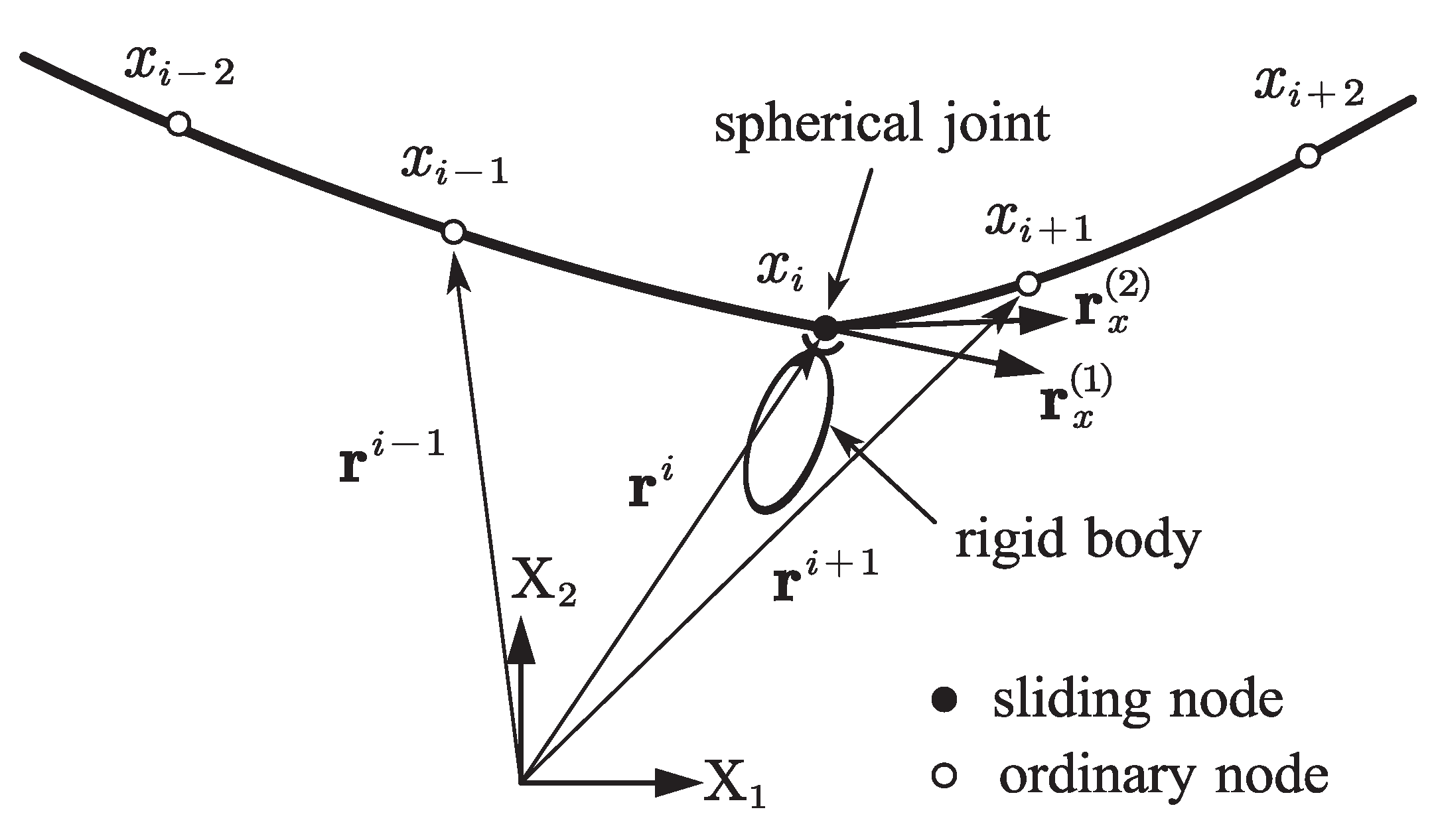
The sliding joint model is developed using the ALE-RANCF elements as shown in Figure 6. The sliding node is coupled with a moving node on the axis of the beam, which is realized by changing the length of the two adjacent elements of the sliding joint in a conjugate way. Slope vectors on two sides of the sliding joint are adopted as the generalized coordinates to capture the discontinuity of the slopes. For efficiency, only elements adjacent to the sliding joint are the variable-length ALE-RANCF elements, and other elements are the fixed-length RANCF elements. The generalized coordinate vector of the beam can be written as:

$$\begin{array}{c}\hfill {\mathbf{q}}_c=[\begin{array}{ccccccccc}{\left({\mathbf{r}}^1\right)}^{\mathrm{T}}& {\left({\mathbf{r}}_x^1\right)}^{\mathrm{T}}& \cdots & {\left({\mathbf{r}}^{i-1}\right)}^{\mathrm{T}}& {\left({\mathbf{r}}_x^{i-1}\right)}^{\mathrm{T}}& {\left({\mathbf{r}}^i\right)}^{\mathrm{T}}& {\left({\mathbf{r}}_x^{i\left(1\right)}\right)}^{\mathrm{T}}& {\left({\mathbf{r}}_x^{i\left(2\right)}\right)}^{\mathrm{T}}& x_i\end{array}\\ \hfill \begin{array}{ccccc}{\left({\mathbf{r}}^{i+1}\right)}^{\mathrm{T}}& {\left({\mathbf{r}}_x^{i+1}\right)}^{\mathrm{T}}& \cdots & {\left({\mathbf{r}}^N\right)}^{\mathrm{T}}& {\left({\mathbf{r}}_x^N\right)}^{\mathrm{T}}\end{array}]\end{array}$$

(39)

where i is the number of the sliding node, N is the total number of the beam nodes, ${\mathbf{r}}_x^{i\left(1\right)}$ and ${\mathbf{r}}_x^{i\left(2\right)}$ are the slope vectors on the left and right side of the sliding joint, respectively. When the slopes on two sides of the sliding node are continuous or discontinuous, the constraints on the slope vectors can be expressed as:

$${\mathbf{C}}^s\left({\mathbf{r}}_x^{i\left(1\right)},{\mathbf{r}}_x^{i\left(2\right)}\right)=\left\{\begin{array}{c}\begin{array}{cc}{\mathbf{r}}_x^{i\left(1\right)}-{\mathbf{r}}_x^{i\left(2\right)}=\mathbf{0}\hfill & \mathrm{continuous}\mathrm{slopes}\hfill \end{array}\\ \left|{\mathbf{r}}_x^{i\left(1\right)}\right|-\left|{\mathbf{r}}_x^{i\left(2\right)}\right|=0\hspace{1em}\mathrm{discontinuous}\mathrm{slopes}\end{array}\right.$$

(40)

Assembling governing equations of all the beam elements and the rigid body, and combining all the constraint equations, one can obtain the dynamic equations with constraint equations in the following standard form of multibody systems: [31]

$$\left\{\begin{array}{c}\begin{array}{c}\mathbf{M}\ddot{\mathbf{q}}+{\mathbf{C}}_{\mathbf{q}}^{\mathrm{T}}\lambda -\mathbf{Q}\left(\dot{\mathbf{q}},\mathbf{q},t\right)=\mathbf{0}\hfill \end{array}\\ \mathbf{C}\left(\mathbf{q},t\right)=\mathbf{0}\end{array}\right.$$

(41)

In this equation, $\mathbf{M}$ the system mass matrix, $\mathbf{q}$ is the system generalized coordinate vector, $\mathbf{Q}\left(\dot{\mathbf{q}},\mathbf{q},t\right)$ is the system generalized force vector, $\mathbf{C}\left(\mathbf{q},t\right)$ is the constraint conditions and ${\mathbf{C}}_{\mathbf{q}}=\partial \mathbf{C}/\partial \mathbf{q}$ is the Jacobian matrix of the constraints, and $\lambda$ is the vector of Lagrange multipliers. Equation (41) is a differential algebraic equation, and it can be solved numerically by using the generalized-$\alpha$ method [32].

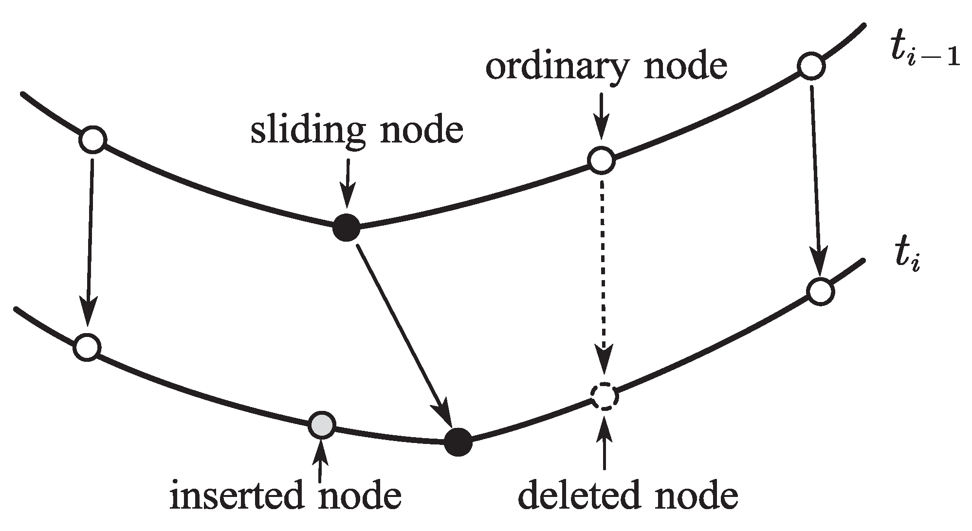
The illustration of the element length-control scheme of the sliding joint model is represented in Figure 7. Without loss of generality, assuming that the reference length of all elements in the initial configuration is $L_{std}$. In a practical simulation, if the reference length of the element on one side of the sliding node exceeds the given threshold length ($1.5L_{std}$), a new node could be inserted into the element to divide it into two new elements, and the reference length of the new element away from the sliding node should be $L_{std}$. The adjacent node on the other side of the sliding joint should be deleted at the same time. Reference length of all elements is controlled in the range of $0.5L_{std}$ to $1.5L_{std}$, and therefore, too long or too short elements are avoided. The node number of the beam and the dimension of the generalized coordinate vector of the sliding joint model will always remain constant as well.

6. Numerical Examples

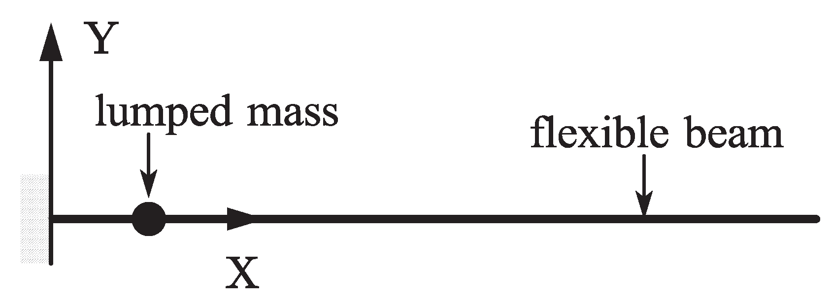
6.1. A Falling Beam with a Sliding Lumped Mass

A lumped mass point slides along a falling beam without friction under gravity is shown in Figure 8. The left end of the beam is fixed supported and the right end is free. The reference length of the beam is set to 1 m, the cross-section radius is set to 0.01 m, the density is set to 7200 $\mathrm{kg}/{\mathrm{m}}^3$, Young’s modulus is set to 20 MPa, the damping effect is neglected. The lumped mass is 0.8 kg, its initial position is 0.1 m from the left end of the beam and its initial speed is 0. A sliding joint is introduced to simulate the relationship between the lumped mass and the flexible beam. Two dynamic models are developed based on the ALE-RANCF and ALE-ANCF. A similar model based on ALE-ANCF was presented and the results were analyzed in paper [10]. The results of the two models are analyzed and compared as follows.

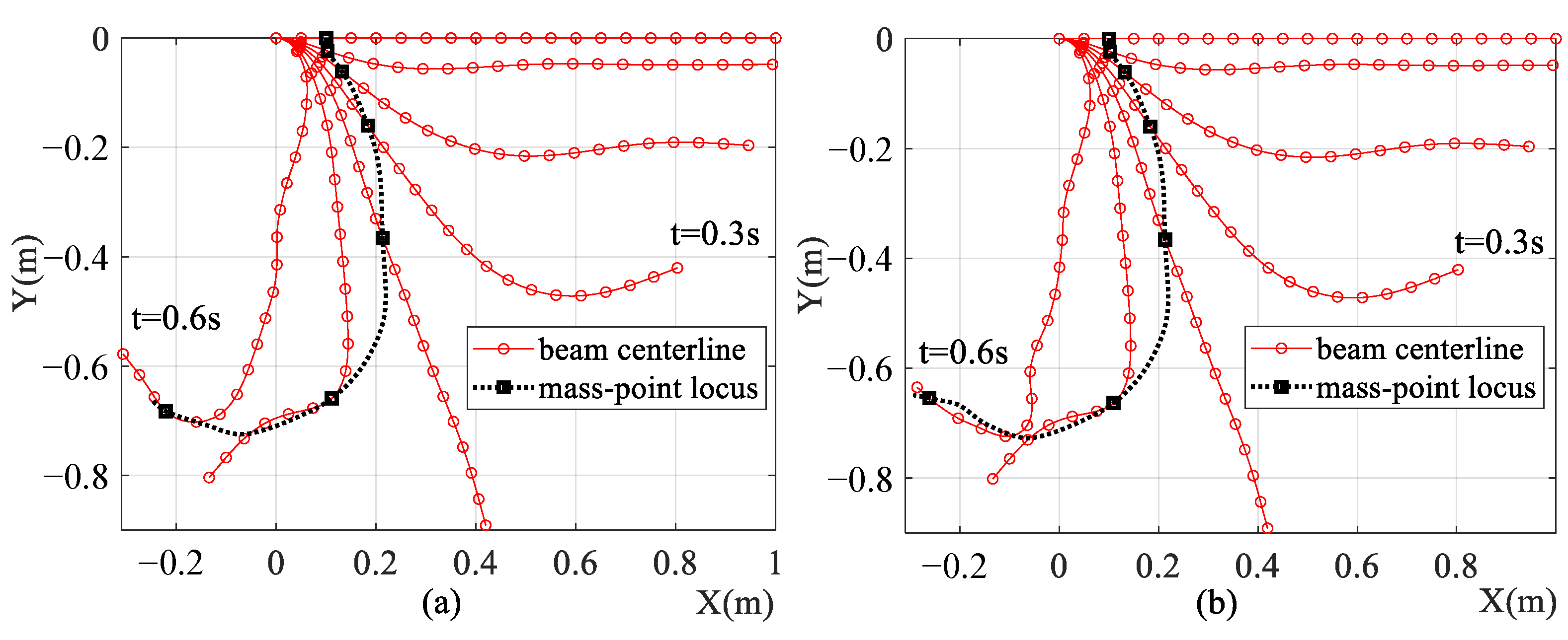
The configurations of the falling beam and the lumped mass are shown in Figure 9. The lumped mass is separated from the beam in 0.6 s to 0.7 s. The beam is divided into 20 elements, and one can see from Figure 9 that the configurations between the ALE-RANCF model and the ALE-ANCF model are very similar.

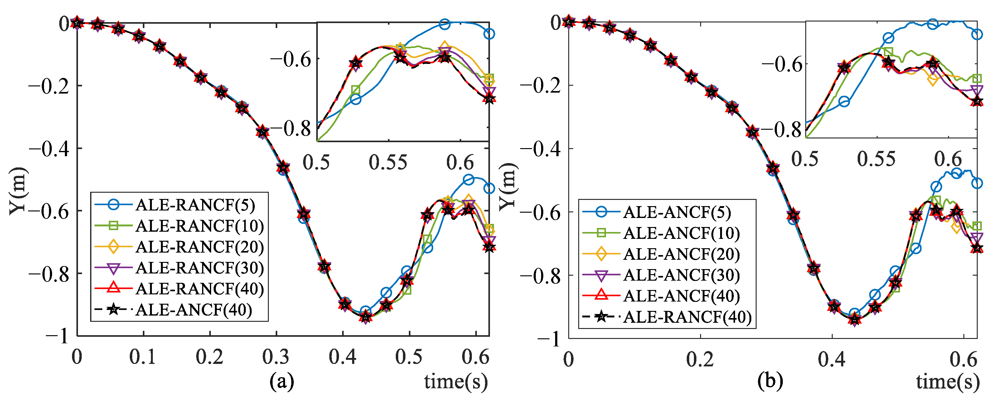
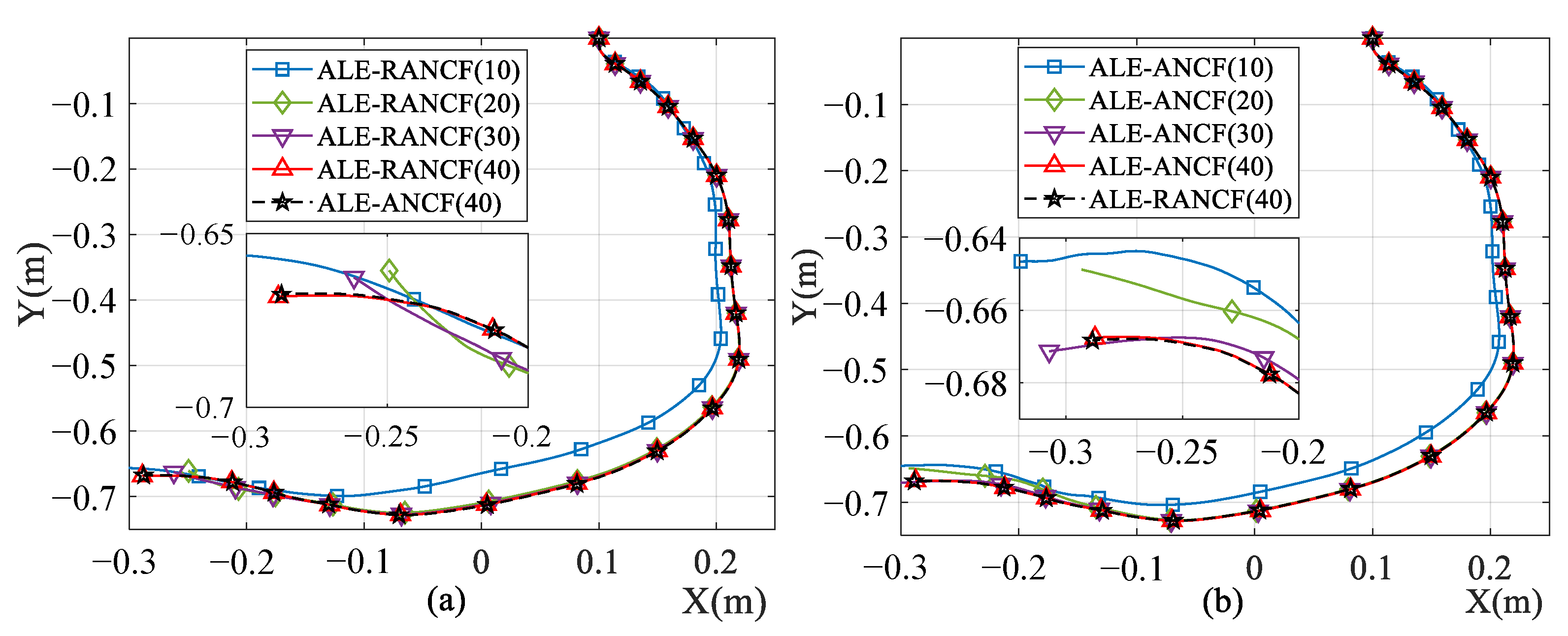
Figure 10 shows the Y-axis displacement of the right end node of the beam. Figure 11 shows the trajectories of the sliding nodes. The numbers in the legends of figures denote the numbers of the beam elements. One can see that as the element number increases, the simulation results of both models tend to converge. When the element number increases to 40, the results of the ALE-RANCF model and ALE-ANCF model are almost identical.

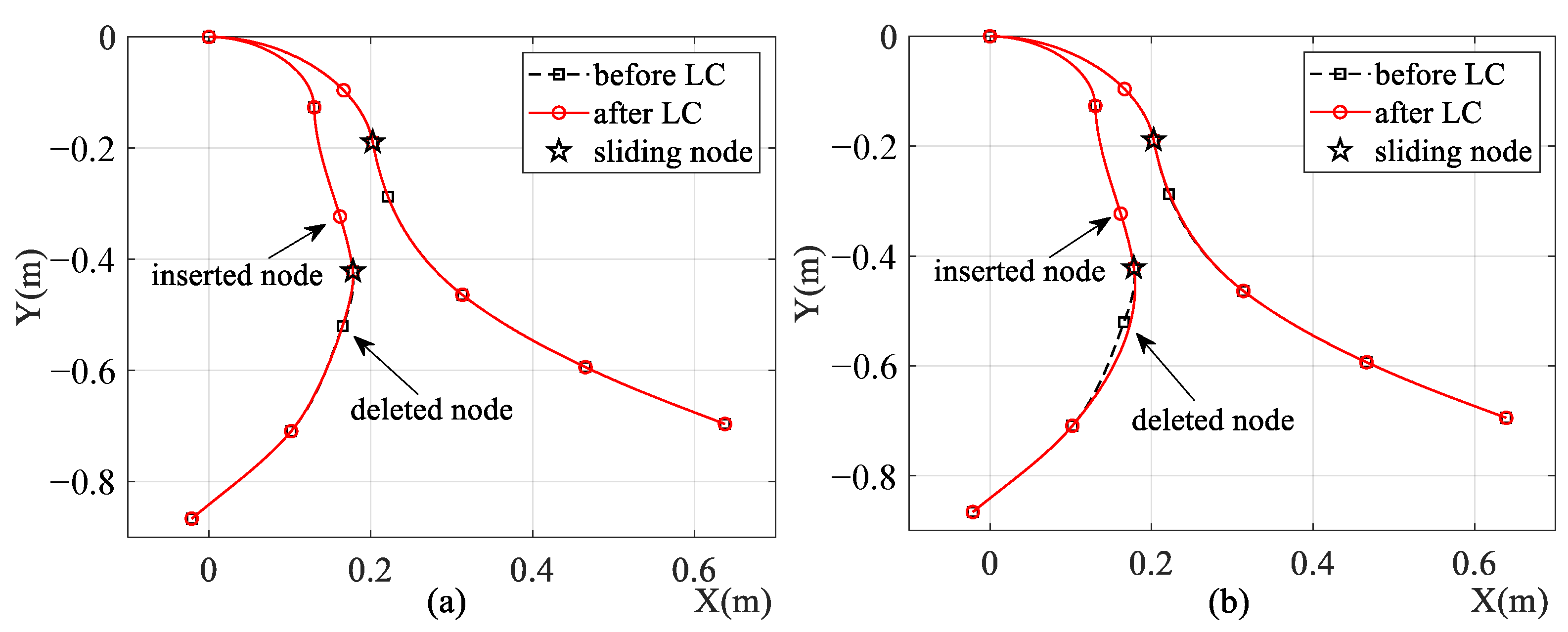
Figure 12 shows the configurations of both models before and after element length control. The beams of both models are divided into five elements, and element length control is carried out twice. One can see from Figure 12 that exact element shapes are maintained after elements are segmented in both models, while element shape alterations in the ALE-RANCF model are smaller than the element shape alterations in the ALE-ANCF model.

Table 1. Statistical results of simulation time of ALE-RANCF and the ALE-ANCF models. LC is short for length-control.

Number of Elements	LC Times	ALE-RANCF		ALE-ANCF
		Motion Time(s)	LC Time(s)	Motion Time(s)	LC Time(s)
5	3	59.9	16.1	34.6	/
10	9	97.1	69.1	58.3	/
20	18	169.2	157.0	103.1	/
30	26	292.4	238.3	192.4	/
40	35	478.0	378.2	325.0	/

shows the statistical results of the simulation time of the two models with different number of elements. The total simulation time consists of the motion time and the length-control time. The motion time is the simulation time when the beam and the lumped mass are actually moving, and the length-control time is the simulation time of node insertion and deletion. One can see from Table 1 that the motion time of both models increases with the number of elements. Because of the complex rational shape function of the ALE-RANCF elements (Equation (9)), the motion time of the ALE-RANCF models is on average about 1.6 times that of the ALE-ANCF model. The length-control time of the ALE-RANCF model increases with the length-control times, while the length-control time of the ALE-ANCF model is too short to be correctly obtained in the simulation program. In a practical simulation, the length-control times and the number of elements may not be correlated; therefore, the influence of length-control time should be measured according to the specific simulation objects.

Table 2. Statistical results of weight sets of ALE-RANCF model.

Number of Elements	Size of Set	Maximum	Minimum	Deviation $\left(\mathit{\sigma }\right)$
5	6	1.32	0.44	0.27
10	24	1.18	0.12	0.29
20	57	1.15	0.73	0.06
30	81	1.16	0.95	0.03
40	108	1.07	0.72	0.04

presents the statistical results of the weight sets of the ALE-RANCF model with different element numbers. The weights in Table 2 refer to the parameters in Equation (33), which are transformed from original weights. The initial weight set is a null set, and new weights will be added to the set when new element weights are calculated in the element length-control process. The deviation $\sigma$ in Table 2 is defined as:

$$\sigma =\sqrt{\frac{1}{N}\sum _{i=1}^N{\left(k_i-1\right)}^2}$$

(42)

where $k_i,i\in [1,N]$ are the elements in the weight set, N is the size of the weight set. One can see that the weights of the ALE-RANCF elements tend to 1 as the element number increases, and it implies that the dynamic model based on ALE-RANCF and ALE-ANCF tend to be identical.

6.2. A Suspended Beam with a Sliding Lumped Mass

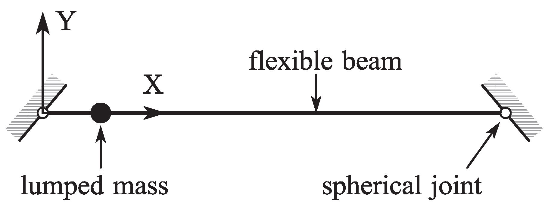
A lumped mass point slides along a suspended beam without friction under gravity as shown in Figure 13. The beam has the same properties as the beam in example 1, and both the left- and right-ends of the beam are simply supported. The lumped mass is 5 kg, its initial position is 0.1 m from the left-end of the beam, and its initial speed is 0. Two dynamic models are developed based on the ALE-RANCF and ALE-ANCF, the beams in both models are divided into three elements, and the results of the two models are analyzed and compared as follows.

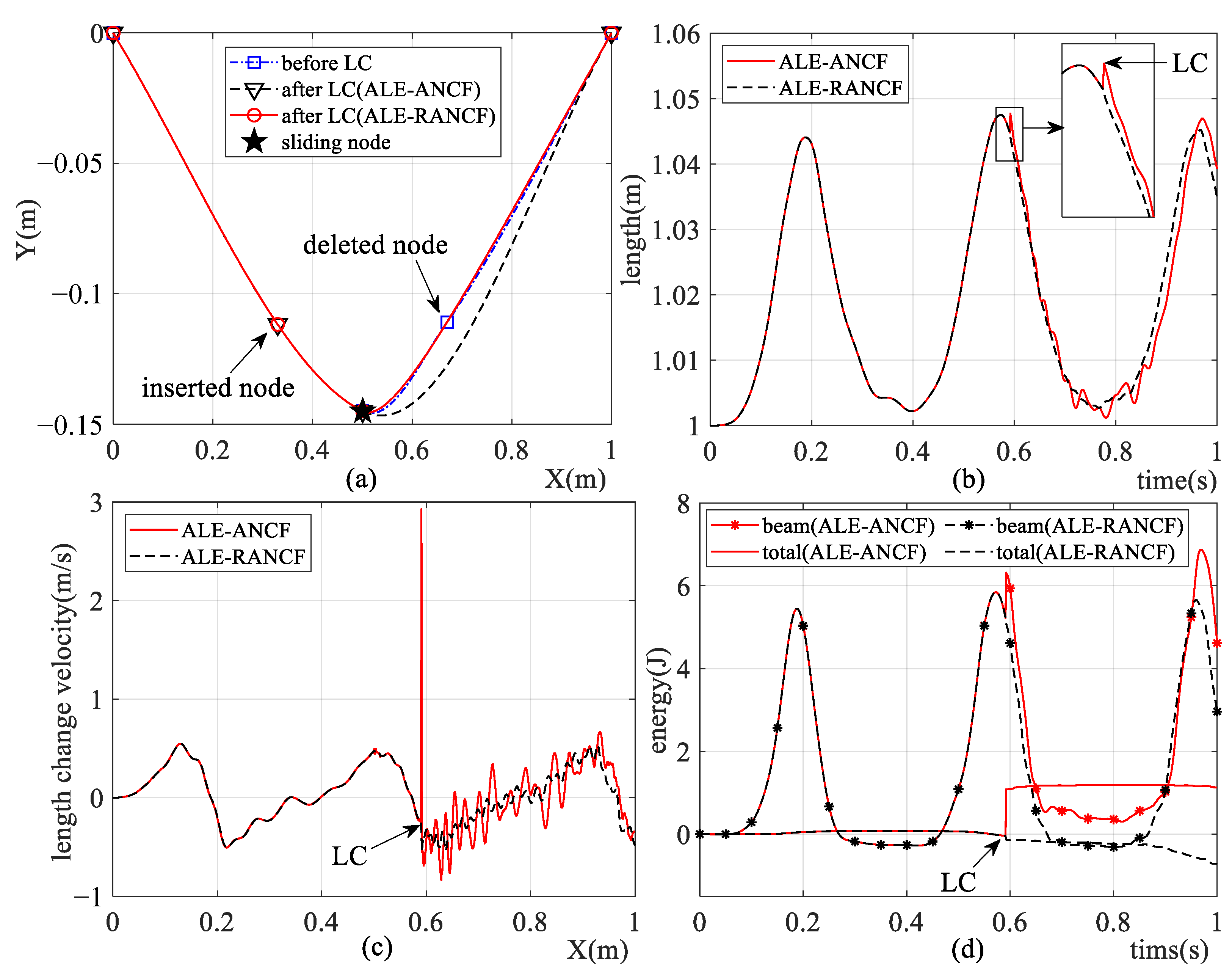
All the initial weights of the ALE-RANCF elements are equal to 1; therefore, one can consider that the ALE-RANCF and ALE-ANCF model are equivalent before the element length-control process is carried out. Figure 14 shows the simulation results of two models. One can see from Figure 14 that exact shapes are maintained after the element is divided in both models, while the shape alterations of elements, abrupt changes and vibrations of the beam length, and system energies arise after elements are merged in both models. But the geometric alterations of elements, as well as the state vibrations in the ALE-RANCF model, are smaller than they are in the ALE-ANCF model.

6.3. A Suspended Semicircular Beam with a Sliding Lumped Mass

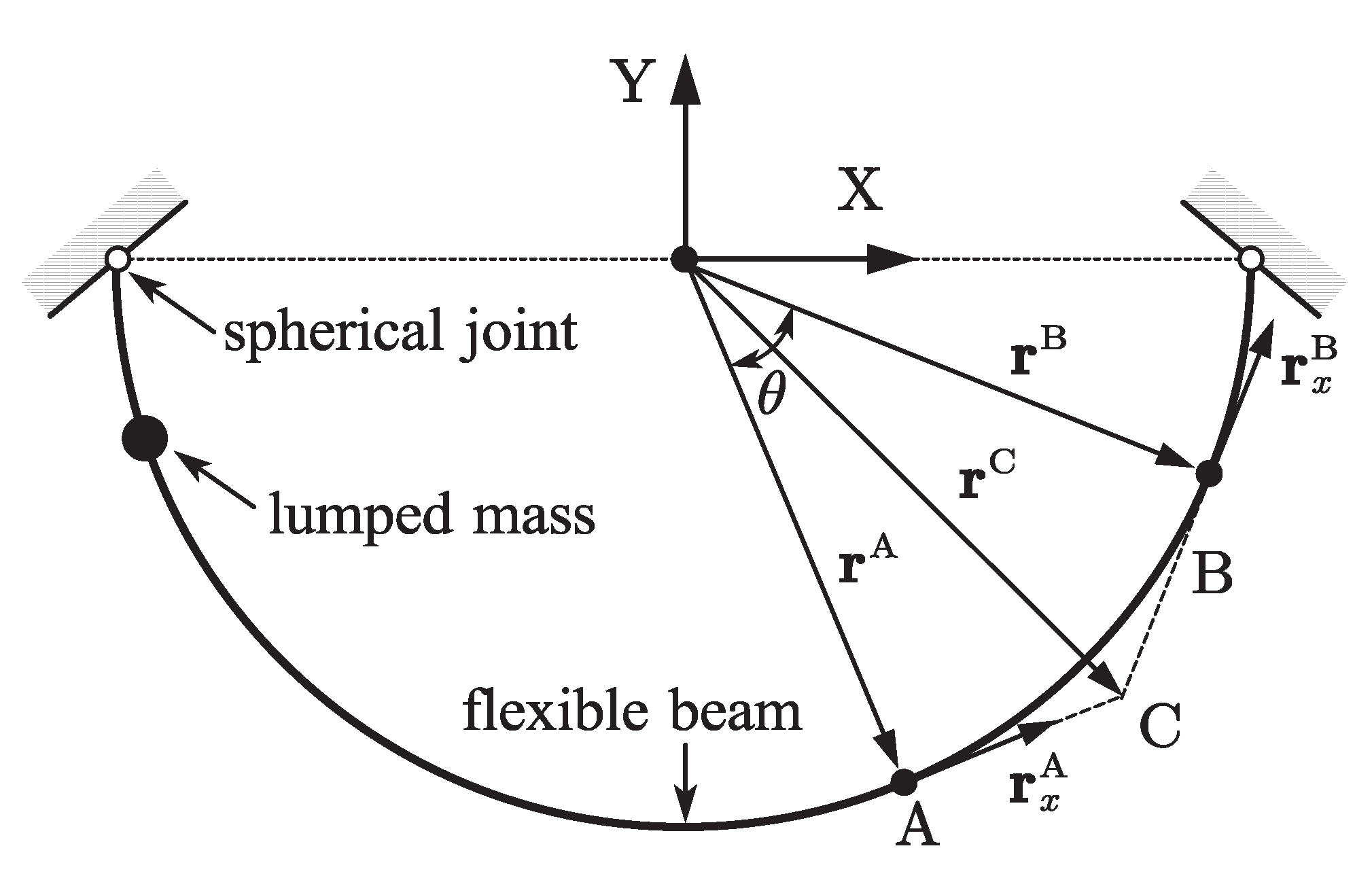
A lumped mass point slides along a suspended semicircular beam without friction under gravity as shown in Figure 15. Both the left- and right-ends of the beam is simply supported. The semicircle radius is set to 2 m, the cross-section radius of the beam is set to 0.02 m, the density is set to 7200 $\mathrm{kg}/{\mathrm{m}}^3$, Young’s modulus is set to 200 MPa, and the damping effect is neglected. The lumped mass is 0.8 kg, its initial position is set to 1/16 of the beam length from the left-end of the beam, and its initial speed is 0. A dynamic model is established using the ALE-RANCF finite elements.

The rational Bezier curve description method of the arc curve was introduced in reference [26]. Element AB shown in Figure 15 is an arbitrary circular arc ALE-RANCF element, and the tangent lines at the end node A and B intersect at point C. The weights and nodal coordinate gradients of element AB can be formulated as:

$$\left\{\begin{array}{c}{w}_0=w_3=1\hfill \\ w_1=w_2={\displaystyle \frac{1+2cos(\theta /2)}{3}}\hfill \\ {\mathbf{r}}_x^{\mathrm{A}}={\displaystyle \frac{2}{\theta R}}cos\left(\theta /2\right)\left({\mathbf{r}}^{\mathrm{C}}-{\mathbf{r}}^{\mathrm{A}}\right)\hfill \\ {\mathbf{r}}_x^{\mathrm{B}}={\displaystyle \frac{2}{\theta R}}cos\left(\theta /2\right)\left({\mathbf{r}}^{\mathrm{B}}-{\mathbf{r}}^{\mathrm{C}}\right)\hfill \end{array}\right.$$

(43)

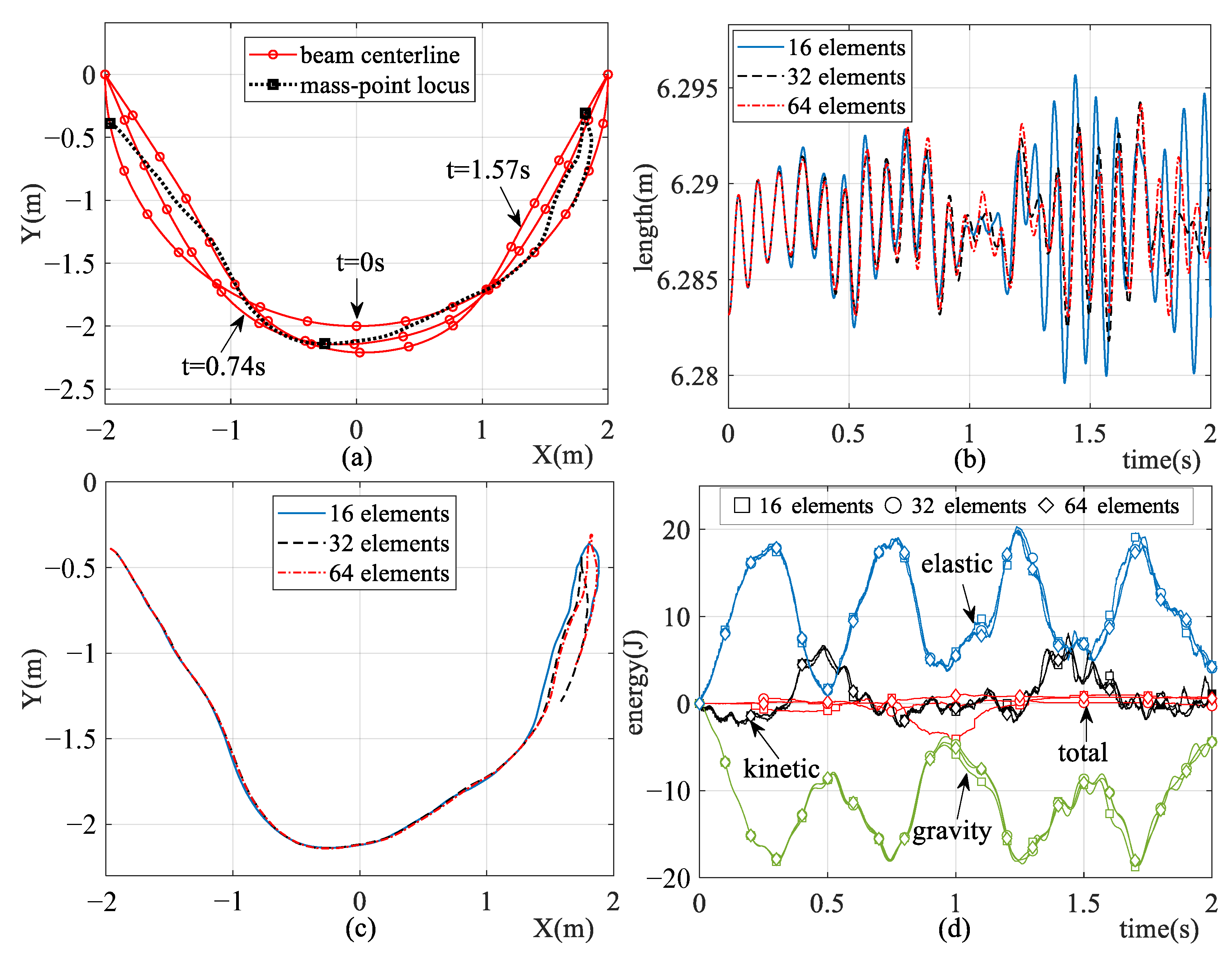
where R, $\theta <\pi$ are the radius and central angle of arc AB. The simulation results are shown in Figure 16. One can see that the shape of the semicircular beam is exactly described by using the ALE-RANCF finite elements at the initial time, and as the number of the beam elements increases, the simulation results tend to converge.

7. Conclusions

The ALE-RANCF finite element was established by combining the desirable features of the ALE-ANCF and the RANCF finite elements. The variable-length ALE-RANCF finite elements could be used to construct the dynamic model for sliding joint efficiently and effectively, and it could also capture the exact geometry of rational cubic Bezier curves, such as conic and circular curves.

The length-control scheme for ALE-RANCF finite elements, including the element segmentation and merging scheme, is proposed. It is theoretically demonstrated that the element segmentation scheme maintains exact geometry and mechanic after elements are divided. Compared with that of the ALE-ANCF elements, there are smaller geometric deviations and state vibrations after the ALE-RANCF elements are merged.

The feasibility and advantages of the ALE-RANCF finite elements are demonstrated with numerical examples.

References

- Sugiyama, H.; Escalona, J.L.; Shabana, A.A. Formulation of three-dimensional joint constraints using the absolute nodal coordinates. Nonlinear Dyn. 2003, 31, 167–195. [Google Scholar] [CrossRef]
- Muñoz, J.J.; Jelenić, G. Sliding joints in 3D beams: Conserving algorithms using the master-slave approach. Multibody Syst. Dyn. 2006, 16, 237–261. [Google Scholar] [CrossRef] [Green Version]
- Mizuno, Y.; Sugiyama, H. Sliding and nonsliding joint constraints of B-spline plate elements for integration with flexible multibody dynamics simulation. J. Comput. Nonlinear Dyn. 2014, 9, 011001. [Google Scholar] [CrossRef]
- Lee, S.H.; Park, T.W.; Seo, J.H.; Yoon, J.W.; Jun, K.J. The development of a sliding joint for very flexible multibody dynamics using absolute nodal coordinate formulation. Multibody Syst. Dyn. 2008, 20, 223–237. [Google Scholar] [CrossRef]
- Gu, Y.; Lan, P.; Cui, Y.; Li, K.; Yu, Z. Dynamic interaction between the transmission wire and cross-frame. Mech. Mach. Theory 2021, 155, 104068. [Google Scholar] [CrossRef]
- Kulkarni, S.; Pappalardo, C.M.; Shabana, A.A. Pantograph/catenary contact formulations. ASME J. Vib. Acoust. 2016, 139, 011010. [Google Scholar] [CrossRef]
- Tang, J.; Ren, G.; Zhu, W.; Ren, H. Dynamics of variable-length tethers with application to tethered satellite deployment. Commun. Nonlinear Sci. Numer. Simul. 2011, 16, 3411–3424. [Google Scholar] [CrossRef]
- Luo, C.; Sun, J.; Wen, H.; Jin, D. Dynamics of a tethered satellite formation for space exploration modeled via ANCF. Acta Astronaut. 2020, 177, 882–890. [Google Scholar] [CrossRef]
- Zhang, H.; Guo, J.Q.; Liu, J.P.; Ren, G.X. An efficient multibody dynamic model of arresting cable systems based on ALE formulation. Mech. Mach. Theory 2020, 151, 103892. [Google Scholar] [CrossRef]
- Hong, D.; Ren, G. A modeling of sliding joint on one-dimensional flexible medium. Multibody Syst. Dyn. 2011, 26, 91–106. [Google Scholar] [CrossRef]
- Hong, D.; Tang, J.; Ren, G. Dynamic modeling of mass-flowing linear medium with large amplitude displacement and rotation. J. Fluids Struct. 2011, 27, 1137–1148. [Google Scholar] [CrossRef]
- Gerstmayr, J.; Sugiyama, H.; Mikkola, A. Review on the absolute nodal coordinate formulation for large deformation analysis of multibody systems. J. Comput. Nonlinear Dyn. 2013, 8, 031016. [Google Scholar] [CrossRef]
- Shabana, A.A. Definition of ANCF finite elements. J. Comput. Nonlinear Dyn. 2015, 10, 054506. [Google Scholar] [CrossRef]
- Ren, H.; Fan, W.; Zhu, W.D. An accurate and robust geometrically exact curved beam formulation for multibody dynamic analysis. ASME J. Vib. Acoust. 2017, 140, 011012. [Google Scholar] [CrossRef]
- Otsuka, K.; Wang, Y.; Fujita, K.; Nagai, H.; Makihara, K. Multifidelity modeling of deployable wings: Multibody dynamic simulation and wind tunnel experiment. AIAA J. 2019, 57, 4300–4311. [Google Scholar] [CrossRef]
- Kim, E.; Kim, H.; Cho, M. Model order reduction of multibody system dynamics based on stiffness evaluation in the absolute nodal coordinate formulation. Nonlinear Dyn. 2017, 87, 1901–1915. [Google Scholar] [CrossRef]
- Qi, Z.; Wang, J.; Wang, G. An efficient model for dynamic analysis and simulation of cable-pulley systems with time-varying cable lengths. Mech. Mach. Theory 2017, 116, 383–403. [Google Scholar] [CrossRef]
- Peng, Y.; Wei, Y.; Zhou, M. Efficient modeling of cable-pulley system with friction based on arbitrary-Lagrangian-Eulerian approach. Appl. Math. Mech. 2017, 38, 1785–1802. [Google Scholar] [CrossRef]
- Wang, J.; Qi, Z.; Wang, G. Hybrid modeling for dynamic analysis of cable-pulley systems with time-varying length cable and its application. J. Sound Vib. 2017, 406, 277–294. [Google Scholar] [CrossRef]
- Sanborn, G.G.; Shabana, A.A. A rational finite element method based on the absolute nodal coordinate formulation. Nonlinear Dyn. 2009, 58, 565. [Google Scholar] [CrossRef]
- Lan, P.; Shabana, A.A. Rational finite elements and flexible body dynamics. J. Vib. Acoust. 2010, 132, 041007. [Google Scholar] [CrossRef]
- Yamashita, H.; Sugiyama, H. Numerical convergence of finite element solutions of nonrational B-spline element and absolute nodal coordinate formulation. Nonlinear Dyn. 2012, 67, 177–189. [Google Scholar] [CrossRef]
- Mikkola, A.; Shabana, A.A.; Sanchez-Rebollo, C.; Jimenez-Octavio, J.R. Comparison between ANCF and B-spline surfaces. Multibody Syst. Dyn. 2013, 30, 119–138. [Google Scholar] [CrossRef]
- Nada, A.A. Use of B-spline surface to model large-deformation continuum plates: Procedure and applications. Nonlinear Dyn. 2013, 72, 243–263. [Google Scholar] [CrossRef]
- Hughes, T.J.R.; Cottrell, J.A.; Bazilevs, Y. Isogeometric analysis: CAD, finite elements, NURBS, exact geometry and mesh refinement. Comput. Methods Appl. Mech. Eng. 2005, 194, 4135–4195. [Google Scholar] [CrossRef] [Green Version]
- Piegl, L.A.; Tiller, W. The NURBS Book, 2nd ed.; Springer: New York, NY, USA, 1997. [Google Scholar] [CrossRef]
- Sanborn, G.G.; Shabana, A.A. On the integration of computer aided design and analysis using the finite element absolute nodal coordinate formulation. Multibody Syst. Dyn. 2009, 22, 181–197. [Google Scholar] [CrossRef]
- Fan, W.; Zhu, W.D. An accurate singularity-free formulation of a three-dimensional curved Eule-Bernoulli beam for flexible multibody dynamic analysis. ASME J. Vib. Acoust. 2016, 138, 051001. [Google Scholar] [CrossRef]
- Gerstmayr, J.; Shabana, A.A. Analysis of thin beams and cables using the absolute nodal co-ordinate formulation. Nonlinear Dyn. 2006, 45, 109–130. [Google Scholar] [CrossRef]
- Berzeri, M.; Shabana, A. Development of simple models for the elastic forces in the absolute nodal coordinate formulation. J. Sound Vib. 2000, 235, 539–565. [Google Scholar] [CrossRef]
- Shabana, A.A. Dynamics of Multibody Systems; Cambridge University Press: Cambridge, UK, 2013. [Google Scholar] [CrossRef]
- Arnold, M.; Brüls, O. Convergence of the generalized-α scheme for constrained mechanical systems. Multibody Syst. Dyn. 2007, 18, 185–202. [Google Scholar] [CrossRef]
Figure 1.
Rational absolute nodal coordinate formulation (RANCF) beam element model.
Figure 2.
Arbitrary Lagrange–Euler absolute nodal coordinate formulation (ALE-RANCF) beam element model ( and are axes of the global coordinate system).
Figure 3.
Illustrations of (a) element segmentation and (b) element merging scheme.
Figure 4.
Segmentation of ALE-RANCF element.
Figure 5.
Merging of ALE-RANCF elements.