Multi-Sensor Data Driven with PARAFAC-IPSO-PNN for Identification of Mechanical Nonstationary Multi-Fault Mode

Abstract

Data analysis has wide applications in eliminating the irrelevant and redundant components in signals to reveal the important informational characteristics that are required. Conventional methods for multi-dimensional data analysis via the decomposition of time and frequency information that ignore the information in signal space include independent component analysis (ICA) and principal component analysis (PCA). We propose the processing of a signal according to the continuous wavelet transform and the construction of a three-dimensional matrix containing the time–frequency–space information of the signal. The dimensions of the three-dimensional matrix are reduced by parallel factor analysis, and the time characteristic matrix, frequency characteristic matrix, and spatial characteristic matrix are obtained with tensor decomposition. Through the comparative analysis of the simulation and the experiment, the time characteristic matrix and the frequency characteristic matrix can accurately characterize the normal and fault states of the mechanical equipment. On this basis, the authors established a probabilistic neural network classification model optimized by the improved particle swarm algorithm (IPSO). The parallel factor (PARAFAC) decomposition algorithm can extract features from the centrifugal pump experimental data for normal and multiple fault states, establish the mapping relationship of different fault features of the centrifugal pump in time, frequency, and space, and import the fault features into the model classification. The above measures can significantly improve the fault identification rate and accuracy for a centrifugal pump.

1. Introduction

Since the beginning of the computer era, machinery and equipment systems in the context of Industry 4.0 have become more complex and systematic. For ensuring the stability and continuity of machinery in industrial production, it is important to precisely monitor the state of machines in operation and rapidly determine the location of faults. Enterprises and researchers have paid more and more attention to the related fault diagnosis technology. Oil monitoring, accelerometer sensor monitoring, acoustic monitoring, running state degradation, and NDT flaw detection are the major fault identification technological approaches in machinery fault diagnosis. The rapid progress in computer science, measurement technology, and signal processing has promoted mechanical fault diagnosis from these methods, which include the physical models, signal processing, and the new process of using data-driven technology [1,2,3]. While traditional fault diagnosis methods cannot handle signals collected under complex conditions due to the low computing and storage capacity of computers, the current modern condition monitoring technology has been greatly improved in both theory and technology to the extent that the optimized system can realize data collection on complex equipment at multiple measurement points and throughout their whole life. The inspection system will obtain a large amount of data, machinery, and equipment fault diagnosis experience and gradually approach what is known as “big data” [4,5,6].

Centrifugal pumps are extensively used in the aerospace, oil, ocean, agriculture, chemistry, and nuclear industries, because of their energy efficiency, space savings, and stability [7,8,9]. Nowadays, this kind of equipment is mostly in service in the large-scale and complex processes of industrial production lines that are “non-stop”. Due to the interference of internal and external factors such as operating and environmental conditions, various failures such as vibration and wear often occur during operation. If minor faults are not detected in their early stages and the corresponding fault causes are not investigated, the actual heavy load and high-speed operating conditions will cause accelerated damage to the pump body and other important components, leading to the evolution and transmission of the fault [10,11,12]. In order to maintain the safe and continuous service of these pumps and conserve their industrial and economic benefits, the diagnosis and monitoring of centrifugal pump fault status cannot be ignored [13]. Current research on centrifugal pumps by scholars from various countries has focused on fault diagnosis and monitoring the health of rotor system instability, impeller cavitation, and cavitation [14]. As the core component of the pump, the impeller takes on a direct role in promoting the fluid. In actual production, the liquid component carried by the centrifugal pump usually contains solid particles such as sediment and corrosive components. These components frequently cause damage such as the cavitation, corrosion, and abrasion of the impeller in close contact with the liquid, which intensifies the vibration of the pump unit and reduces the overall hydraulic performance and reliability of the pump [15,16,17]. Therefore, the choice of centrifugal pump impeller, which is the research object of this paper, has far-reaching practical significance.

Scholars in related fields throughout the world have proposed their own unique, effective, and advanced theories and innovative methodologies in the feature extraction of fault information, sensor signal fusion with artificial intelligence for the different mechanical fault types and characteristics, and have achieved deep and meaningful research results [18]. Relevant fault diagnosis mainly extracts time–frequency domain features after denoising the collected signals through modern signal processing technology, and this type of diagnosis uses the corresponding relationship to extract fault information from the time–frequency domain features to achieve equipment health monitoring [19]. The existing signal processing approach mainly includes principal component analysis (PCA), empirical mode decomposition (EMD), deep belief networks (DBNs), and classification variable extraction. Compared with these algorithms, the parallel factor has uniqueness in the decomposition of multi-dimensional data under relatively loose constraints, which can be applied in the field of signal processing [20]. Zhang et al. applied PARAFAC decomposition to base radar spatiotemporal signal processing to achieve the automatic matching of the angle and the frequency [21]. Li used parallel factor analysis to separate multiple fault sources of mechanical equipment and to achieve ideal results [22]. Nicholas et al. used PARAFAC analysis for radar signals to detect and locate multiple objects in a multi-input–multi-output system [23]. Weis et al. used the PARAFAC algorithm for electroencephalographic data to judge the correlation of various components [24]. The new research significance of PARAFAC in the field of signal analysis continues to emerge, but in the field of fault diagnosis, especially in multi-failure mode and adaptive diagnosis, there is not enough research. Meanwhile, a single research path is no longer applicable to guiding complex practical industrial processes, and the organic combination of PARAFAC with multiple theories and methods will be an effective way to correctly analyze and improve inspection accuracy.

This paper studies the parallel factor decomposition theory. The method for centrifugal pump fault classification was developed based on PARAFAC and PNN and optimized with particle swarm optimization (PSO). We had the motivation to develop the intelligent multiple sensor signal analysis and fusion based on the idea of nonlinear system identification to diagnose the nonstationary fault multi-mode of the mechanical system by making use of the vibration data. The oil sand in the pipeline of the oil sand transport system was the source of excitation of the nonlinear system. The pressure and flow rate enabled us to control the operating status via parameters such as the rotational speed, which is the generation source of the casing vibration of the slurry pump. We hope to develop PARAFAC to process multi-dimensional data including the excitation source data and the corresponding resulting response data, which are considered to contain abundant system information including both sensitive and insensitive data on the faulty component of the slurry pump. PARAFAC has the strong advantage of processing the multi-source high-dimensional system data in order to delete the insensitive or contradictive data among sensors. This method of analysis can make use of the advantages of the parallel factor processing multi-dimensional data as well as the fast convergence and easy training of a probabilistic neural network, and can thus significantly improve diagnosis speed and accuracy in fault classification.

2. PARAFAC for Multi-Dimensional Data Analysis

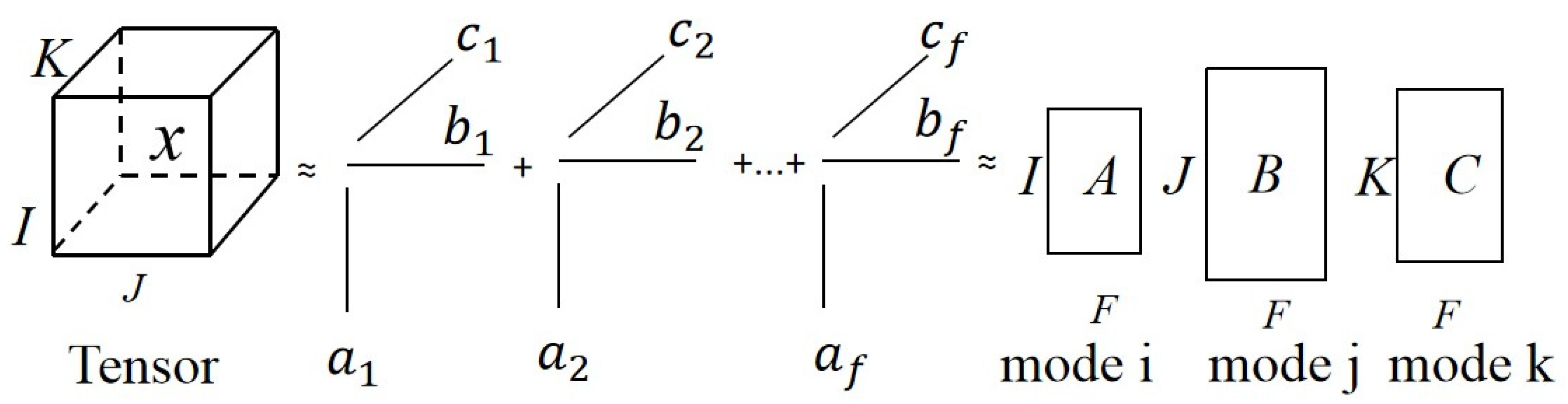
2.1. Principle of PARAFAC

PARAFAC analysis is a psychometrically derived multi-dimensional data decomposition method for any data set that can be described in more than two dimensions (e.g., temporal, spatial, frequency, participant, condition, signal features) and that facilitates the extraction of the different features present [25]. By using the algebraic characteristics and diversity characteristics of the signal, PARAFAC can obtain the required parameters to characterize the characteristics from the fitting of the multi-dimensional data set. It assumes that there is a multi-linear relationship between each independent parameter and that certain constraint conditions are identifiable via the decomposition of the matrices. In the traditional two-dimensional matrix, $x_{i,j}$ denotes the component in row i and column j. Extension to three-dimensional tensors leads to another index of “high” value (expressed in K). All the elements in the three-dimensional tensor are uniquely determined by $x_{i,j,k}$. The three-dimensional tensor is treated as a cube in which each element has three degrees of freedom. Fixing one degree of freedom determines a sub-matrix which can be regarded as making a section along a certain direction of the cube. Rank is used to reflect the correlation between the rows, columns, and heights of the matrix. In order to remove redundancy and reduce the parameters’ weight, the multi-dimensional tensor is decomposed by a low rank. The element in the tri-linear tensor $X\in C^{I\cdot J\cdot K}$ is assumed to be $x_{i,j,k}$, for which $i=1,\cdots ,I; j=1,\cdots ,J; k=1,\cdots ,K$. The trilinear tensors are decomposed into the form of the cross-product of a two-dimensional array, as shown below:

$$X=a_1•b_1•c_1+\cdots +a_R•b_R•c_R={\displaystyle \sum _{r=1}^R{a}_r•b_r•c_r}$$

(1)

where $a_r\in C^I$, $b_r\in C^J$, $c_r\in C^K$, and $r=1,\cdots ,R$. $•$ denotes the tensor product. R is the rank of the tensor $X$. The low-rank splitting of the tri-linear tensor was the decomposition model and is named PARAFAC. The decomposition process is shown in Equation (2):

$$S_{dft}={\displaystyle \sum _{k=1}^{N_k}{a}_{dk}{b}_{dk}{c}_{dk}+e_{dft}}$$

(2)

The processing objects in this research constitute the data matrix $S_{\left(N_d\cdot N_f\cdot N_t\right)}$. $N_d$, $N_f$, and $N_t$, which are composed of vibration signals by wavelet transform, are expressed as channels, frequency step size, and data points, respectively. The tensor is expanded with three-dimensional diversity, as shown in Figure 1 below.

The structure for achieving the strong identification results consists of the two-dimensional matrices $A, B$ and $C$, and is made of the vectors $a_k=\left\{a_{dk}\right\}$, $b_k=\left\{b_{fk}\right\}$ and $c_k=\left\{c_{tk}\right\}$ which are the spatial signal, spectral signal, and time signal of each atom. The variable $e_{dft}$ represents the error. By satisfying the equation $\mathrm{rank}\left(A\right)+\mathrm{rank}\left(B\right)+\mathrm{rank}\left(C\right)\ge 2N_k+2$, it is guaranteed that the matrices $\mathrm{A},\mathrm{B}$and $\mathrm{C}$ have identifiability and the decomposition of Formula (2) is achieved by solving (3), in which the vectors $a_{k\left(N_d\times 1\right)}$, $b_{k\left(N_f\times 1\right)}$, and $c_{k\left(N_t\times 1\right)}$ represent the k-th components of the space, spectrum, and time signals, respectively:

$$\min \Vert {\widehat{S}}_{dft}-{\displaystyle \sum _{k=1}^{N_k}{a}_{dk}{b}_{fk}{c}_{tk}}\Vert$$

(3)

$${\widehat{S}}_{dft}={\displaystyle \sum _{k=1}^{N_k}{a}_{dk}{b}_{fk}{c}_{tk}}$$

(4)

The PARAFAC model is decomposed with the trilinear least squares algorithm. The specific procedures are as follows:

(1)

Multi-dimensional analysis of time–frequency signal;

(2)

Set the values of component f;

(3)

Set the initial loading for two-dimensional arrays $B$ and $C$;

(4)

Estimate matrix $A$ with the least mean square. The formula is $A=X{Z}^{’}{(Z{Z}^{’})}^{-1}$, $Z=(b\otimes c)$;

(5)

Calculate B and C;

(6)

Return to step (4) and repeat the continuous calculation until convergence is achieved.

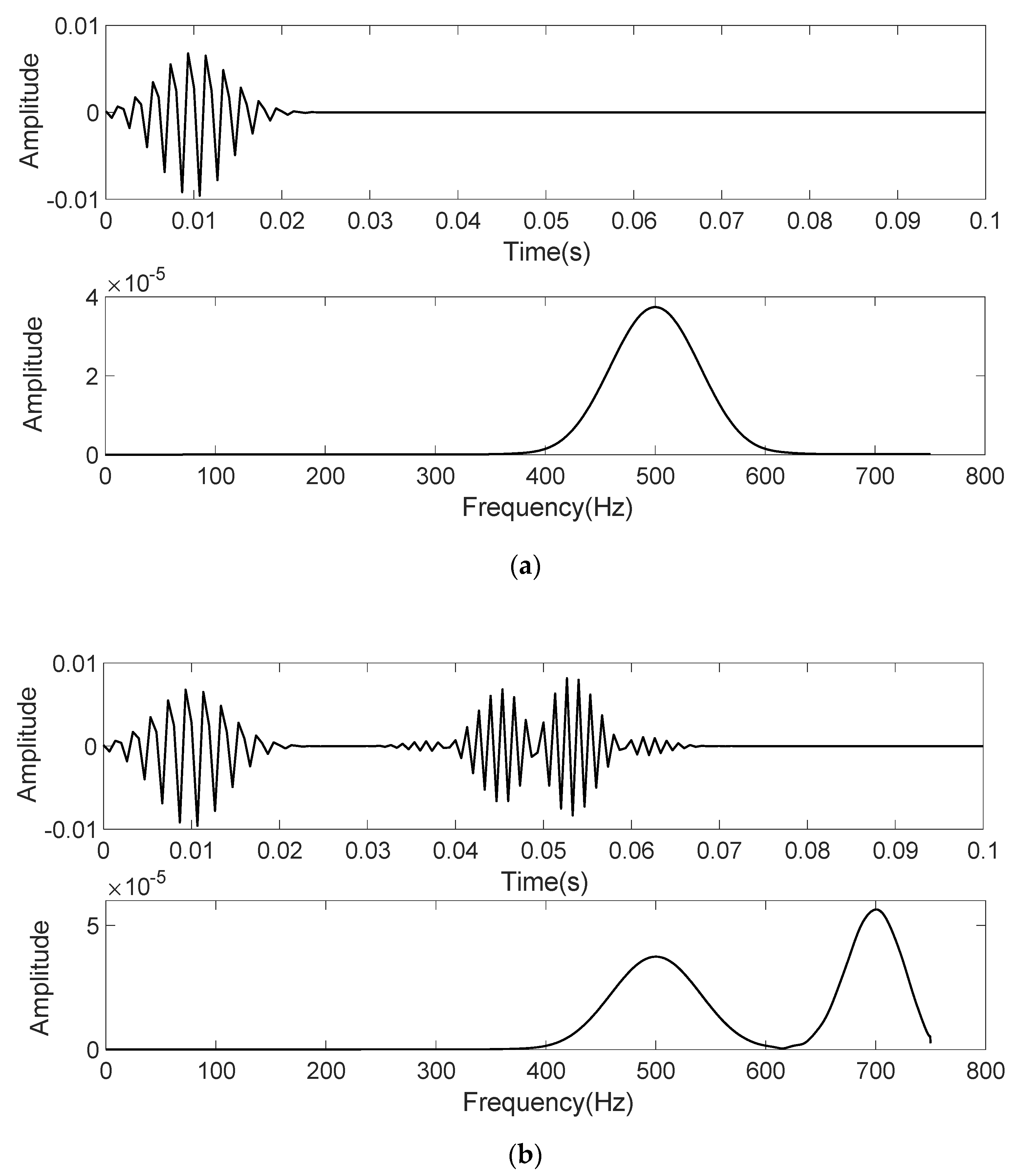
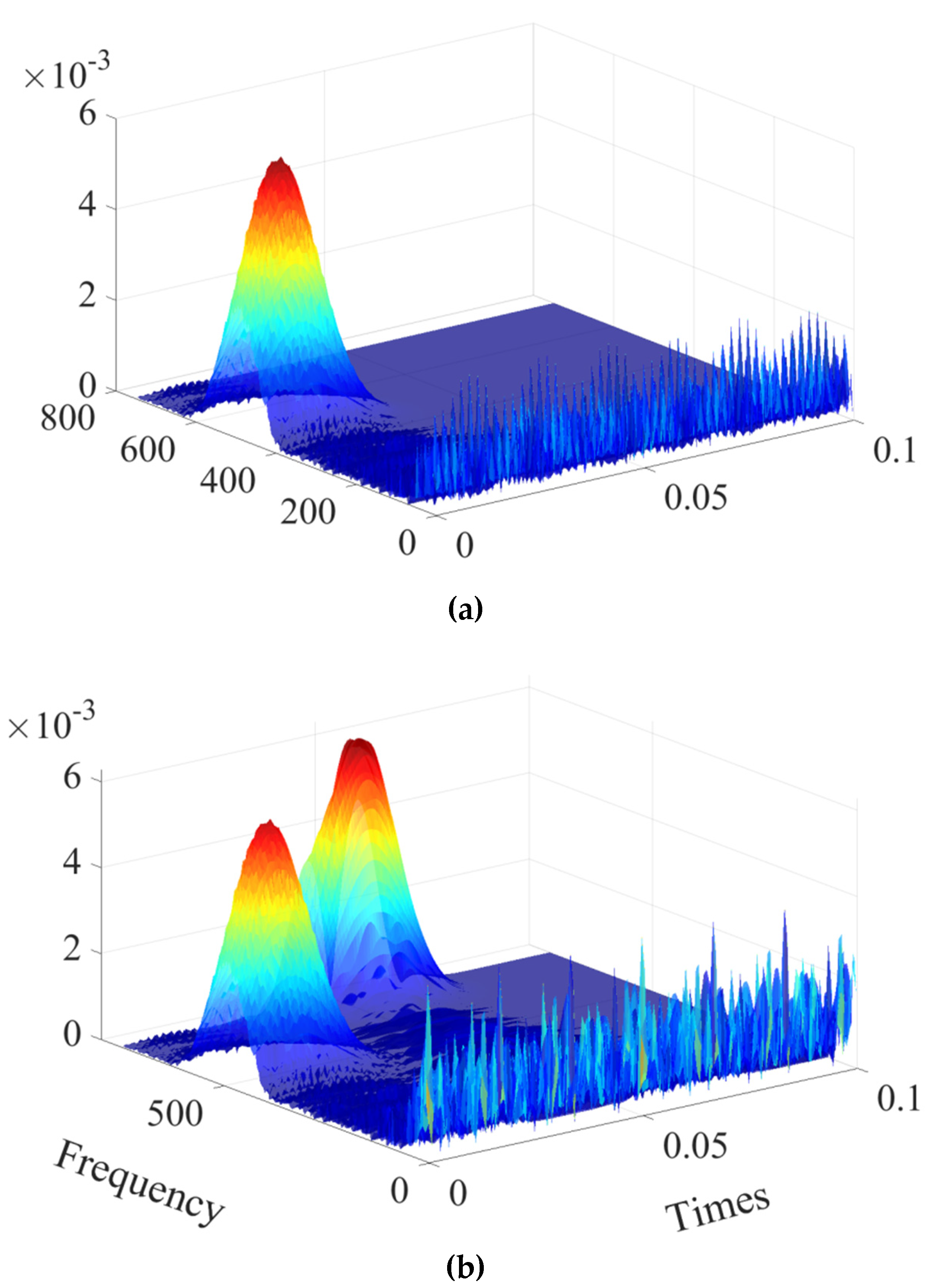
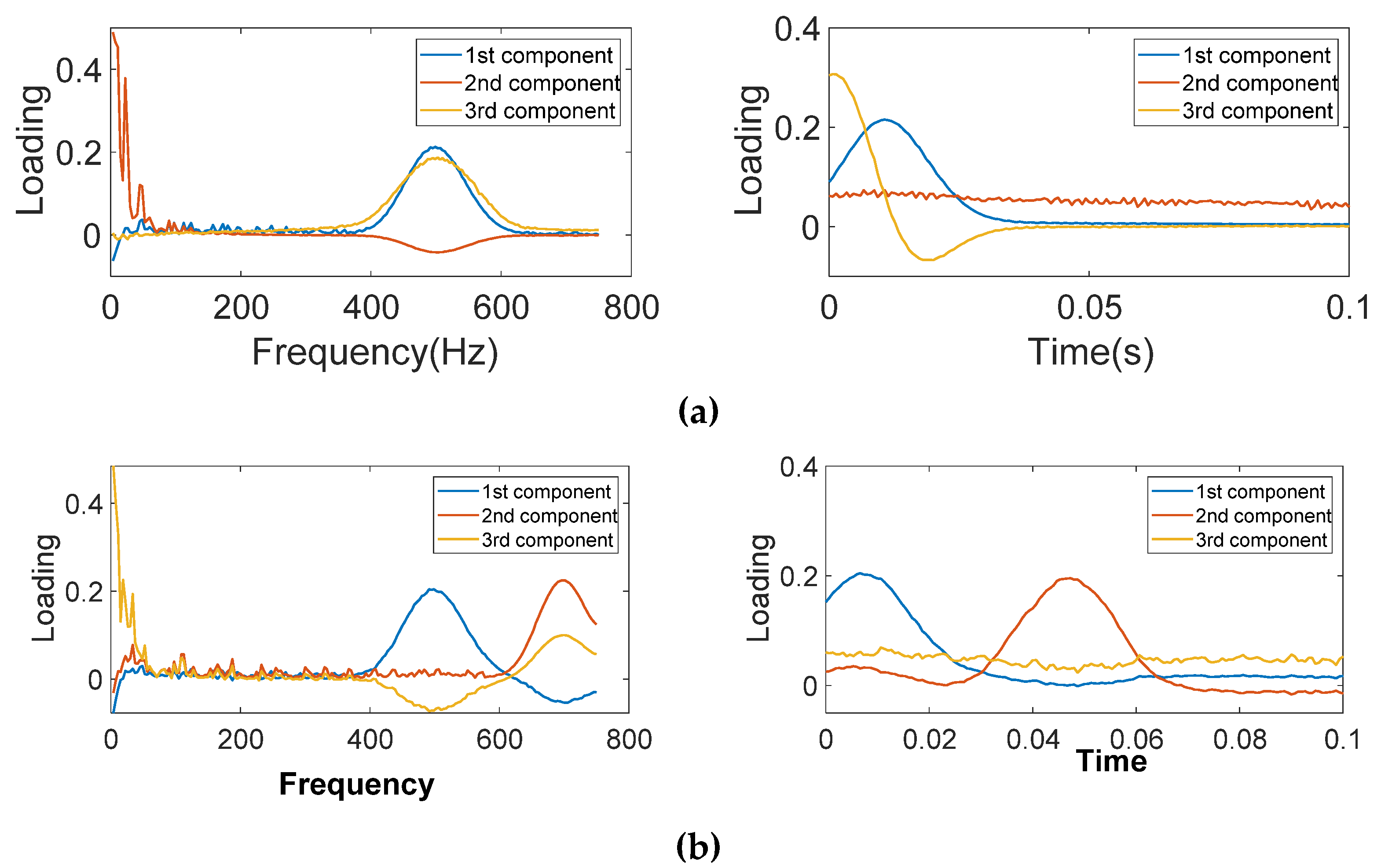
2.2. Algorithm Testing by Numerical Simulation

A simulation test was carried out on the simulation signal. The normal and fault simulation signals are as follows:

$$Y_1\left(t\right)=0.01\cos \left(1000\pi t-5\right)e^{-\frac{25{\left(100t-1\right)}^2}{8}}$$

(5)

$$Y_2\left(t\right)=0.01\cos \left(1000\pi t-5\right)e^{-\frac{25{\left(100t-1\right)}^2}{8}}+ 0.01\cos (1400\pi t-5)e^{-\frac{25{\left(100t-5\right)}^2}{18}}$$

(6)

In Figure 2, the variation law in relation to the amplitudes of the simulated signal with the time and frequency is demonstrated. Figure 3 shows the distribution of the signal in a three-dimensional spectrum after wavelet transform analysis. According to the analysis in Figure 2 and Figure 3, the corresponding frequency of the wave crest under normal conditions is 500 Hz, while the fault signal simulated by the simulation signal has two frequencies, 500 and 700 Hz. The frequency of 700 Hz is considered to be the main frequency containing fault information, and it is inferred that there is a fault simulation signal in the frequency range of 600–750 Hz.

After being transformed by the continuous wavelet, the simulation data were processed by the PARAFAC algorithm to establish the frequency, time, and channel factor decomposition. Figure 4 shows the comparison of the frequency characteristic matrix and the time characteristic matrix of the normal and fault signals. In the frequency decomposition signal of the normal signal, it can be observed that the amplitudes of the three components appear at the frequency of 500 Hz, and the frequency decomposition signal of the fault signal also shows amplitude changes at 500 and 700 Hz. The time information when the fault occurs can also be presented within the decomposition signal in the time domain. The methodology of the fault condition monitoring proposed in this paper is thus verified as effective.

3. PNN Parameter Optimization with IPSO

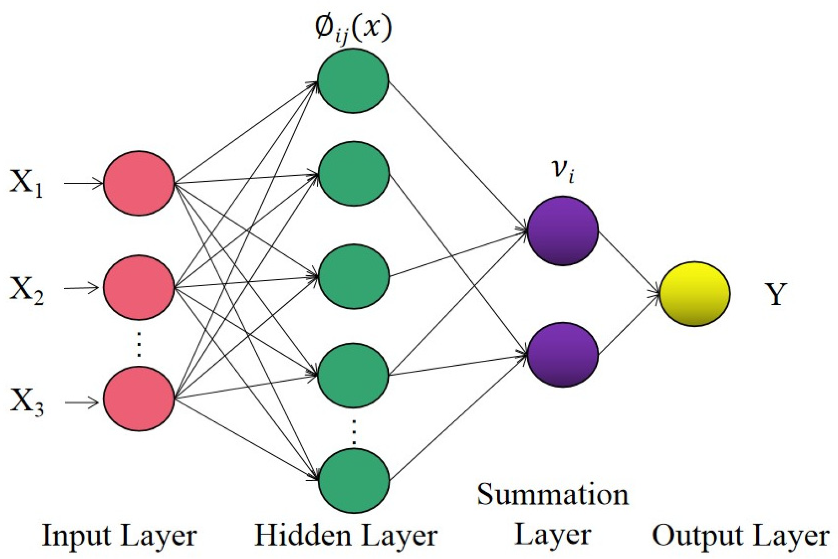
3.1. Principle of PNN

Probabilistic neural networks (PNNs) have high training efficiencies and can easily capture characteristics across signals. They have been widely used in pattern classification [26]. A PNN is an artificial neural network based on statistical principles, probability density estimation, and Bayesian decision theory. In some cases, a PNN can achieve arbitrary nonlinear transformation, and the final judgment extracted by this type of feed forward network converges towards the Bayesian optimal solution [27].

The structure of a PNN is made of an input level, a sample level, a summation level, and a competitive level, as seen in Figure 5.

The value of the feature samples is received by the network through the input layer, and the amount of feature value corresponds to the amount of input layers. The sample layer is used to calculate the probability needed to obtain the distance between each vector and neuron, and it then outputs the matching degree with a Gaussian function. In the sample layer, the amount of the neurons is equal to the amount of input used for training the sample vectors. The j-th neuron of the i-th mode in the sample level affects the mapping between the input vector $X$ and the output value $Y$. Equation (7) is the definition formula:

$${\Phi }_{ij}\left(x\right)=\frac{1}{{\left(2\pi \right)}^{1/2}{\sigma }^d}{e}^{-\frac{\left(x-x_{ij}\right){\left(x-x_{ij}\right)}^T}{{\sigma }^2}}$$

(7)

In the expression, $i=1,2,\cdots ,m$, $m$ is the total class amount of samples, $d$ represents the dimensions of the array, and the smoothing parameter is $\sigma$, which is the only adjustable parameter for improving the network accuracy, generally between 0 and 1. $x_{ij}$ represents the $i$ data of the $j$ sample. The summation layer further divides the sample layer, and the pattern units belonging to the same class are classified and integrated into the neurons of this layer, so the amount of neurons is equal to the amount of classifications. By calculating the weighted average of the outputs of each type of hidden neuron in the sample layer, the category of the input vector is obtained by the following equation:

$${\nu }_i=\frac{{\displaystyle \sum _{j=1}^L{\Phi }_{ij}}}{L}$$

(8)

The variable $v_i$ denotes the output of class $i$and $L$ denotes the amount of neurons of class $i$. The largest category in the summation layer is filtered by the competitive layer as the output category:

$$y=\arg \max \left({\nu }_i\right)$$

(9)

3.2. Improving the Particle Swarm Optimization Algorithm

As a traditional intelligent algorithm, PSO has strong advantages in dealing with complex optimization problems, but it has the disadvantages of premature convergence and difficult constraints. Therefore, the authors adopted an IPSO algorithm to give a precise determination of the super smooth parameters of a PNN. Based on the PSO algorithm shown in Equations (10) and (11), the new dynamic inertia weight and the optimized particle velocity and position update strategy are introduced to stop the algorithm performing local optimization, which enhances the generalization performance of the SVM model [28]:

$${\nu }_{id}^k={\omega }_i{\nu }_{id}^{k-1}+c_1{r}_1\left(p_{bi}-x_{id}^{k-1}\right)+c_2{r}_2\left(p_g-x_{id}^{k-1}\right)$$

(10)

$$x_{id}^k=x_{id}^{k-1}+{\nu }_{id}^k$$

(11)

Here, the parameter $i=1,2,\cdots ,m$, and $d=1,2,\cdots ,n$, for which $m$ denotes the size of the particles; the parameter $n$ is the dimension of the solution vector space; the parameters $c_1$ and $c_2$ are two normal numbers; and the parameters $r_1$ and $r_2$ are two independent random numbers in the range of (0, 1). ${\omega }_i$ represents the momentum term coefficient, $p_{bi}$ represents the optimal position experienced by the current particle, and $p_g$ represents the optimal position in the whole population.

The construction of the IPSO algorithm suggested in this thesis benefits from the improvement of the traditional PSO algorithm in the following two aspects:

(1) An IPSO algorithm is proposed in which the influence of the other particles of the population on the particle optimization is considered in the iteration. The velocity of each particle in the solution space is trained in real time based on three factors of its own optimal solution $p_{bi}$, neighborhood optimal solution $q_b$, and global optimal solution $p_g$.

In the iteration, the distance between each particle and the other particles is calculated, the distance $l_{mn}$ between the current $m$ particle and any particle $n$ is recorded, the maximum distance is $l_{\max }$, and the ratio is calculated with $\raisebox{1ex}{$l_{mn}$}\!\left/ \!\raisebox{-1ex}{$l_{\max }$}\right.$. The threshold value changes according to the number of iterations $k$, and its expression is:

$$\xi =\frac{0.3k+0.6k_{\max }}{k_{\max }}$$

(12)

The maximum number of iterations is the set value $k_{\max }$. When $\xi <0.9$, if $\raisebox{1ex}{$l_{mn}$}\!\left/ \!\raisebox{-1ex}{$l_{\max }$}\right.<\xi$, the $n$ particle is considered to be in the neighborhood of the $m$ particle. Accordingly, a new learning factor $c_3$ and a random number $r_3$ are introduced to update the particle velocity according to the following formula:

$${\nu }_{id}^k={\omega }_i{\nu }_{id}^{k-1}+c_1{r}_1\left(p_{bi}-x_{id}^{k-1}\right)+c_2{r}_2\left(p_g-x_{id}^{k-1}\right)+c_3{r}_3\left(q_b-x_{id}^{k-1}\right)$$

(13)

If $\xi >0.9$ or if the ratio $\raisebox{1ex}{$l_{mn}$}\!\left/ \!\raisebox{-1ex}{$l_{\max }$}\right.>\xi$, the particle velocity is updated according to Equation (10).

(2) The standard PSO algorithm uses a linear reduction of ${\omega }_i$ to reduce the search step size and make the iteration gradually converge to the extreme point. The disadvantage of this method is that the algorithm is excessively sensitive and can easily enter the local optimal solution. In order to improve the global convergence capability, the parameter ${\omega }_i$ is reduced by the $S$ shape function; that is, ${\omega }_i$ changes dynamically. When the search has started, the value of ${\omega }_i$ is convenient for the global search, and when the search process is close to the end, the value of ${\omega }_i$ becomes smaller, which is conducive to the local search. The weight expression in the IPSO algorithm is as follows:

$$\omega =\frac{{\omega }_{\max }-{\omega }_{\min }}{1+\exp (2e\cdot t/t_m-e)}$$

(14)

The procedure of the IPSO algorithm is developed as such:

Step 1: Determine the relevant parameters of IPSO, such as the learning factor, particle swarm size, and upper limit of iterations;

Step 2: Assume that the best position in history that the particle has experienced is $p_{bi}=\left(x_{i1},x_{i2},\dots ,x_{in}\right)$, the corresponding extreme value is $p_{bf}$, the global extreme value position is $p_{gi}=\left(x_{g1},x_{g2},\dots ,x_{gn}\right)$, and the corresponding global extreme value is $p_{gf}$;

Step 3: Calculate all particle fitness values $p_i$;

Step 4: Compare and obtain $p_{bi}$, $p_{bf}$, $p_g$, $p_{gf}$;

Step 5: Update the position of the particles within a limited range:

If $x_{ij}\left(k+1\right)>x_{\max }$, then $x_{ij}\left(k+1\right)=x_{\max }$.

If $x_{ij}\left(k+1\right)<x_{\min }$, then $x_{ij}\left(k+1\right)=x_{\min }$.

$x_{\max }$ and $x_{\min }$ are the maximum position and the minimum position, respectively;

Step 6: The iteration ends after the number of iterations or the cut-off accuracy is reached. Otherwise, return to step 2 to continue the calculation.

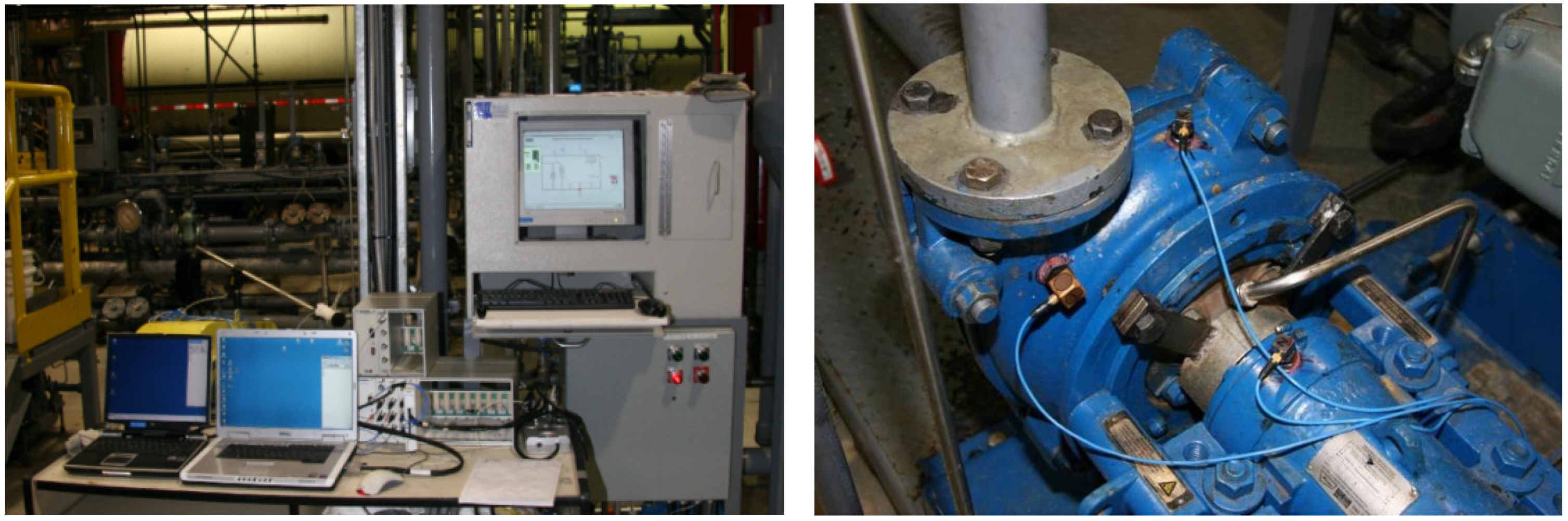
4. Experimental System

A centrifugal pump is a very complex nonlinear system. There are many reasons for the failure of a slurry pump. The common failures of the centrifugal pump impeller, including perforation damage to impeller F2, outer edge wear for impeller F3, and blade wear for impeller F4, are compared with the normal impeller F1.

For the purpose of acquiring the characteristic information data of the nonlinear multi-fault modes, the mechanical multi-source dynamic signal monitoring system was established, as shown in Figure 6. The system includes signal source acquisition and analysis systems such as the vibration signal, pressure signal, and flow signal, with respective motor speeds of 1200 rpm. The temperature, pressure, flow, vibration, and other signals can be locally displayed on the instrument through the multi-channel acquisition of the system to simulate the actual work of a nonlinear fault by altering the pressure and the flow of the mechanical state information.

The different running conditions of the slurry pump were simulated by replacing different impellers and changing the rotational speed, pressure, and flow. The vibration signals are collected by the accelerometers on three different positions that are on the chassis of the pump and outside the frame near the outlet and the bearing. The steps are as follows: (1) The normal centrifugal pump uses the normal impeller F1. We adjust the impeller speed to 1200 rpm. The experimental data are collected by the datal acquisition system. The data acquisition time of each group is 20 s and the acquisition frequency is 9 KHz; (2) We use F2, F3, and F4 to replace the set-up of the stable operating status, and repeat step 1 to collect the multi-source data such as vibration data, pressure data, and flow rate data.

5. PARAFAC-IPSO-PNN for Multi-Dimensional Data Analysis

The identification model for mechanical nonstationary multi-fault mode consists of PARAFAC and IPSO-PNN, as shown in Figure 7. The procedure of the classification model implementation is as follows: (1) The multi-channel vibration signals are collected by three accelerometers; (2) The vibration signals are transformed to be the representation of time–frequency by continuous wavelet; (3) The time–frequency domain data are used to construct the three-dimensional arrays; (4) The arrays are decomposed by the PARAFAC to obtain the time domain loading factors and frequency domain loading factors; and (5) The PARAFAC loading factors are used as features to be input to IPSO-PNN classifiers to obtain the modes.

The centrifugal pump system was tested. A total of 120 groups of data for the normal running conditions and the three fault conditions were acquired to identify the operation states of the slurry pump for fault diagnosis and classification. Ninety groups of vibration data from three accelerometers were input to train the fault diagnosis model as described in Figure 7. We obtained the fault diagnosis model for four operating conditions that were F1, F2, F3, and F4. Then, there were 10 groups of testing data for each operating condition. Forty groups of testing data were input to the trained fault diagnosis model to obtain mode category.

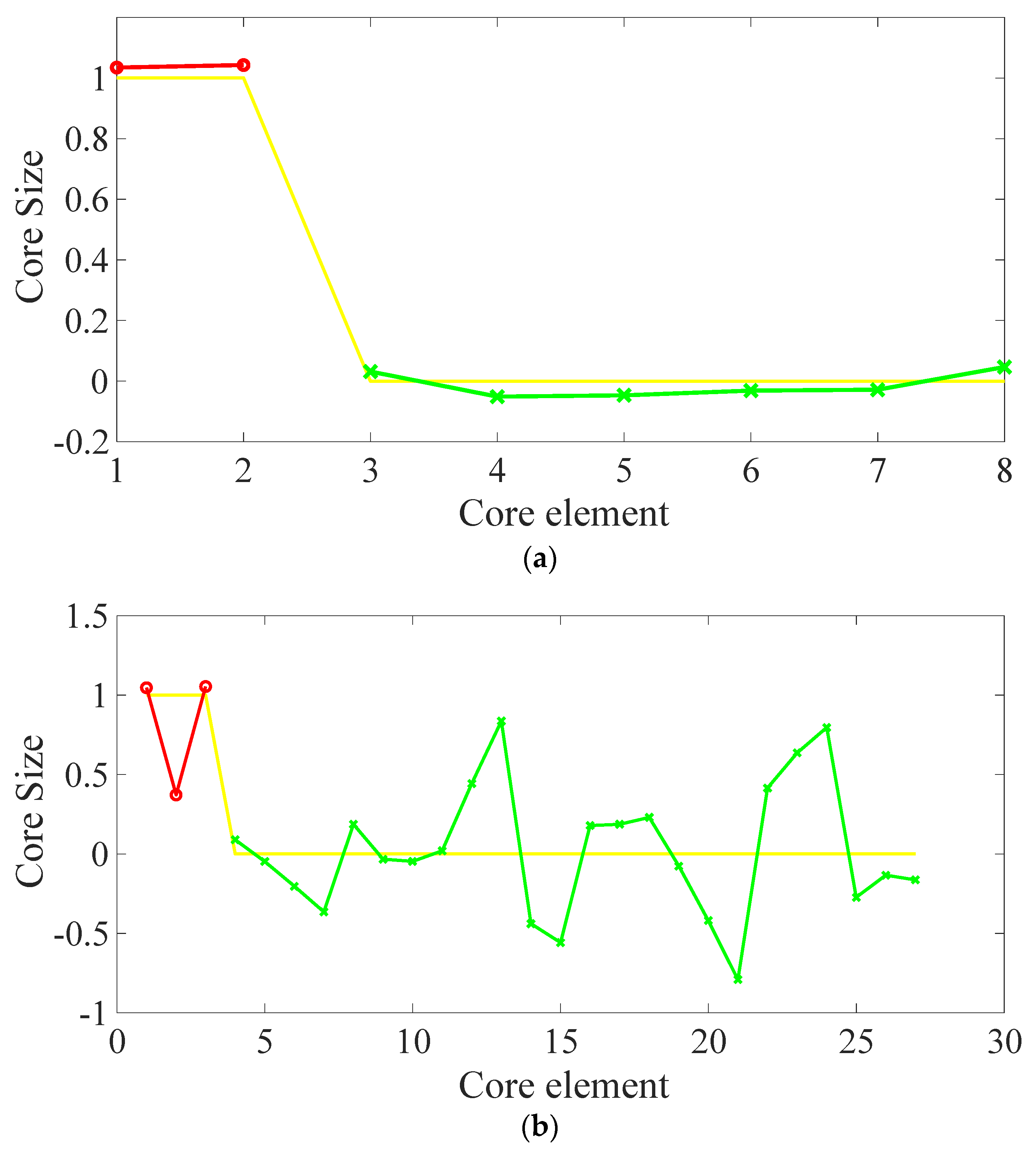
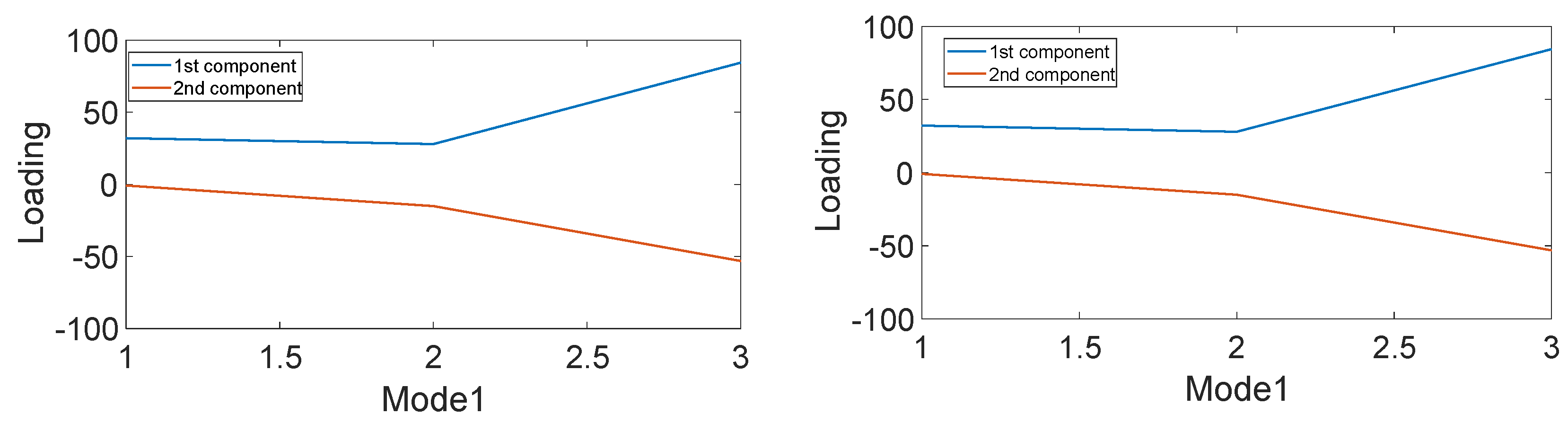
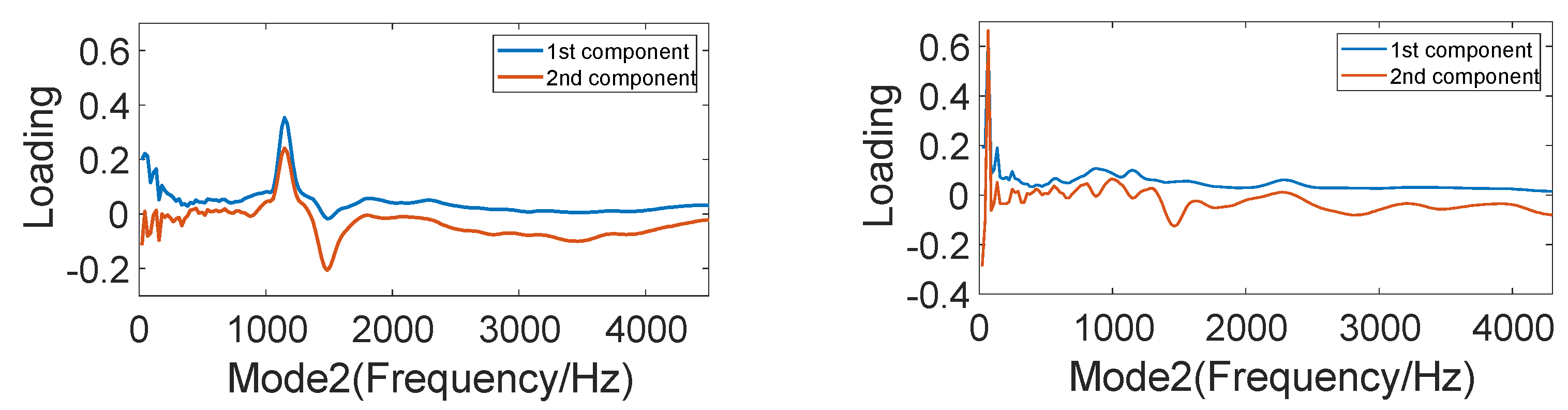
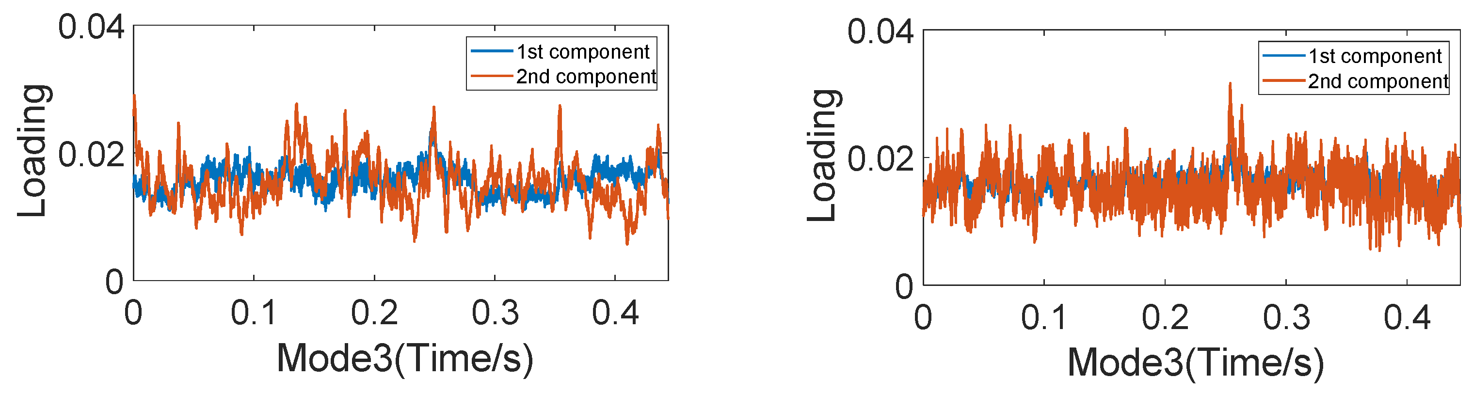
5.1. PARAFAC for Data Decomposition

The objective of the optimized probabilistic neural network model was to explore the data processing ability. The performance after the different fault characteristic signals were input was tested, the time–frequency features extracted by the PARAFAC decomposition of multi-source signals were calculated by the PNN model and the IPSO-PNN model as feature parameters. The classification accuracy of the two models was compared. The corresponding states of the PNN model output and the centrifugal pump are shown in

Table 1. Neural network output corresponding to each state of the centrifugal pump.

Pattern	F1	F2	F3	F4
Output of PNN	1	2	3	4

.

PARAFAC was used to process the test data. The algorithm can simultaneously integrate the three-way vibration signals of a single measuring point and the one-way vibration signals and flow signals of multiple measuring points in the data set. Then, a correct parallel factorization model was established with the nuclear consistency diagnosis. The factor number was two. The decomposition results are shown in the figure below. Figure 8a shows that the core consistency is 99.4% when the factor number equals 2. Figure 8b shows that the core consistency is 31.2% when the factor number equals 3. Here, the yellow line is the target, the green data should be zero, and red data are non-zero.

The PARAFAC algorithm requires the accuracy of factor F. Excessively high values of factor F would increase the model error. A meaningful solution can also not be obtained with excessively low values of factor F. The appropriate values of the factors can be determined according to the core consistency theory. Core consistency is the difference between the super diagonal array and the core three-dimensional data array in the constructed PARAFAC model. The theoretical basis for the ideal model is that the super diagonal array is completely consistent with the core data array. The low kernel consistency value indicates that the model deviates from trilinearity. When the value is greater than 60%, the model is considered to be close to trilinear. As shown in Figure 6, the kernel consistency is only 31.206% when the number of factors is 3. When the number of factors is 2, it is close to the ideal value. It can be judged that the appropriate number of factors is 2.

Figure 9, Figure 10 and Figure 11 show that the three-channel vibration signals are decomposed by PARAFAC to obtain the spatial loading factors, frequency loading factors, and time loading factors, which are used as feature values to be input to the PNN for training classifier models. We compared the PARAFAC analysis for the data under normal conditions (F1) and fault conditions (F2). It is demonstrated that the characteristics are different in terms of the frequency factors, as shown in Figure 10, and time factors, as shown in Figure 11. In Figure 10, the major difference of the loading factor is the peak frequencies, which are approximately 1000 Hz for F1 but low frequency components for F2. In Figure 11, the loading factors contain much more noise for F2 than that for F1. Based on the characteristic features in Figure 10 and Figure 11, the time and frequency loading factors are chosen as features for training the PNN models.

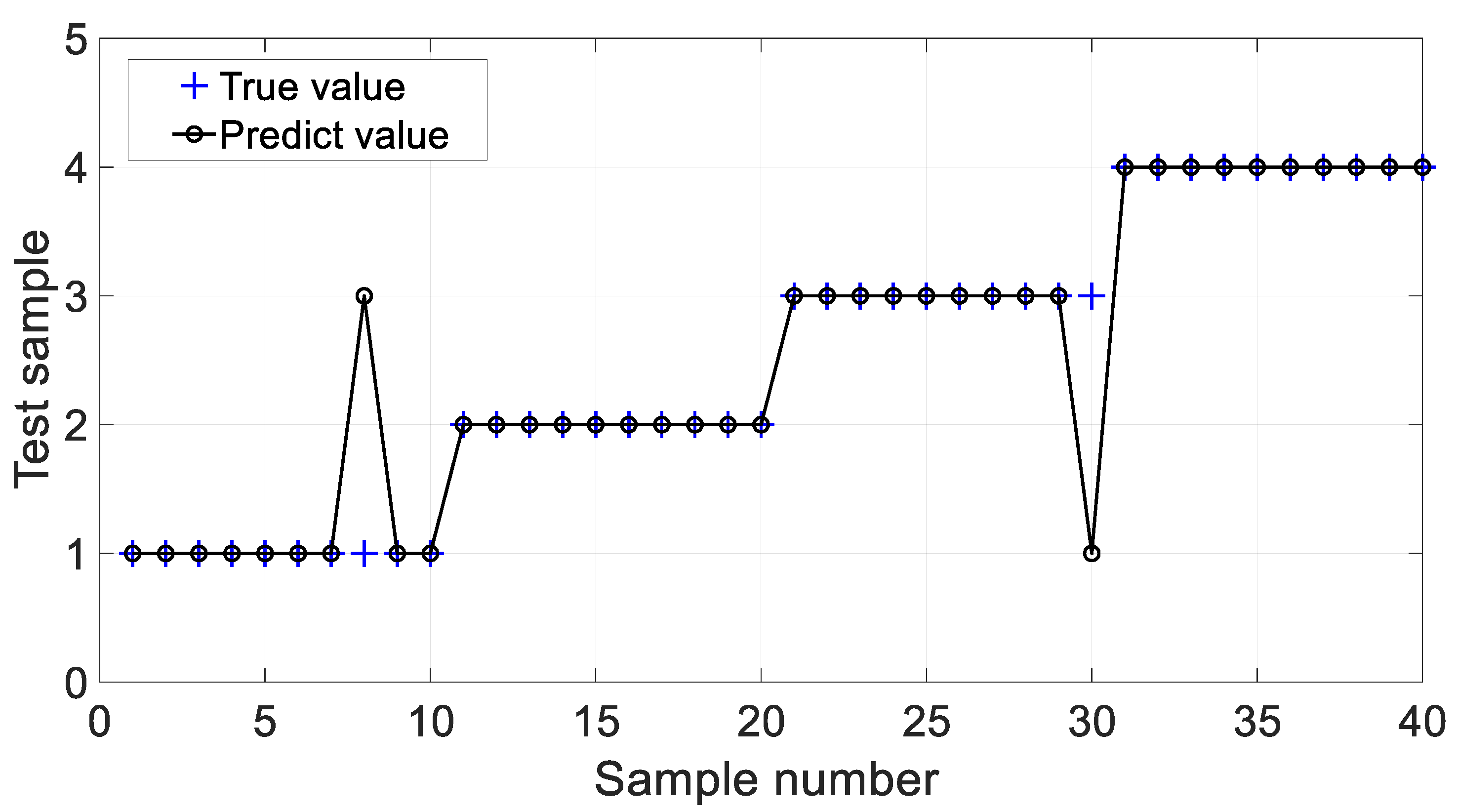
5.2. IPSO-PNN for Classification

The 40 groups of original data collected under four working conditions were divided into two: 30 groups as training samples versus 10 groups as test samples. For this example, the particle swarm size was set to 100, and iterations are performed 20 times. After PNN processing, the IPSO model is selected for further classification. To confirm the training effect of the IPSO-PNN classification model, the characteristic signals are input to the non-optimized and optimized neural network model to output the faulty categories. Figure 12 shows that there are two errors between the true value and predicted value. Figure 13 shows that there is one error between the true value and predicted value. By the comparison between Figure 12 and Figure 13, the IPSO is used to improve the performance of PNN for the identification of the data category. The IPSO-PNN is proposed as classifier to identify the operating status in the following section.

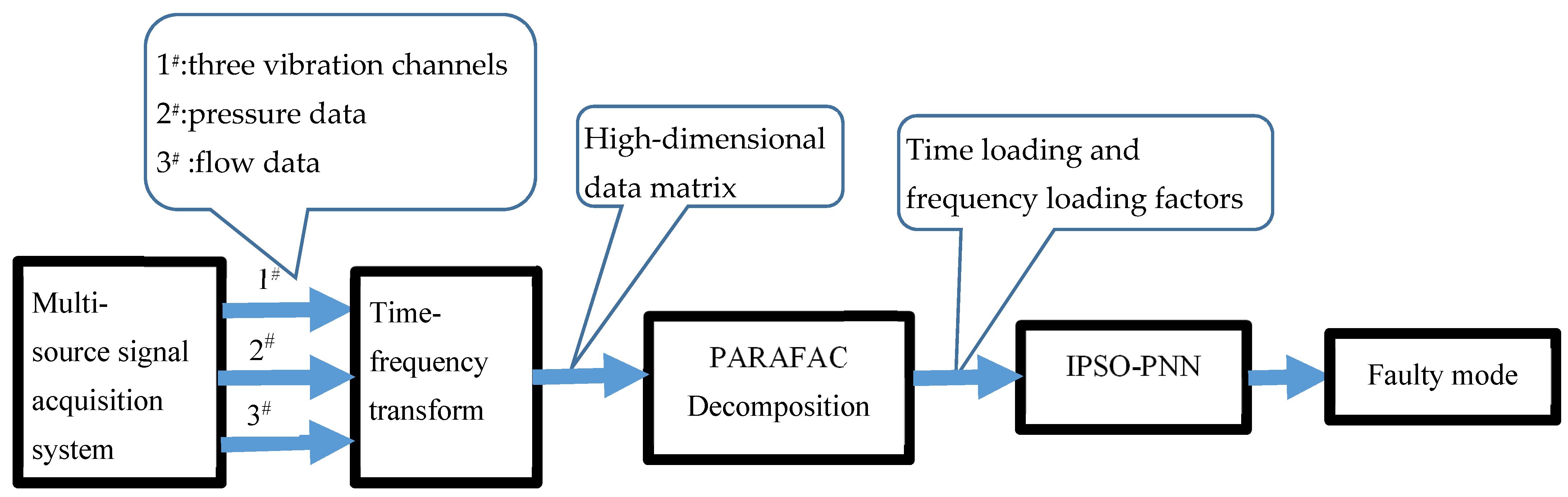
5.3. Multiple-Source Data Analysis for Classification

The vibration signals along the X axis directions of the three accelerometers from three measurement points are obtained, which are used as the data driven and signal processing by PARAFAC to calculate the features for classification. PNN and IPSO-PNN are used to recognize the PARAFAC atoms to identify the multiple fault modes of the slurry pump. The test set accuracy and running time are used to assess the capability of PNN and IPSO-PNN. As shown in

Table 2. Classification accuracy of the vibration signals of three sensors along x axis by PARAFAC.

	Test Set Accuracy	Time (s)
PNN	82.5%	0.125
IPSO-PNN	85%	0.026

, the classification accuracy by PNN and IPSO_PNN are 82.5% and 85%, which suffices to demonstrate the advantages of IPSO-PNN and the effectiveness of IPSO for optimizing and improving the capability of PNN. The running time of classification by IPSO-PNN is 0.026, which is much less than that of PNN—0.125 s. The IPSO-PNN has potential applications for the recognition of the slurry pump under online conditions due to the benefits of a shorter running time.

In this paper, we had the motivation to develop intelligent multiple-sensor signal analysis and fusion to diagnose the nonstationary fault multi-mode of mechanical system by making use of vibration data. The vibration data are excited by the oil sand in the pipeline of the oil sand transport system. The pressure and flow rate are enable the control over the operating status via parameters such as rotational speed, which is the source of the generation source of the chassis vibration of slurry pump. We hope to develop PARAFAC to handle multi-dimensional data including the causing source data and corresponding resulting response data, which are supposedly contain abundant information including both sensitive and insensitive data on the faulty component of slurry pump. PARAFAC has the strong advantage of processing multi-source high-dimensional system data. There are five sensors that provide the five-channel data which are three vibration sensors, one pressure sensor, and one flow sensor. The PARAFAC was designed to be a data-driven methodology that processes multi-sensor data by constructing the three dimensional signal representation. Multi-dimensional data analysis based on the PARAFAC theory algorithm is used to eliminate irrelevant and redundant components in signals and reveal the important characteristic information required, which establishes the intrinsic matching relationship among the vibration, pressure, and flow data sources. It is just because of reducing the irrelevant information distortion effects of inter-channel interaction on the intrinsic features that is excited by the fault mode mechanism that the classification accuracy is improved by PARAFAC in comparison to PNN and IPSO. Additionally, the more data sources it has, the stronger capability in classification accuracy the PARAFAC has.

Table 3. Classification accuracy of the vibration, pressure, and flow signals of five sensors by PARAFAC.

	Test Set Accuracy	Time (s)
PNN	95%	0.033
IPSO-PNN	97.5%	0.025

shows the three vibration sensors, one pressure sensor, and one flow sensor signal fusion by PARAFAC. The classification accuracy with five-source data analysis with PARAFAC is 95% with PNN and 97.5% with IPSO-PNN. It is demonstrated that the 95% classification accuracy with the analysis of data from five sources by PNN is higher than that of 82.5% which is obtained with the analysis of data from three sources by PNN. The 97.5% classification accuracy with five sources’ data analysis by IPSO-PNN is higher than that of 85% obtained by the analysis of data from three sources by IPSO-PNN. This definitely verifies that IPSO effectively increases the classification accuracy by comparison between PNN and IPSO-PNN, as shown in Table 2 and Table 3. It also definitely verifies that the data fusion by the vibration, pressure, and flow, is much better than that which just has vibration data by comparison between the classification accuracy in Table 2 and Table 3.

6. Conclusions

The parallel factor algorithm was studied by applying the advantages of PARAFAC in multi-source data information processing under the condition monitoring of the centrifugal pump. The PNN algorithm is optimized by the IPSO algorithm, which has achieved good results in fault diagnosis. Compared with the traditional time–frequency domain processing methods, the PARAFAC algorithm characteristically analyzes multi-dimensional data information, processes complex signals, removes redundant signals, and retains the important features. Compared with PNN, the classification accuracy of the optimized PNN is significantly improved and is of greater value for future applications. The analysis of many more data sources by combing the vibration, pressure, and flow is only superior to the analysis of vibration data of a slurry pump in multi-fault mode, which was strongly verified. In future research, the parameters of the fault diagnosis model must undergo further optimization to achieve correction rates of 100%.

References

1. Jiao, J.; Zhao, M.; Lin, J.; Liang, K. Hierarchical discriminating sparse coding for weak fault feature extraction of rolling bearings. Reliab. Eng. Syst. Saf. 2019, 184, 41–54. [Google Scholar] [CrossRef]
2. Lei, Y.G.; He, Z.J. Advances in applications of hybrid intelligent fault diagnosis and prognosis technique. J. Vib. Shock. 2011, 30, 129–135. [Google Scholar]
3. Shao, H.; Cheng, J.; Jiang, H.; Yang, Y.; Wu, Z. Enhanced deqgated recurrent unit and complex wavelet packet energy momententropy for early fault prognosis of bearing. Knowl.-Bascd Syst. 2020, 188, 105022. [Google Scholar]
4. Yang, L.; Chen, H.; Ke, Y.; Li, M.; Huang, L.; Miao, Y. Multi-source and multi-fault condition monitoring based on parallel factor analysis and sequential probability ratio test. EURASIP J. Adv. Signal Process. 2021, 2021, 1–33. [Google Scholar] [CrossRef]
5. Sun, G.; Zhang, Y. Development of Mechanical Equipment Fault Diagnosis System Based on Big Data Technology. J. Phys. Conf. Ser. 2020, 1648, 4. [Google Scholar] [CrossRef]
6. Wang, M.; Zhang, Z.; Li, K.; Si, C.; Li, L. Survey on Advanced Equipment Fault Diagnosis and Warning Based on Big Data Technique. J. Phys. Conf. Ser. 2020, 1549, 4–5. [Google Scholar] [CrossRef]
7. Chen, H.; Shang, Y.; Sun, K. Multiple fault condition recognition of gearbox with sequential hypothesis test. Mech. Syst. Signal Process. 2013, 40, 469–482. [Google Scholar] [CrossRef]
8. Yang, L.; Chen, H.; Ke, Y.; Huang, L.; Wang, Q.; Miao, Y.; Zeng, L. A novel time–frequency–space method with parallel factor theory for big data analysis in condition monitoring of complex system. Int. J. Adv. Robot. Syst. 2020, 17, 1729881420916948. [Google Scholar] [CrossRef] [Green Version]
9. Chen, H.; Fan, D.; Huang, J.; Huang, W.; Zhang, G.; Huang, L. Finite element analysis model on ultrasonic phased array technique for material defect time of flight diffraction detection. Sci. Adv. Mater. 2020, 12, 665–675. [Google Scholar] [CrossRef]
10. Yang, Z.; Chai, Y. A survey of fault diagnosis for onshore grid-connected converter in wind energy conversion systems. Renew. Sustain. Energy Rev. 2016, 66, 345–359. [Google Scholar] [CrossRef]
11. Chen, H.; Fan, D.L.; Fang, L.; Huang, W.; Huang, J.; Cao, C.; Yang, L.; He, Y.; Zeng, L. Particle Swarm Optimization Algorithm with Mutation Operator for Particle Filter Noise Reduction in Mechanical Fault diagnosis. Int. J. Pattern Recognit. Artif. Intell. 2019, 34, 2058012. [Google Scholar] [CrossRef]
12. Azamfar, M.; Singh, J.; Bravo-Imaz, I.; Lee, J. Multisensor data fusion for gearbox fault diagnosis using 2-D convolutional neural network and motor current signature analysis. Mech. Syst. Signal Process. 2020, 144, 106861. [Google Scholar] [CrossRef]
13. Zhao, P. Research on Vibration Fault Diagnosis Method and System Implementation of Centrifugal Pump. Ph.D. Thesis, North China Electric Power University, Beijing, China, 2011. [Google Scholar]
14. Tong, Z.M.; Xin, J.G.; Tong, S.G.; Yang, Z.Q.; Zhao, J.Y.; Mao, J.H. Internal flow structure fault detection, and performance optimization of centrifugal pumps. Appl. Phys. Eng. 2020, 21, 85–117. [Google Scholar] [CrossRef]
15. Chen, H.; Miao, Y.; Chen, Y.; Fang, L.; Zeng, L.; Shi, J. Intelligent Model-based Integrity Assessment of Nonstationary Mechanical System. J. Web Eng. 2021, 20, 253–280. [Google Scholar] [CrossRef]
16. Jiang, W.; Li, Z.; Zhang, S.; Wang, T.; Zhang, S. Hydraulic Pump Fault Diagnosis Method Based on EWT Decomposition Denoising and Deep Learning on Cloud Platform. Shock Vib. 2021. [Google Scholar] [CrossRef]
17. Li, Z.; Jiang, W.; Zhang, S.; Sun, Y.; Zhang, S. A Hydraulic Pump Fault Diagnosis Method Based on the Modified Ensemble Empirical Mode Decomposition and Wavelet Kernel Extreme Learning Machine Methods. Sensors 2021, 21, 2599. [Google Scholar] [CrossRef]
18. Abdi, A.; Emamian, E.S. Fault diagnosis engineering in molecular signaling networks: An overview and applications in target discovery. Chem. Biodivers. 2010, 7, 1111–1123. [Google Scholar] [CrossRef]
19. Guo, X. Research on Online Monitoring and Fault Diagnosis Method of Electric Motor and Centrifugal Pump Set. Ph.D. Thesis, Beijing University of Chemical Technology, Beijing, China, 2020. [Google Scholar]
20. Nie, J. Research on Centrifugal Pump Fault Diagnosis Method Based on Support Vector Machine. Ph.D. Thesis, Harbin Institute of Technology, Harbin, China, 2017. [Google Scholar]
21. Yang, C. Research on the Application of Parallel Factor Analysis in Blind Separation of Multiple Fault Sources. Ph.D. Thesis, Nanchang University of Aeronautics, Nanchang, China, 2018. [Google Scholar]
22. Li, J.F.; Zhang, S.F. Joint angular and Doppler frequency estimation of dual-base MIMO radar based on quadratic linear decomposition. J. Aeronaut. 2012, 33, 1474–1482. [Google Scholar]
23. Nion, D.; Sidiropoulos, N.D. A PARAFAC-based technique for detection and localization of multiple targets in a MIMO radar system. In Proceedings of the 2009 IEEE International Conference on Acoustics, Speech and Signal Processing, Taipei, Taiwan, 19–24 April 2009; pp. 2077–2080. [Google Scholar] [CrossRef]
24. Weis, M.; Romer, F.; Haardt, M.; Jannek, D.; Husar, P. Multi-dimensional space-time-frequency component analysis of event related EEG data using closed-form PARAFAC. In Proceedings of the 2009 IEEE International Conference on Acoustics, Speech and Signal Processing, Taipei, Taiwan, 19–24 April 2009; pp. 349–352. [Google Scholar] [CrossRef]
25. Ishii Stephanie, K.L.; Boyer Treavor, H. Behavior of reoccurring PARAFAC components in fluorescent dissolved organic matter in natural and engineered systems: A critical review. Environ. Sci. Technol. 2012, 46, 2006–2017. [Google Scholar] [CrossRef]
26. Feng, A.A. Research on Fault Diagnosis of Truck Bearings Based on Optimized Probabilistic Neural Network. Ph.D. Thesis, Beijing Jiaotong University, Beijing, China, 2019. [Google Scholar]
27. Li, K.; Tai, N.; Zhang, S. Fault monitoring of microtempered motor bearings based on wavelet packet entropy and probabilistic neural network. Micro Spec. Mot. 2016, 44, 37–39. [Google Scholar]
28. Fang, L.; Fan, D.; Zhang, G.; Chen, H. A particle swarm optimization particle filtering noise reduction algorithm with variational operators. J. Wuhan Univ. Eng. 2019, 41, 392–398. [Google Scholar]
Figure 1. Multiscale PARAFAC decomposition model.
Machines 10 00155 g001
Figure 2. (a) Simulation signal and spectrum by Equation (5). (b) Simulation signal and spectrum by Equation (6).
Machines 10 00155 g002
Figure 3. (a) The time-frequency representation of the simulated signal with Equation (5), (b) The time-frequency representation of the simulated signal with Equation (6).
Machines 10 00155 g003
Figure 4. (a) Frequency loading (Left) and time loading (Right) of the simulation signal with Equation (5). (b) Frequency loading (Left) and time loading (Right) of the simulation signal with Equation (6).
Machines 10 00155 g004
Figure 5. PNN network structure.
Machines 10 00155 g005
Figure 6. Centrifugal pump system with multi-source data acquisition.
Machines 10 00155 g006
Figure 7. Procedure about Fault diagnosis model of four operating conditions.
Machines 10 00155 g007
Figure 8. Nuclear consistency with factor numbers (a) F = 2 and (b) F = 3.
Machines 10 00155 g008
Figure 9. Comparison between the normal F1 Mode1 (Left) and fault F2 Mode1 (Right).
Machines 10 00155 g009
Figure 10. Comparison between the normal F1 Mode2 (Left) and fault F2 Mode2 (Right).
Machines 10 00155 g010
Figure 11. Comparison between the normal F1 Mode3 (Left) and fault F2 Mode3 (Right).
Machines 10 00155 g011
Figure 12. Comparison between the predicted and real values of PNN model classification.
Machines 10 00155 g012
Figure 13. Comparison between the predicted and real values of IPSO-PNN model classification.
Machines 10 00155 g013