
Indirect Estimation of Tire Pressure on Several Road Pavements via Interacting Multiple Model Approach

Abstract
:1. Introduction
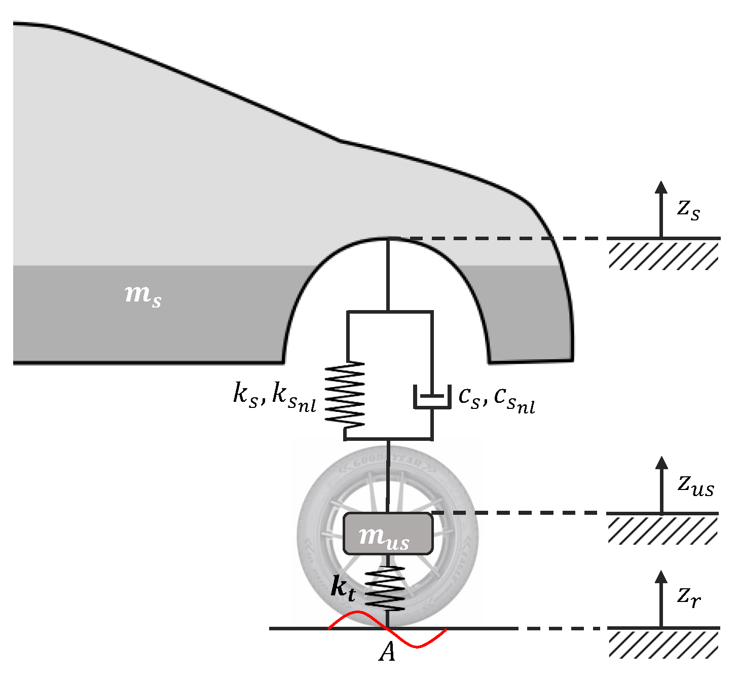
2. Vehicle Dynamics and Road Profile Synthesis Modelling
2.1. Road Surface Profile Synthesis
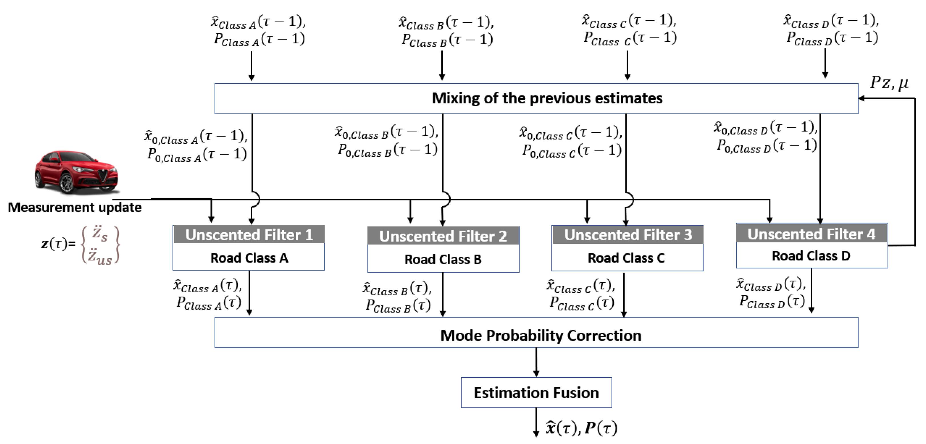
3. Interacting Multiple Model Filter
- 1.
- Mode Probability Prediction:
- 2.
- Mixing of the previous estimates:
- 3.
- Mode dependent UKFs, whose equations can be found in [34].
- 4.
- Mode Probability Correction:
- 5.
- IMMUF’s corrected estimates:
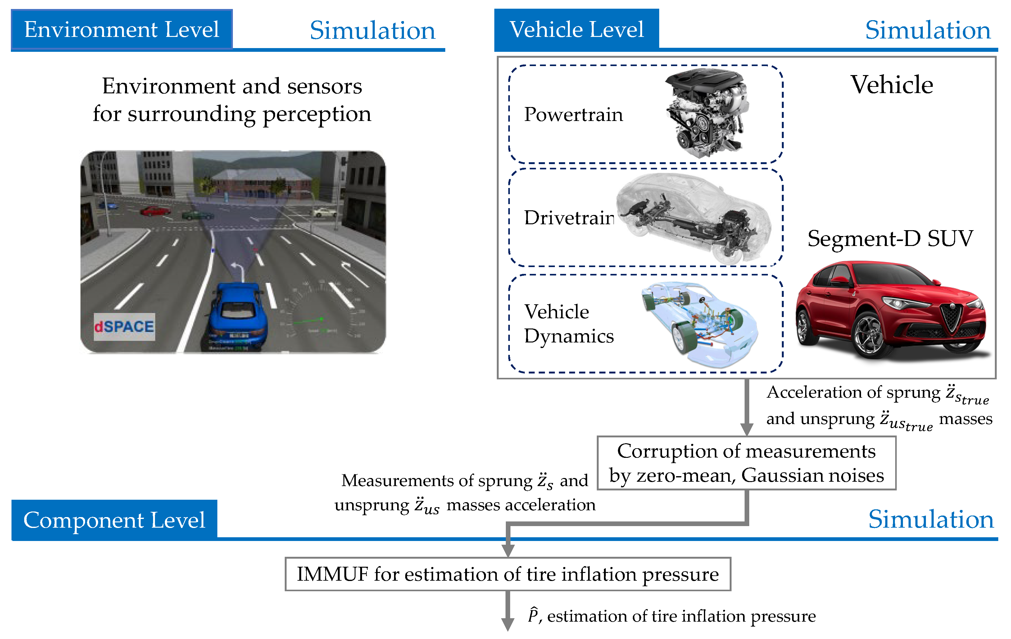
4. Tire Inflation Pressure Estimation
5. Algorithm Validation
5.1. Simulation Platform
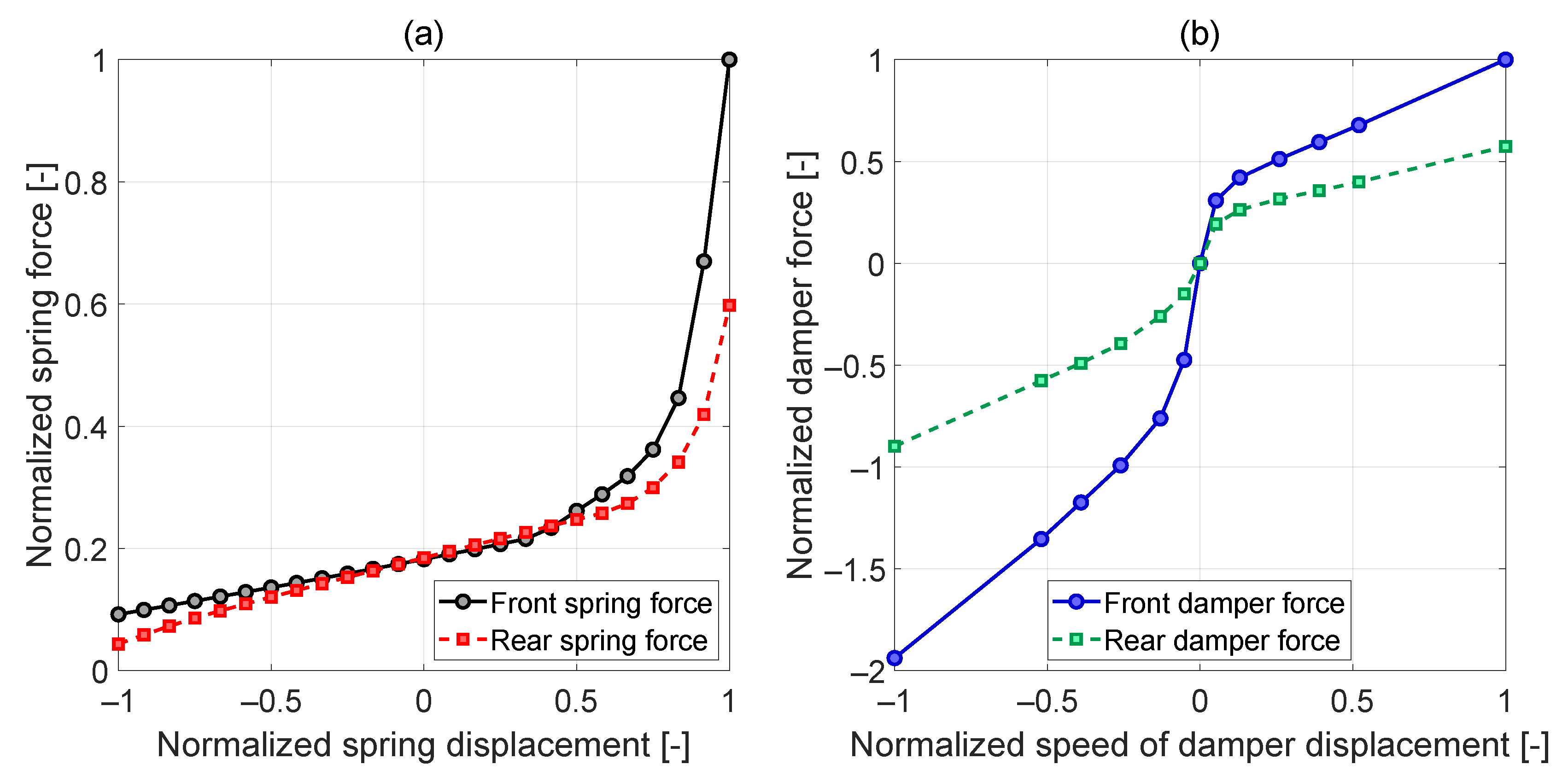
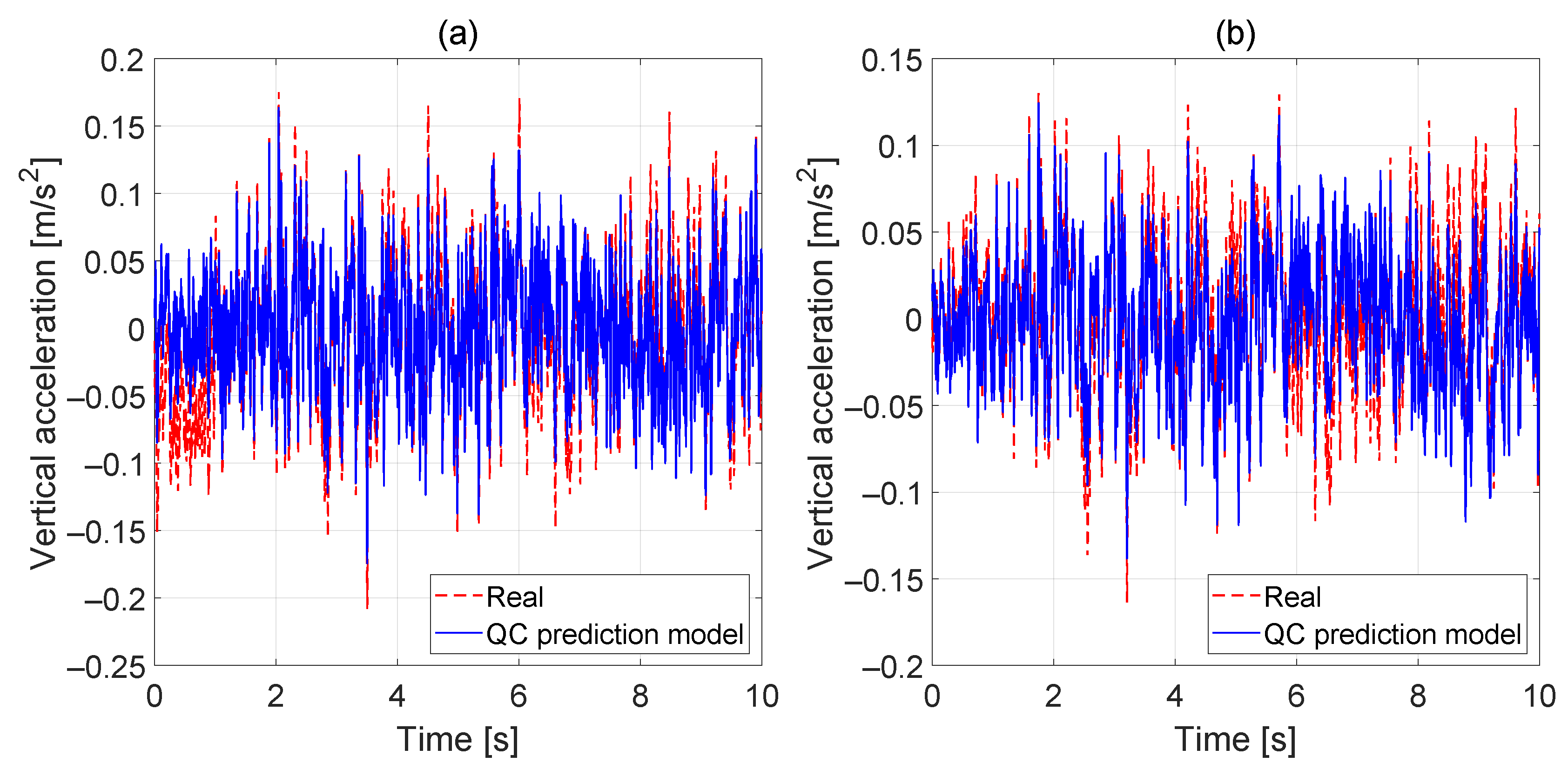
5.2. 2DOF QC Parameters Identification
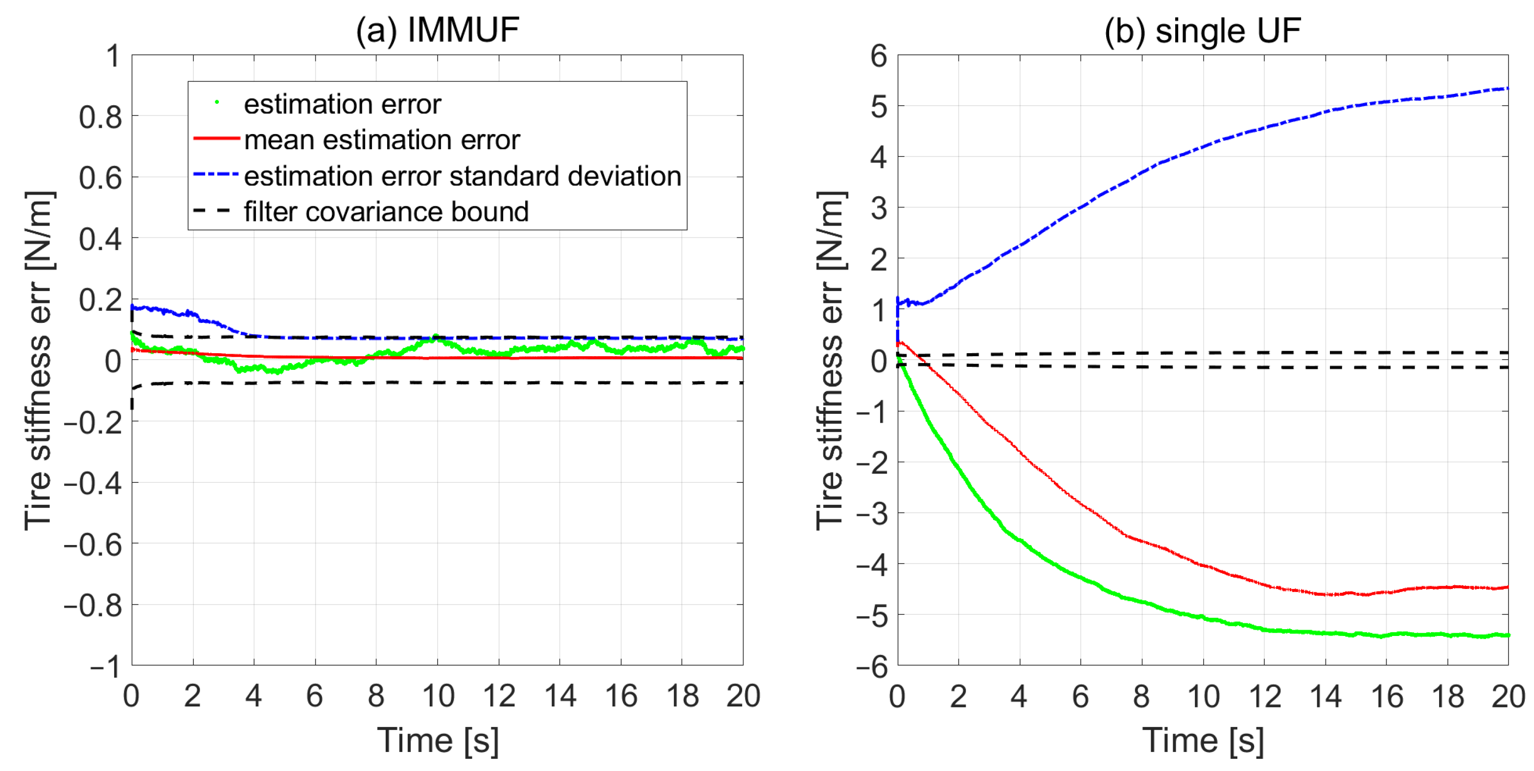
5.3. Monte Carlo Simulation
- Mean estimation error from all the Monte Carlo samples (the red line in Figure 6). For each -th time step, the mean estimation error is calculated as
- Standard deviation of the estimation errors (the dashed blue line in Figure 6). For each -th time step, the standard deviation of the errors is calculated as
- Covariance bound computed by the filter (the dashed black line in Figure 6). For each -th time step, the -bounds is calculated by the square root of the diagonal elements of the covariance matrix P, as
- Comparison of sample estimation error (the green line in Figure 6) with the -bounds.
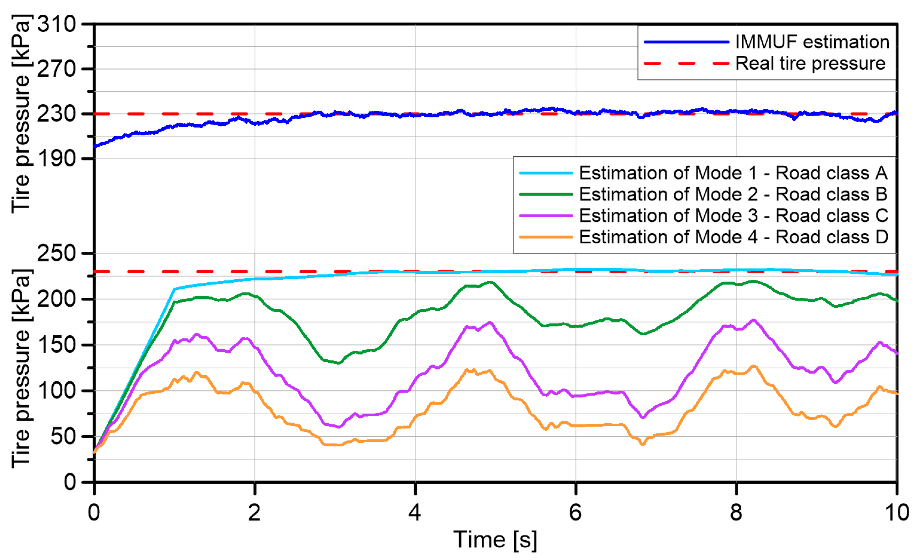
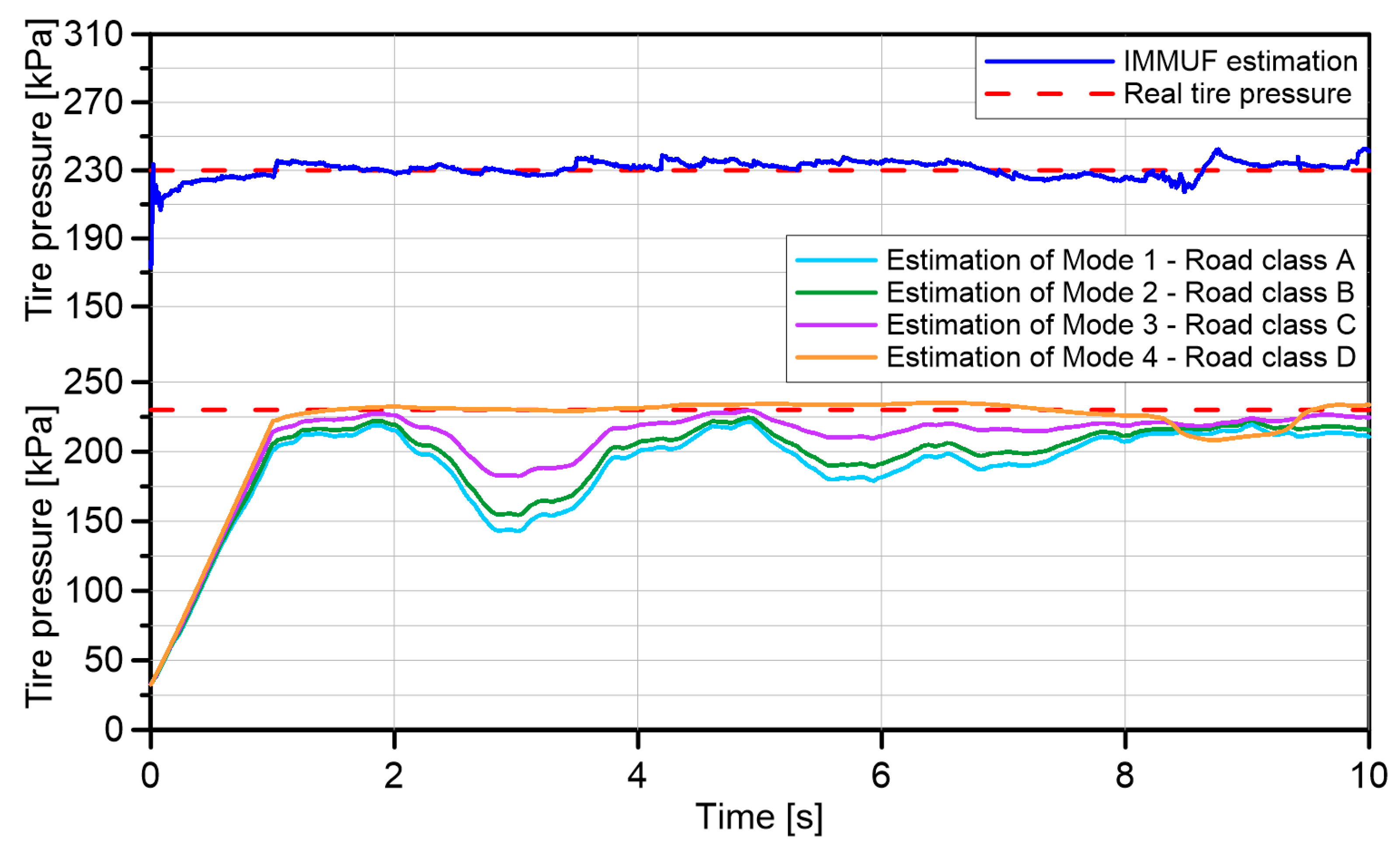
5.4. Tire Inflation Pressure Estimation
6. Conclusions
Author Contributions
Funding
Institutional Review Board Statement
Informed Consent Statement
Data Availability Statement
Conflicts of Interest
Abbreviations
| NHTSA | National Highway Traffic Safety Administration |
| TPMS | Tire Pressure Monitoring System |
| dTPMS | direct Tire Pressure Monitoring System |
| iTPMS | indirect Tire Pressure Monitoring System |
| KF | Kalman Filter |
| EKF | Extended Kalman Filter |
| UKF | Unscented Kalman Filter |
| MM | Multiple Model |
| IMM | Interactive Multiple Model |
| IMMUF | Interacting Multiple Model Unscented Filter |
| 2DOF | Two Degree Of Freedom |
| QC | Quarter Car |
| PSD | Power Spectral Density |
| MTM | Markov Transition Matrix |
| RMSE | root Mean Square Error |
| ASM | Automotive Simulation Model |
Nomenclature
| Symbol | Description | Symbol | Description |
| Sprung mass | Unsprung mass | ||
| vehicle chassis mass | loading mass | ||
| total sprung mass of the vehicle | l | wheelbase | |
| rear semiwheel base | inflation pressure increment | ||
| Linear damping coefficient | Non-linear square damping coefficient | ||
| Linear spring stiffness coefficient | Non-linear cube spring stiffness coefficient | ||
| Tire stiffness coefficient | vertical stiffness at the nominal inflation pressure | ||
| sprung mass vertical displacement | unsprung mass vertical displacement | ||
| Symbol | Description | Symbol | Description |
| road profile | nominal pressure | ||
| effective pressure | pressure effect on vertical stiffness | ||
| angular frequency | PSD | ||
| road roughness variance | v | vehicle longitudinal velocity | |
| linear shape filter parameter | probability vector | ||
| reference spacial frequency | lower spatial frequency | ||
| upper spatial frequency | Probability transition matrix | ||
| Q | process noise covariance matrix | state vector | |
| measurement vector | process function | ||
| measurement function | P | covariance matrix | |
| noise covariance matrix | sprung mass acceleration variance | ||
| time step | noise |
References
- Elfasakhany, A. Tire Pressure Checking Framework: A Review Study. Reliab. Eng. Resil. 2019, 1, 12–28. [Google Scholar]
- Mayer, A.; Emig, G.; Gmehling, B.; Popovska, N.; Hölemann, K.; Buck, A. Passive regeneration of catalyst coated Knitted fiber Diesel particulate traps. SAE Trans. 1996, 105, 36–44. [Google Scholar]
- Isermann, R. Automotive Control: Modeling and Control of Vehicles; Springer: Berlin/Heidelberg, Germany, 2022. [Google Scholar]
- Persson, N.; Gustafsson, F.; Drevö, M. Indirect tire pressure monitoring using sensor fusion. SAE Trans. 2002, 111, 1657–1662. [Google Scholar]
- Weispfenning, T. Fault detection and diagnosis of components of the vehicle vertical dynamics. Meccanica 1997, 32, 459–472. [Google Scholar] [CrossRef]
- Isermann, R.; Wesemeier, D. Indirect vehicle tire pressure monitoring with wheel and suspension sensors. IFAC Proc. Vol. 2009, 42, 917–922. [Google Scholar] [CrossRef]
- Solmaz, S. A Novel Method for Indirect Estimation of Tire Pressure. J. Dyn. Syst. Meas. Control 2016, 138, 054501. [Google Scholar] [CrossRef]
- Reina, G.; Gentile, A.; Messina, A. Tyre pressure monitoring using a dynamical model-based estimator. Veh. Syst. Dyn. 2015, 53, 568–586. [Google Scholar] [CrossRef]
- Kang, S.W.; Kim, J.S.; Kim, G.W. Road roughness estimation based on discrete Kalman filter with unknown input. Veh. Syst. Dyn. 2019, 57, 1530–1544. [Google Scholar] [CrossRef]
- Lee, D.H.; Yoon, D.S.; Kim, G.W. New indirect tire pressure monitoring system enabled by adaptive extended Kalman filtering of vehicle suspension systems. Electronics 2021, 10, 1359. [Google Scholar] [CrossRef]
- Tsunashima, H.; Murakami, M.; Miyataa, J. Vehicle and road state estimation using interacting multiple model approach. Veh. Syst. Dyn. 2006, 44, 750–758. [Google Scholar] [CrossRef]
- Battistini, S.; Brancati, R.; Lui, D.G.; Tufano, F. Enhancing ADS and ADAS Under Critical Road Conditions Through Vehicle Sideslip Angle Estimation via Unscented Kalman Filter-Based Interacting Multiple Model Approach. In Proceedings of the Advances in Italian Mechanism Science; Springer International Publishing: Cham, Switzerland, 2022; pp. 450–460. [Google Scholar]
- Ping, X.; Cheng, S.; Yue, W.; Du, Y.; Wang, X.; Li, L. Adaptive estimations of tyre–road friction coefficient and body’s sideslip angle based on strong tracking and interactive multiple model theories. Proc. Inst. Mech. Eng. Part D J. Autom. Eng. 2020, 234, 3224–3238. [Google Scholar] [CrossRef]
- Musa, A.; Pipicelli, M.; Spano, M.; Tufano, F.; De Nola, F.; Di Blasio, G.; Gimelli, A.; Misul, D.A.; Toscano, G. A review of model predictive controls applied to advanced driver-assistance systems. Energies 2021, 14, 7974. [Google Scholar] [CrossRef]
- Mohite, A.G.; Mitra, A.C. Development of linear and non-linear vehicle suspension model. Mater. Today Proc. 2018, 5, 4317–4326. [Google Scholar] [CrossRef]
- Sayers, M.W. The Little Book of Profiling: Basic Information about Measuring and Interpreting Road Profiles; Technical Report; University of Michigan, Transportation Research Institute: Ann Arbor, MI, USA, 1998. [Google Scholar]
- Hurel, J.; Mandow, A.; García-Cerezo, A. Kinematic and dynamic analysis of the McPherson suspension with a planar quarter-car model. Veh. Syst. Dyn. 2013, 51, 1422–1437. [Google Scholar] [CrossRef]
- McGee, C.G.; Haroon, M.; Adams, D.E.; Luk, Y.W. A frequency domain technique for characterizing nonlinearities in a tire-vehicle suspension system. J. Vib. Acoust. 2005, 127, 61–76. [Google Scholar] [CrossRef]
- Nagarkar, M.P.; Patil, G.J.V.; Patil, R.N.Z. Optimization of nonlinear quarter car suspension–seat–driver model. J. Adv. Res. 2016, 7, 991–1007. [Google Scholar] [CrossRef] [Green Version]
- Lemaitre, J. Handbook of Materials Behavior Models, Three-Volume Set: Nonlinear Models and Properties; Elsevier: Amsterdam, The Netherlands, 2001. [Google Scholar]
- Guiggiani, M. The Science of Vehicle Dynamics; Springer: Pisa, Italy, 2014; p. 15. [Google Scholar]
- Maher, D.; Young, P. An insight into linear quarter car model accuracy. Veh. Syst. Dyn. 2011, 49, 463–480. [Google Scholar] [CrossRef]
- Wong, J.Y. Theory of Ground Vehicles; John Wiley & Sons: Hoboken, NJ, USA, 2022. [Google Scholar]
- Taylor, R.; Bashford, L.; Schrock, M. Methods for measuring vertical tire stiffness. Trans. ASAE 2000, 43, 1415–1419. [Google Scholar] [CrossRef]
- Besselink, I.; Schmeitz, A.; Pacejka, H. An improved Magic Formula/Swift tyre model that can handle inflation pressure changes. Veh. Syst. Dyn. 2010, 48, 337–352. [Google Scholar] [CrossRef]
- ISO (International Organization for Standardization) 8608:2016; Mechanical Vibration—Road Surface PROFILES—Reporting of Measured Data. Available online: https://www.iso.org/standard/71202.html (accessed on 18 October 2022).
- Ulsoy, A.G.; Peng, H.; Çakmakci, M. Automotive Control Systems; Cambridge University Press: Cambridge, UK, 2012. [Google Scholar]
- Tyan, F.; Hong, Y.F.; Tu, S.H.; Jeng, W.S. Generation of random road profiles. J. Adv. Eng. 2009, 4, 1373–1378. [Google Scholar]
- Dharankar, C.S.; Hada, M.K.; Chandel, S. Numerical generation of road profile through spectral description for simulation of vehicle suspension. J. Braz. Soc. Mech. Sci. Eng. 2017, 39, 1957–1967. [Google Scholar] [CrossRef]
- Schiehlen, W. White noise excitation of road vehicle structures. Sadhana 2006, 31, 487–503. [Google Scholar] [CrossRef] [Green Version]
- Goenaga, B.; Fuentes, L.; Mora, O. Evaluation of the methodologies used to generate random pavement profiles based on the power spectral density: An approach based on the International Roughness Index. Ing. E Investig. 2017, 37, 49–57. [Google Scholar] [CrossRef] [Green Version]
- Shannon, C.E. Communication in the presence of noise. Proc. IRE 1949, 37, 10–21. [Google Scholar] [CrossRef]
- Lenkutis, T.; Čerškus, A.; Šešok, N.; Dzedzickis, A.; Bučinskas, V. Road surface profile synthesis: Assessment of suitability for simulation. Symmetry 2020, 13, 68. [Google Scholar] [CrossRef]
- Battistini, S.; Menegaz, H.M. Interacting multiple model unscented filter for tracking a ballistic missile during its boost phase. In Proceedings of the 2017 IEEE Aerospace Conference, Big Sky, MT, USA, 4–11 March 2017; pp. 1–8. [Google Scholar]
- Varshney, D.; Bhushan, M.; Patwardhan, S.C. State and parameter estimation using extended Kitanidis Kalman filter. J. Process Control 2019, 76, 98–111. [Google Scholar] [CrossRef]
- Stellantis. Segment-D SUV Vehicle Specifications’ Documents. 2022. Available online: https://stellantis-na-product-media.info/alfa-romeo/stelvio (accessed on 29 November 2022).
- Maino, C.; Misul, D.; Musa, A.; Spessa, E. Optimal mesh discretization of the dynamic programming for hybrid electric vehicles. Appl. Energy 2021, 292, 116920. [Google Scholar] [CrossRef]
- Gimelli, A.; Luongo, A.; Muccillo, M. Efficiency and cost optimization of a regenerative Organic Rankine Cycle power plant through the multi-objective approach. Appl. Therm. Eng. 2017, 114, 601–610. [Google Scholar] [CrossRef]
- Brancati, R.; Muccillo, M.; Tufano, F. Crank mechanism friction modeling for control-oriented applications. In Proceedings of the The International Conference of IFToMM ITALY; Springer: Cham, Switzerland, 2020; pp. 729–737. [Google Scholar]
- Petrillo, A.; Prati, M.V.; Santini, S.; Tufano, F. Improving the NOx reduction performance of an Euro VI d SCR System in real-world condition via nonlinear model predictive control. Int. J. Engine Res. 2021. [CrossRef]
- Papadopoulos, C.E.; Yeung, H. Uncertainty estimation and Monte Carlo simulation method. Flow Meas. Instrum. 2001, 12, 291–298. [Google Scholar] [CrossRef]
- De Nola, F.; Giardiello, G.; Noviello, B.; Tufano, F. A control-oriented and physics-based model of the engine crank mechanism friction for the base calibration: Parametric analysis. In Proceedings of the AIP Conference Proceedings; AIP Publishing LLC: College Park, MD, USA, 2019; Volume 2191, p. 020060. [Google Scholar]
- Harding, B.; Tremblay, C.; Cousineau, D. Standard errors: A review and evaluation of standard error estimators using Monte Carlo simulations. Quant. Methods Psychol. 2014, 10, 107–123. [Google Scholar] [CrossRef]
- Harrison, R.L. Introduction to monte carlo simulation. In Proceedings of the AIP Conference Proceedings; American Institute of Physics: College Park, MD, USA, 2010; Volume 1204, pp. 17–21. [Google Scholar]
- Ge, Q.; Shao, T.; Duan, Z.; Wen, C. Performance analysis of the Kalman filter with mismatched noise covariances. IEEE Trans. Autom. Control 2016, 61, 4014–4019. [Google Scholar] [CrossRef]
- Šroubek, F.; Šorel, M.; Žák, J. Precise international roughness index calculation. Int. J. Pavement Res. Technol. 2022, 15, 1413–1419. [Google Scholar] [CrossRef]


| Quantity | Value | Quantity | Value |
|---|---|---|---|
| Mass of vehicle chassis (vehicle body) | 1788 kg | Height of the center of mass | 0.6 m |
| Front semi-wheelbase | 1.347 m | Rear semi-wheelbase | 1.471 m |
| Front track width | 1.606 m | Rear track width | 1.6364 m |
| Yaw moment of inertia | 3230 kg m2 | Frontal area | 2.75 m2 |
| Front wheel mass | 61.14 kg | Rear wheel mass | 52.75 kg |
| Nominal pressure of inflated tire | 250 kPa | vertical stiffness at | 264,700 N/m |
| Parameter | Description |
|---|---|
| Linear damping coefficient | |
| Non-linear square damping coefficient | |
| Linear spring stiffness coefficient | |
| Non-linear cube spring stiffness coefficient |
| Parameter | Road Class A | Road Class B | Road Class C | Road Class D |
|---|---|---|---|---|
| [Ns/m] | 6576 | 4585 | 14,819 | 14,708 |
| [Ns/m2] | 4319 | 6016 | 5839 | 4555 |
| [N/m] | 113,086 | 173,415 | 94,544 | 118,114 |
| [N/m3] | 130,098 | 151,886 | 62,836 | 121,723 |
| Parameter | Range |
|---|---|
| (130–230) [kPa] | |
| v | 40–80 [km/h] |
| a | 0–3 [-] |
Publisher’s Note: MDPI stays neutral with regard to jurisdictional claims in published maps and institutional affiliations. |
© 2022 by the authors. Licensee MDPI, Basel, Switzerland. This article is an open access article distributed under the terms and conditions of the Creative Commons Attribution (CC BY) license (https://creativecommons.org/licenses/by/4.0/).
Share and Cite
Brancati, R.; Tufano, F. Indirect Estimation of Tire Pressure on Several Road Pavements via Interacting Multiple Model Approach. Machines 2022, 10, 1221. https://doi.org/10.3390/machines10121221
Brancati R, Tufano F. Indirect Estimation of Tire Pressure on Several Road Pavements via Interacting Multiple Model Approach. Machines. 2022; 10(12):1221. https://doi.org/10.3390/machines10121221
Chicago/Turabian StyleBrancati, Renato, and Francesco Tufano. 2022. "Indirect Estimation of Tire Pressure on Several Road Pavements via Interacting Multiple Model Approach" Machines 10, no. 12: 1221. https://doi.org/10.3390/machines10121221