Binary Feature Description of 3D Point Cloud Based on Retina-like Sampling on Projection Planes

Abstract

A binary feature description and registration algorithm for a 3D point cloud based on retina-like sampling on projection planes (RSPP) are proposed in this paper. The algorithm first projects the point cloud within the support radius around the key point to the XY, YZ, and XZ planes of the Local Reference Frame (LRF) and performs retina-like sampling on the projection plane. Then, the binarized Gaussian density weight values at the sampling points are calculated and encoded to obtain the RSPP descriptor. Finally, rough registration of point clouds is performed based on the RSPP descriptor, and the RANSAC algorithm is used to optimize the registration results. The performance of the proposed algorithm is tested on public point cloud datasets. The test results show that the RSPP-based point cloud registration algorithm has a good registration effect under no noise, 0.25 mr, and 0.5 mr Gaussian noise. The experimental results verify the correctness and robustness of the proposed registration method, which can provide theoretical and technical support for the 3D point cloud registration application.

1. Introduction

In recent years, with the rapid development of three-dimensional (3D) point cloud sensor hardware, point cloud data has been widely used in unmanned driving [1], intelligent robot [2], surveying and mapping [3], remote sensing [4], and virtual reality [5]. Point cloud registration is a fundamental problem in 3D computer vision and photogrammetry. Given two groups of point clouds with overlapping information, the aim of registration is to find the transformation that best aligns the two groups of point clouds to the same coordinate system [6,7]. Point cloud registration plays a significant role in the above point cloud applications. Point cloud registration is generally achieved by matching point cloud feature descriptors. Although significant progress has been made in point cloud feature description and registration, several problems, such as sensitivity to noise [8] and large storage memory [9], still require further study. The measured point cloud usually contains much noise, and the memory of the mobile hardware platform is often limited. Therefore, it is urgent to develop a point cloud feature description and registration algorithm that is robust to noise and occupies less memory, which is of great significance to the practical application of the point cloud registration algorithm. Retina-like sampling has been successfully applied in the field of image registration, reducing the impact of the image registration algorithm on noise and improving image registration accuracy [10]. Inspired by this, this paper attempts to explore whether the retina-like sampling can improve point cloud registration accuracy. Binary feature descriptors have less memory than floating-point feature descriptors [11]. Therefore, to reduce the sensitivity of the cloud registration algorithm to noise, reduce descriptor storage memory and improve algorithm accuracy, combining the retina-like sampling technology and binary feature idea, this paper proposes a binary feature description and registration method based on retina-like sampling on projection planes according to the structural characteristics of the common 3D point cloud.

The main contributions of this paper are as follows:

1. A binary feature description method for 3D point cloud based on retina-like sampling on projection planes (RSPP) is proposed, and Gaussian kernel function is introduced to reduce the sensitivity of the feature descriptor to noise;

2. A point cloud registration method based on RSPP is proposed, and the accuracy of the registration algorithm is verified on commonly used 3D point cloud datasets.

2. Related Work

Up to now, scholars have proposed many point cloud local feature description methods. This section mainly reviews some well-known 3D point cloud feature description methods. Spin Images (SI) [12] is one of the most popular feature descriptors in the early stage. SI forms its descriptor by accumulating the number of adjacent points into a two-dimensional histogram. However, the descriptiveness of SI is relatively low and easily affected by the mesh resolution (mr) of the point cloud. Therefore, to improve the descriptiveness, 3D Shape Context (3DSC) [13] expands the 2D shape context to the 3D shape context and accumulates the number of weighted points into 3D spatial point density according to spatial division. Point Feature Histogram (PFH) [8] encodes the angle between point pairs formed by the combination of all adjacent points in the local surface support domain and the surface normal, but PFH has high computational complexity and poor real-time performance. To improve the calculation efficiency, Fast Point Feature Histogram (FPFH) [14] calculates the Simplified Point Feature Histograms (SPFH) of all points in the local surface support domain and assigns different weights to form the final descriptor. Signature of Histograms of OrienTations (SHOT) [15] first establishes a Local Reference Frame (LRF) at key points and then divides the local sphere into a group subspace along the radial, azimuth, and elevation axes. The local 3D surface is described by coding the normal histogram of adjacent points in the LRF coordinate system. Rotational Projection Statistics (ROPS) [16] rotates and projects the point cloud onto a two-dimensional (2D) plane, computes distribution statistics of these projection points, including the low-order central moment and entropy, and finally combines these distribution statistics into the feature histogram. Signature of Geometric Centroids (SGC) [17] establishes an LRF for key points, divides the voxel grid along the three axes of the LRF, counts the number of points in each voxel grid, and calculates the center of gravity of the points. Descriptors of SGC will be generated by combining the number of points and the center of gravity of each voxel. 3DHOPD [18] uses the location of key points and the one-dimensional Histogram of Point Distributions (HOPD) along each axis of the LRF as a feature description. Triple Orthogonal Local Depth Images(TOLDI) [19] firstly projects the local point cloud around the key point to the XY, YZ, and XZ planes of the LRF coordinate system. Then, each plane is evenly divided into grids, and the value at the grid is the minimum projection distance between the projected points and the plane. Finally, the values of all grids are concatenated into a descriptor. Binary Shape Context (BSC) [20] is a robust and descriptive 3D binary shape context descriptor. Based on the TOLDI, the Gaussian weighted projection point distance feature and the Gaussian weighted projection point density feature are comprehensively considered and binarized, respectively, and finally are spliced into a BSC descriptor. Weighted Height Image (WHI) [21] encodes local point cloud distance features by introducing a custom weighting function. Rotational Contour Signatures (RCS) [22] describe 2D contour information derived from 3D to 2D projection of local surfaces. Local Voxelized Structure (LoVS) [11] generates a string of binary feature descriptors according to whether the local voxel structure around the feature points contains points. On this basis, multi-scale Local Voxelized Structure (mLoVS) [23] makes up for the limitations of LoVS on scale variation. Further based on LoVS features, Voxel-based Buffer-weighted Binary Descriptor (VBBD) [24] enhances the robustness of feature descriptors to boundary effects and density variations by introducing a Gaussian kernel function. Divisional Local Feature Statistics(DLFS) [25] divides a local space into several partitions along the projected radial direction and then performs statistics of one spatial and three geometric properties for each partition. Local Angle Statistics Histogram (LASH) [26] forms a description of local shape geometry by encoding its attribute as the angle between the normal vector of the point and the vector formed by the point and other points in its local neighborhood. Kernel Density Descriptor (KDD) [27] encodes information about the entire 3D space around feature points through kernel density estimation. Grid Normals Deviation Angles Statistics (GNDAS) [28] firstly divides the local surface into several grids evenly along the x-axis and y-axis of the LRF and then counts the deviation angle of the normal at grid points.

3. Binary Feature of Retina-like Sampling on Projection Planes

The binary feature description process of retina-like sampling on the projection planes is shown in Figure 1. Firstly, the key points are detected from the input point cloud. Secondly, the LRF is constructed at key points. Then, all points within the support radius are projected onto the XY, YZ, and XZ planes, retina-like sampling is performed on the projection planes, and the Gaussian density weight values at the sampling points are calculated. Finally, the weight values are binarized and encoded to form the RSPP feature descriptor.

3.1. Key Points Detection

Key point detection is a basic and important step in point cloud registration. A key point detector has at least two requirements: high repeatability and good discrimination. At present, the widely used key point detectors include Harris 3D [29], 3D SURF [30], NARF [31], ISS [32], etc. Due to the good repeatability and high computational efficiency of the ISS key point detector [17], this paper selects the ISS key point detector. The specific process of ISS is as follows:

(1) Assuming $\mathbf{P}$ is the input point cloud, an LRF is established for each point ${\mathbf{p}}_i$, and a search radius $r_{search}$ is set for all points;

(2) Determine all points in the area with ${\mathbf{p}}_i$ as the center and $r_{search}$ as the search radius, and calculate the weight $w_{ij}$ of these points, whose expression is as follows:

$$\begin{array}{cc}{w}_{ij}=\frac{1}{\Vert {\mathbf{p}}_i-{\mathbf{p}}_j\Vert },& \Vert {\mathbf{p}}_i-{\mathbf{p}}_j\Vert <r_{search}\end{array},$$

(1)

(3) Establish the covariance matrix $\mathrm{cov}\left({\mathbf{p}}_i\right)$ of ${\mathbf{p}}_i$:

$$\mathrm{cov}\left({\mathbf{p}}_i\right)={\displaystyle \sum _{\Vert {\mathbf{p}}_i-{\mathbf{p}}_j\Vert <r_{search}}{w}_{ij}\left({\mathbf{p}}_i-{\mathbf{p}}_j\right){\left({\mathbf{p}}_i-{\mathbf{p}}_j\right)}^T}/{\displaystyle \sum _{\Vert {\mathbf{p}}_i-{\mathbf{p}}_j\Vert <r_{search}}{w}_{ij}},$$

(2)

(4) The eigenvalues of covariance matrix $\mathrm{cov}\left({\mathbf{p}}_i\right)$ are solved and arranged as $\left\{{\lambda }_i^1,{\lambda }_i^2,{\lambda }_i^3\right\}$ from large to small,

(5) Set the thresholds ${\epsilon }_1$ and ${\epsilon }_2$, and select the ${\mathbf{p}}_i$ point satisfying ${\lambda }_i^2/{\lambda }_i^1<{\epsilon }_1$ and ${\lambda }_i^3/{\lambda }_i^2<{\epsilon }_2$ as the key point

3.2. LRF Construction

A unique and stable LRF plays an essential role in the accuracy and stability of feature matching. Suppose ${\mathbf{p}}_i$ is a key point in the input point cloud $\mathbf{P}$, and the point set in the sphere with ${\mathbf{p}}_i$ as the center and radius $r_{LRF}$ is defined as ${\mathbf{Q}}_i=\left\{{\mathbf{q}}_{ij},\Vert {\mathbf{q}}_{ij}-{\mathbf{p}}_i\Vert <r_{LRF}\right\}$, where ${\mathbf{q}}_{ij}$ is other points around ${\mathbf{p}}_i$, and $\Vert {\mathbf{q}}_{ij}-{\mathbf{p}}_i\Vert$ is the Euclidean distance between ${\mathbf{q}}_{ij}$ and ${\mathbf{p}}_i$. Similar to reference [15], the distance weight covariance matrix $Cov$ of feature points and neighborhood points are used to construct the LRF, and the matrix $Cov$ is defined as follows:

$$Cov=\frac{1}{{\displaystyle \sum w_{ij}}}{\displaystyle \sum _{{\mathbf{q}}_{ij}\in {\mathbf{Q}}_i}{w}_{ij}\left({\mathbf{q}}_{ij}-{\mathbf{p}}_i\right){\left({\mathbf{q}}_{ij}-{\mathbf{p}}_i\right)}^T},$$

(3)

$$w_{ij}=R-\Vert {\mathbf{q}}_{ij}-{\mathbf{p}}_i\Vert ,$$

(4)

The eigenvalue decomposition is performed on matrix $Cov$. The eigenvector corresponding to the minimum eigenvalue is the normal vector $\mathbf{n}\left({\mathbf{p}}_i\right)$ at the key point, and the eigenvector corresponding to the maximum eigenvalue is the candidate X-axis direction ${\mathbf{X}}_{cand}$ of the LRF. Since the direction of the feature vector has symbol uncertainty, the symbol ambiguity is eliminated by the following methods:

$$\mathbf{Z}\left({\mathbf{p}}_i\right)=\{\begin{array}{cc}\mathbf{n}\left({\mathbf{p}}_i\right)& \begin{array}{cc}if& \mathbf{n}\left({\mathbf{p}}_i\right)\cdot {\displaystyle \sum _{q_{ij}\in {\mathbf{Q}}_i}-\left({\mathbf{q}}_{ij}-{\mathbf{p}}_i\right)\ge 0}\end{array}\\ -\mathbf{n}\left({\mathbf{p}}_i\right)& else\end{array},$$

(5)

$$\mathbf{X}\left({\mathbf{p}}_i\right)=\{\begin{array}{cc}{\mathbf{X}}_{cand}& \begin{array}{cc}if& {\mathbf{X}}_{cand}\cdot {\displaystyle \sum _{{\mathbf{q}}_{ij}\in {\mathbf{Q}}_i}{w}_{ij}\left\{\left({\mathbf{q}}_{ij}-{\mathbf{p}}_i\right)-\left[\left({\mathbf{q}}_{ij}-{\mathbf{p}}_i\right)\cdot \mathbf{Z}\left({\mathbf{p}}_i\right)\right]\cdot \mathbf{Z}\left({\mathbf{p}}_i\right)\right\}\ge 0}\end{array}\\ -{\mathbf{X}}_{cand}& else\end{array},$$

(6)

Then, the constructed LRF is:

$$\mathbf{L}\left({\mathbf{p}}_i\right)=\left\{\mathbf{X}\left({\mathbf{p}}_i\right),\mathbf{Z}\left({\mathbf{p}}_i\right)\times \mathbf{X}\left({\mathbf{p}}_i\right),\mathbf{Z}\left({\mathbf{p}}_i\right)\right\},$$

(7)

3.3. RSPP Descriptor

Some studies have shown that retina-like sampling has many successful cases in image feature matching, such as BRISK [33], FREAK [10], and DAISY [34]. These cases show that retina-like sampling can improve the accuracy of image registration. The original intention of this paper is to apply the idea of retina-like sampling to point cloud registration and explore its potential in improving the accuracy of point cloud registration. Therefore, a point cloud feature extraction method based on retina-like sampling on the projection plane is proposed in this paper, as shown in Figure 2. Firstly, all local points within a sphere of radius $R$ centered on the key point are acquired in 3D space, as shown in Figure 2a. Secondly, the local point cloud is projected onto the $XY$, $YZ$, and $XZ$ planes of the LRF, and the retina-like sampling points centered on the key point are established on each projection plane, as shown in Figure 2b. Then, we calculate and accumulate the Gaussian density weights of all points within the sampling radius to the feature sampling point, binarize the weight sum according to whether it is greater than the weight threshold and arrange the binarized weight sum of all feature sampling points in a fixed order to form a sub binary feature histogram, as shown in Figure 2c. Finally, the sub binary feature histograms of different projection planes are merged into the fused feature histogram, as shown in Figure 2d.

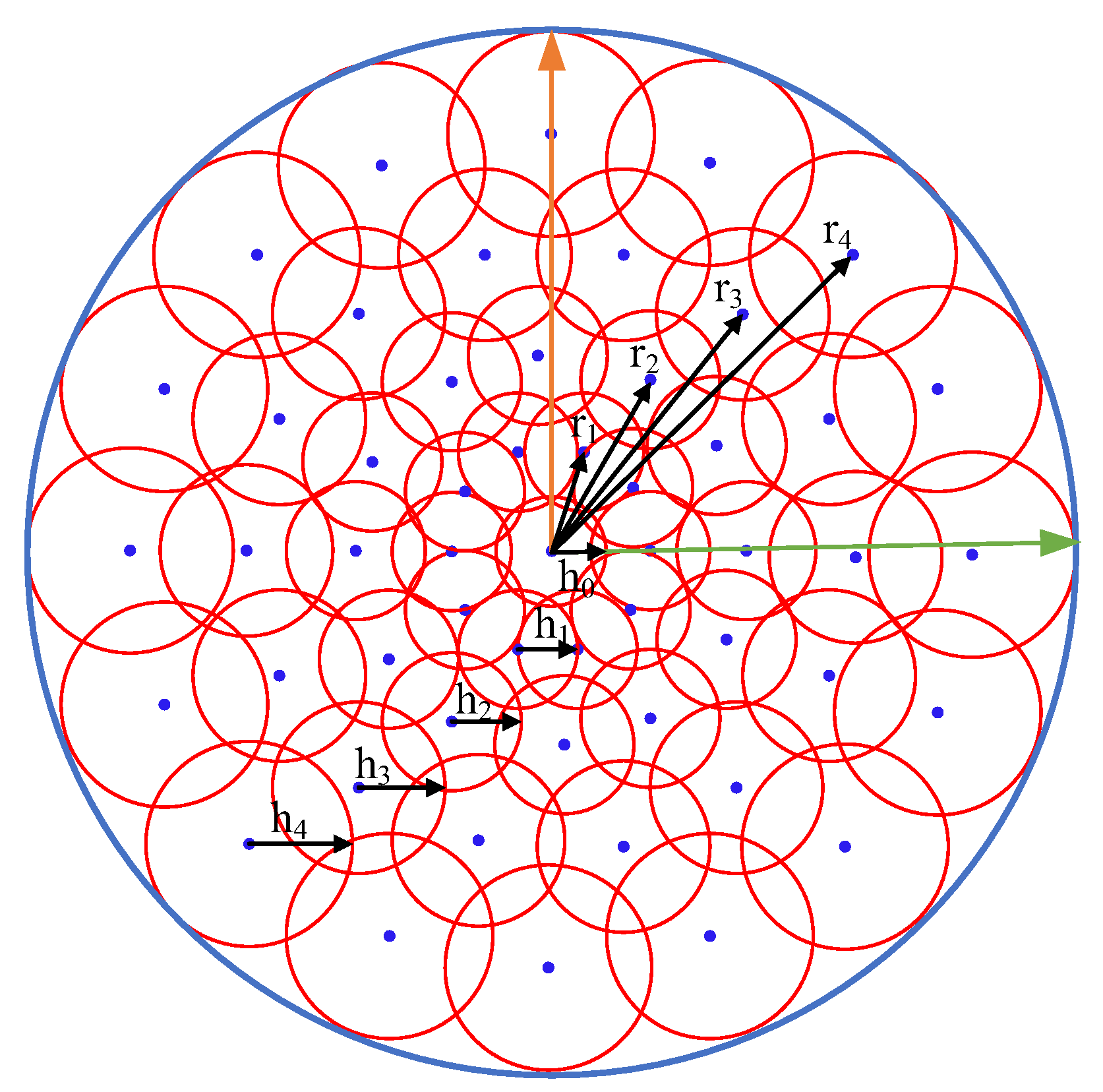
The schematic diagram of the retina-like sampling mode designed in this paper is shown in Figure 3.

In Figure 3, the blue dot represents the sampling point, the red circle represents the sampling area, the radius of the sampling circle of the same layer is the same, and the radius from the inside to the outside is $h_0,h_1,\dots ,h_n$; the distance between the center of the sampling circle of the same layer and the origin of the local coordinate system is the same, and the distance from the inside to the outside is $r_1,\dots ,r_n$; $n$ is the number of layers of the sampling circle; The number of sampling circles in each layer is $N_0,N_1,\dots ,N_n$ and $N_0=1$.

It is assumed that for a specific sampling point ${\mathbf{p}}_{si}$, the point set in the circle with the sampling radius of $h_s$ is defined as ${\mathbf{C}}_{si}=\left\{{\mathbf{q}}_{sij},\Vert {\mathbf{q}}_{sij}-{\mathbf{p}}_{si}\Vert <h_s\right\}$. It is believed that each point in the sampling area impacts the feature description of the sampling point ${\mathbf{p}}_{si}$. The impact is represented by the sum of Gaussian density weights in this paper, as shown in the following formula:

$$\begin{array}{cc}{w}_{si}={\displaystyle \sum _{n=1}^{m_{si}}\frac{1}{\sqrt{2\pi {\sigma }_s}}{e}^{-\frac{{\Vert {\mathbf{q}}_{sij}-{\mathbf{p}}_{si}\Vert }^2}{2{\sigma }_s^2}}},& {\mathbf{q}}_{sij}\in {\mathbf{C}}_{si}\end{array},$$

(8)

where ${\sigma }_s$ represents the sampling standard deviation, let ${\sigma }_s=h_s/3$ in this paper, and $m_{si}$ represents the number of points in the sampling area.

In order to enhance the robustness of feature description and improve the speed of feature matching, the weight sum is binarized, as shown in the following formula:

$$w_{si}=\{\begin{array}{cc}1& w_{si}\ge w_{thread}\\ 0& else\end{array},$$

(9)

The binary Gaussian density weight sum of the sampling points in each projection plane is arranged in a clockwise order from the inside out to obtain three sub binary histograms, and the three sub binary histograms are spliced to form a fused feature histogram.

3.4. Feature Matching

Suppose ${\mathbf{P}}^s$ and ${\mathbf{P}}^t$ represent the source point cloud and the target point cloud, respectively, their corresponding key point sets are $\left\{{\mathbf{P}}_1^s,{\mathbf{P}}_2^s,\cdots ,{\mathbf{P}}_n^s\right\}$ and $\left\{{\mathbf{P}}_1^t,{\mathbf{P}}_2^t,\cdots ,{\mathbf{P}}_m^t\right\}$, and the corresponding feature descriptors of the key point sets are $\left\{{\mathbf{f}}_1^s,{\mathbf{f}}_2^s,\cdots ,{\mathbf{f}}_n^s\right\}$ and $\left\{{\mathbf{f}}_1^t,{\mathbf{f}}_2^t,\cdots ,{\mathbf{f}}_m^t\right\}$. In order to register the source point cloud and the target point cloud, the Hamming distance is used to describe the similarity between the two descriptors. Find the nearest feature descriptor through the following formula for the descriptor ${\mathbf{f}}_i^s$ of a key point in the source point cloud.

$${\mathbf{f}}_j^t=\arg \underset{j=1,2,\dots ,m}{\min }\left(H\left({\mathbf{f}}_j^t,{\mathbf{f}}_i^s\right)\right),$$

(10)

where $H(\cdot )$ represents the Hamming distance.

The corresponding matching key point pair $\langle {\mathbf{P}}_i^s,{\mathbf{P}}_j^t\rangle$ can be obtained through the descriptor matching point pair $\langle {\mathbf{f}}_i^s,{\mathbf{f}}_j^t\rangle$. Since there will inevitably be mismatches in the registered key point pairs, to improve the registration accuracy, the Hamming distances of the descriptor matching pairs of all key points are sorted increasingly, and the smallest K-pairs of matching pairs are selected as the input of RANSAC to estimate the transformation matrix between two clouds finally.

4. Experimental Verification

4.1. Point Cloud Dataset

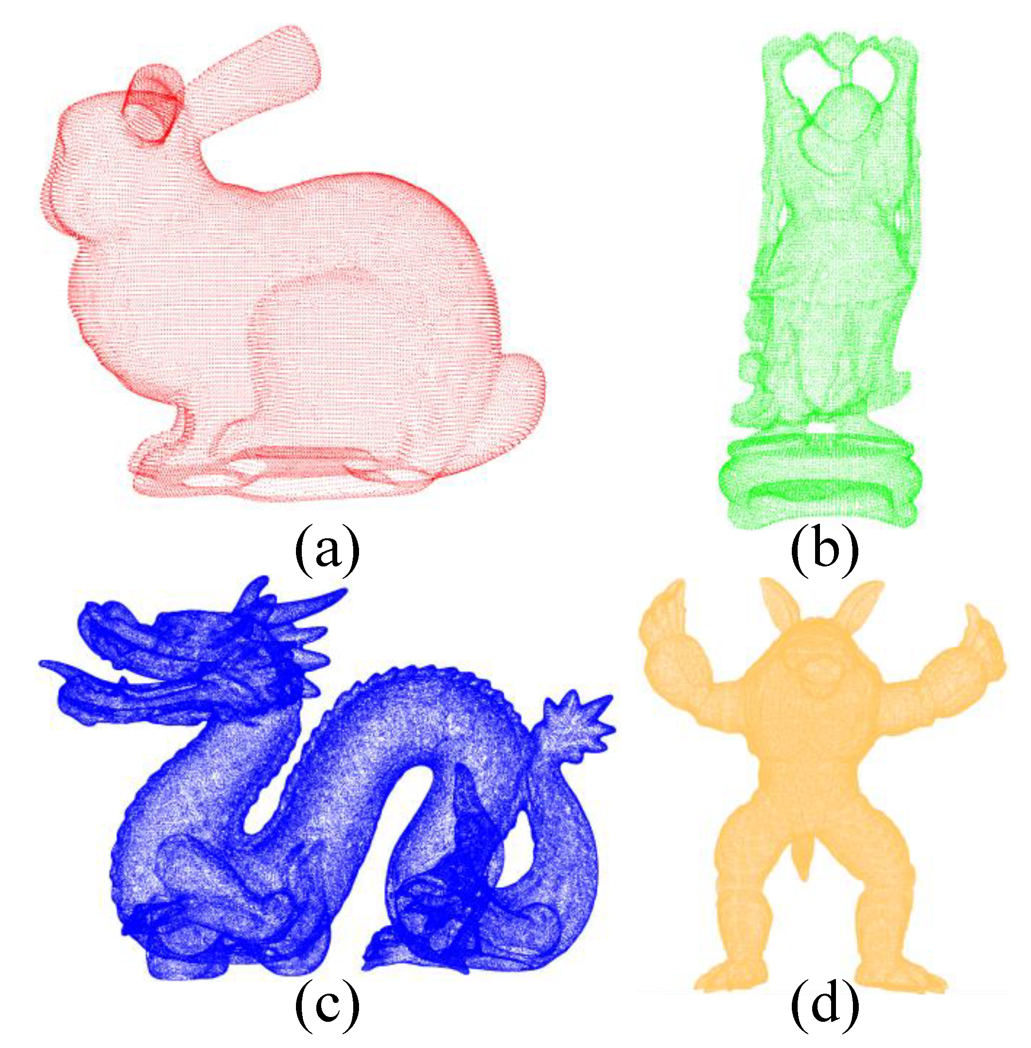
In order to prove the feasibility of the point cloud feature description and matching method based on retina-like sampling proposed in this paper, the commonly used Stanford 3D Scanning Repository [35,36,37,38] is selected as the input point cloud for algorithm verification. Most Stanford models in the Stanford 3D Scanning Repository are scanned with a Cyberware 3030 MS scanner. The Stanford models used in this paper include Stanford Bunny, Happy Buddha, Dragon, and Armadillo, as shown in Figure 4.

4.2. Evaluation Criteria

Recall vs. 1—Precision Curve (RP Curve) is widely used to evaluate the performance of point cloud feature descriptors [11,15,16]. Therefore, to quantitatively evaluate the performance of the proposed RSPP feature description and matching method, the RP curve is also adopted in this paper.

Given a source point cloud, a target point cloud, and their transformation relationship, match the descriptors of the source point cloud with the descriptors of the target point cloud and find the target point closest to the source point according to the distance of feature descriptors. If the ratio of the minimum distance to the second minimum distance is less than the threshold, the source point is considered to match the closest target point cloud. Moreover, only when the actual distance between the two points is small enough is the matching considered a true positive. Otherwise, it is considered a false positive. The specific calculation method of $1-\mathrm{Precision}$ and $\mathrm{Recall}$ is as follows. The $\mathrm{Precision}$ is the number of correct matching descriptors divided by the total number of descriptor matching, then $1-\mathrm{Precision}$ is the number of false matching descriptors divided by the total number of descriptor matching. The $\mathrm{Recall}$ is the number of correct matching descriptors divided by the number of corresponding features.

$$1-\mathrm{Precision}=\frac{\mathrm{No}.\mathrm{of}\mathrm{false}\mathrm{matches}}{\mathrm{No}.\mathrm{of}\mathrm{matches}},$$

(11)

$$\mathrm{Recall}=\frac{\mathrm{No}.\mathrm{of}\mathrm{correct}\mathrm{matches}}{\mathrm{No}.\mathrm{of}\mathrm{corresponding}\mathrm{features}},$$

(12)

where $\mathrm{No}.\mathrm{of}$ represents “the number of”.

At the same time, to quantitatively evaluate the registration algorithm’s accuracy, the registration accuracy index is used and defined as follows:

$$\mathrm{Accuracy}=\frac{\mathrm{No}.\mathrm{of}\mathrm{correct}\mathrm{matches}}{\mathrm{No}.\mathrm{of}\mathrm{total}\mathrm{matches}},$$

(13)

In order to evaluate whether a pair of registration points $\left\{{\mathbf{p}}_i,{\mathbf{p}}_j\right\}$ is correct, the root mean square error of the distance between the two coordinate positions $d_{rmse}$ is used as a criterion. If $d_{rmse}$ is less than the distance threshold ${\epsilon }_{rmse}$, it is a correct match; Otherwise, it is a wrong match. The $d_{rmse}$ is defined as follows:

$$d_{rmse}=\Vert {\mathbf{p}}_j-{\mathbf{T}}_{i2j}{\mathbf{p}}_i\Vert ,$$

(14)

where ${\mathbf{T}}_{i2j}$ represents the real coordinate transformation matrix between two clouds.

To sum up, the evaluation indicators used in this paper include the RP curve and accuracy. The larger the area under the RP curve and the higher the accuracy, indicating that the better the registration result is, the better the point cloud registration algorithm’s performance.

4.3. Parameter Analysis

It can be seen from the above that the variable parameters involved in the calculation process of the binary feature based on retina-like sampling on the projection planes include the support radius $R$, the number of sampling layers $n$, the number of sampling circles per layer $N_0,N_1,\dots ,N_n$, the radius of the sampling circle $h_0,h_1,\dots ,h_n$, and the distance $r_0,r_1,\dots ,r_n$ between the center of the sampling circle and the origin of the LRF.

For the convenience of expression, let

$$\{\begin{array}{l}{h}_i={\left(k_h\right)}^n\times h_0\\ r_i=k_r^i\times h_0\end{array},$$

(15)

where $k_h$ represents the radius coefficient of the sampling circle, and $k_r^i$ represents the distance coefficient of the center of the sampling circle.

The parameter combination of the RSPP feature descriptor will significantly affect the performance of the descriptor. For example, when the support radius is large, but the number of sampling circles per layer is small, the performance of the descriptor will be poor. When the support radius is large and the number of sampling circles per layer is also large, the noise will seriously interfere with the performance of the descriptor. Therefore, finding an optimal combination of parameters is necessary to improve the performance of descriptors. To obtain the best parameter combination, take dragon data as an example to analyze the performance of the RSPP feature descriptor under different parameter combinations.

(1) 

Support radius

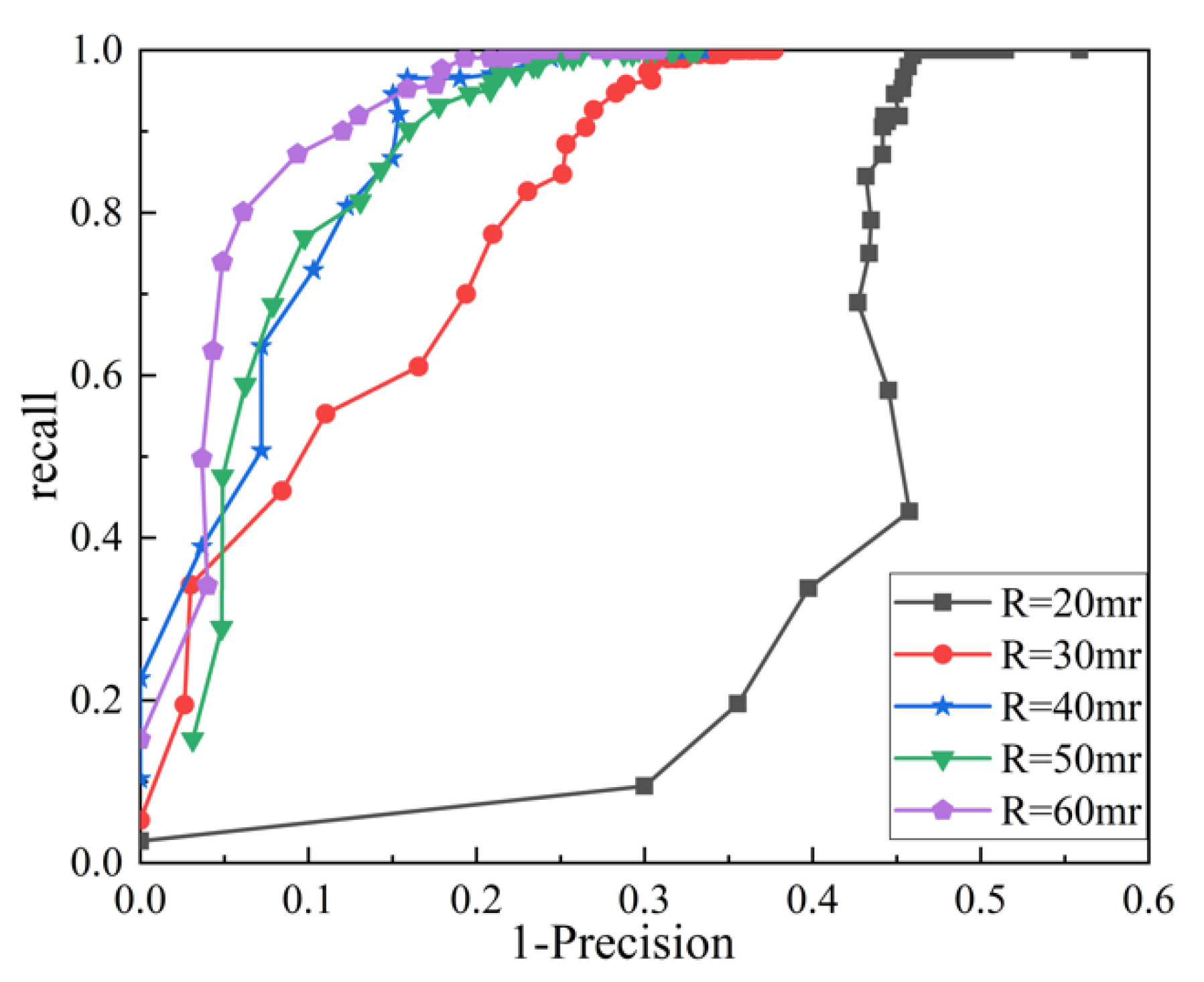
The support radius indicates the influence ability of point clouds around key points on the RSPP feature descriptors. The larger the support radius, the better the descriptors’ distinguishability, but the requirements for the repeatability of the point cloud are higher. Therefore, it is necessary to find a suitable support radius. In order to analyze the impact of different support radii on the performance of the RSPP feature descriptor, the support radius is changed, and other parameters are fixed. The specific parameter combinations are shown in

Table 1. Parameter combination of different support radii.

No	$\mathit{n}$	${\mathit{N}}_0,{\mathit{N}}_1,\dots ,{\mathit{N}}_{\mathit{n}}$	${\mathit{k}}_{\mathit{r}}^1,\dots ,{\mathit{k}}_{\mathit{r}}^{\mathit{n}}$	${\mathit{k}}_{\mathit{h}}$	$\mathit{R}$ (mr)
1	5	1, 12, 14, 16, 18, 20	1.5, 3, 5, 7, 9	1.2	20
2					30
3					40
4					50
5					60

, where mr represents the mesh resolution of the point cloud.

The RP curves of different support radii are shown in Figure 5.

It can be seen from Figure 5 that the larger the support radius, the larger the area under the RP curve, which means that the larger the support radius, the better the performance of the feature descriptor. When the support radius is 60 mr, the performance of the RSPP feature descriptor is the best.

(2) 

Radius of sampling circle

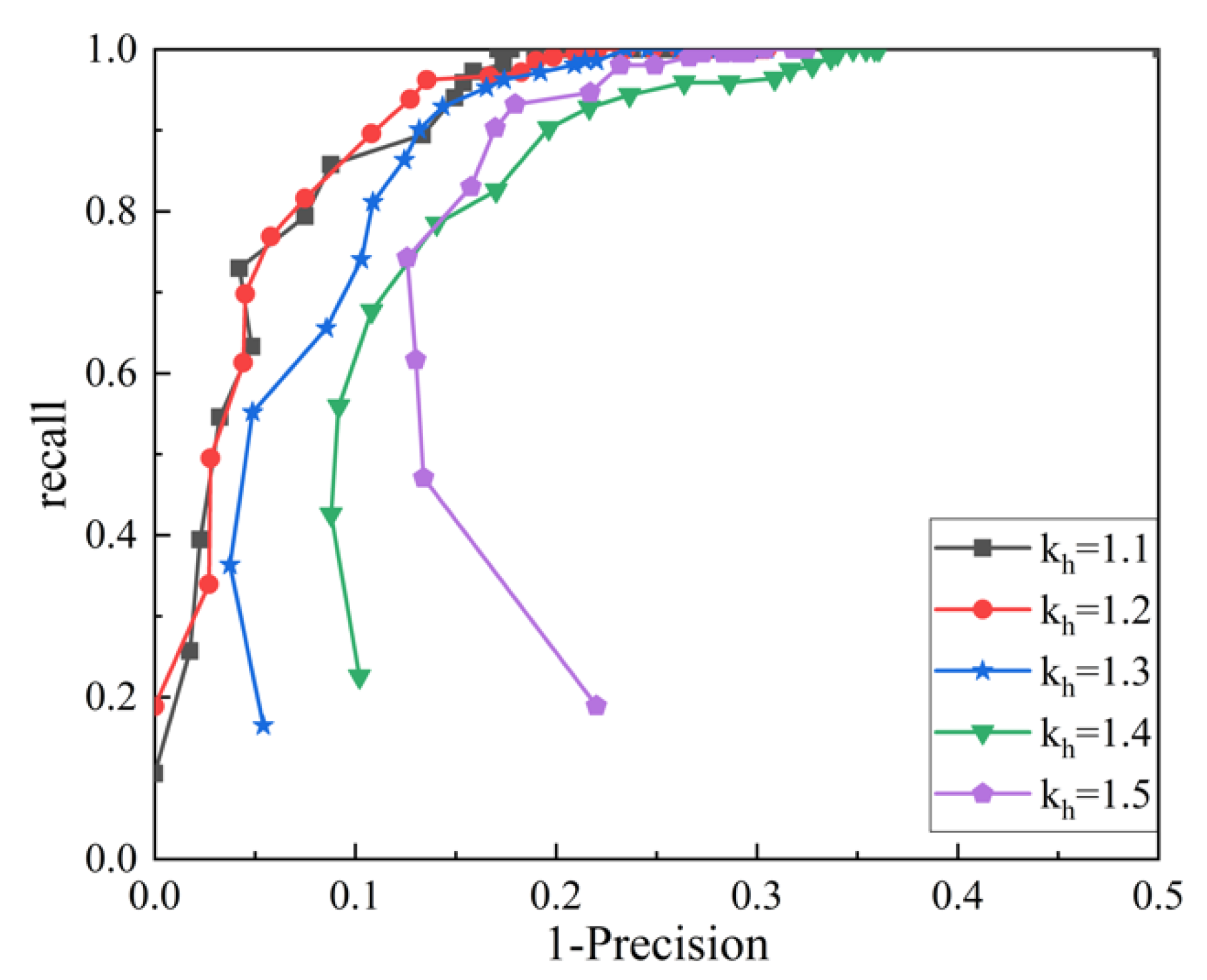
The sampling circle radius coefficient indicates the impact of different sampling layers around the key points on the RSPP feature descriptor. The larger the sampling circle radius coefficient, the smaller the impact of the point cloud in the outer layer on the descriptor. It means that the farther away from the key points, the smaller the impact on the descriptor. In order to analyze the influence of the sampling circle radius on the performance of the RSPP feature descriptor, the sampling circle radius is changed, and other parameters are fixed. The specific parameter combinations are shown in

Table 2. Parameter combination of different radii of sampling circle.

No	$\mathit{n}$	${\mathit{N}}_0,{\mathit{N}}_1,\dots ,{\mathit{N}}_{\mathit{n}}$	${\mathit{k}}_{\mathit{r}}^1,\dots ,{\mathit{k}}_{\mathit{r}}^{\mathit{n}}$	${\mathit{k}}_{\mathit{h}}$	$\mathit{R}$ (mr)
1	5	1, 12, 14, 16, 18, 20	1.5, 3, 5, 7, 9	1.1	60
2				1.2
3				1.3
4				1.4
5				1.5

.

The RP curves of different radii of sampling circle are shown in Figure 6.

It can be seen from Figure 6 that when the radius coefficient $k_h$ of the sampling circle is taken as 1.1 or 1.2, the performance of the RSPP feature descriptor is the best. In this paper, $k_h$ is taken as 1.2.

(3) 

Sampling layers

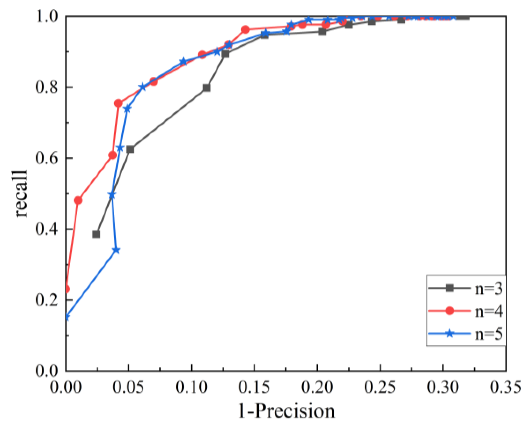
The number of sampling layers indicates the fineness of RSPP feature descriptors. The larger the number of sampling layers, the richer the point cloud details described by RSPP. In order to analyze the influence of the sampling layers on the performance of the RSPP feature descriptor, the number of sampling layers is changed, and other parameters are fixed. The specific parameter combinations are shown in

Table 3. Parameter combination of different sampling layers.

No	$\mathit{n}$	${\mathit{N}}_0,{\mathit{N}}_1,\dots ,{\mathit{N}}_{\mathit{n}}$	${\mathit{k}}_{\mathit{r}}^1,\dots ,{\mathit{k}}_{\mathit{r}}^{\mathit{n}}$	${\mathit{k}}_{\mathit{h}}$	$\mathit{R}$ (mr)
1	3	1, 12, 14, 16	1.5, 3, 5	1.2	60
2	4	1, 12, 14, 16, 18	1.5, 3, 5, 7
3	5	1, 12, 14, 16, 18, 20	1.5, 3, 5, 7, 9

.

The RP curves of different sampling layers are shown in Figure 7.

It can be seen from Figure 7 that when the number of sampling layers $n$ is 4 and 5, the performance of the RSPP feature descriptor is similar. $n$ is taken as 5 to increase the feature description ability of the descriptor in this paper.

Based on the above analysis, the combination of parameters shown in

Table 4. Parameter combination adopted in this paper.

No	$\mathit{n}$	${\mathit{N}}_0,{\mathit{N}}_1,\dots ,{\mathit{N}}_{\mathit{n}}$	${\mathit{k}}_{\mathit{r}}^1,\dots ,{\mathit{k}}_{\mathit{r}}^{\mathit{n}}$	${\mathit{k}}_{\mathit{h}}$	$\mathit{R}$ (mr)
1	5	1, 12, 14, 16, 18, 20	1.5, 3, 5, 7, 9	1.2	60

can better exert the performance of the RSPP feature descriptor.

4.4. Performance Analysis

To intuitively verify the performance of the proposed RSPP feature descriptor, the RSPP is compared with the commonly used point cloud feature descriptors, including 3DSC, SHOT, FPFH, TOLDI, and RCS. The performance of these feature descriptors under noiseless and noisy conditions is analyzed, respectively. In addition, to keep the test conditions consistent, the support radius of all feature descriptors is taken as 60 mr, as shown in

Table 5. Feature descriptor parameter Settings.

Descriptor	Support Radius (mr)	Dimension	Length	Type	Memory (Byte)
3DSC	60	15 × 12 × 11	1980	float	7920
SHOT	60	8 × 2 × 2 × 11	352	float	1408
FPFH	60	3 × 11	33	float	132
TOLDI	60	3 × 20 × 20	1200	float	4800
RCS	60	6 × 12	72	float	288
RSPP	60	3 × 81	243	binary	31

.

It can be seen from Table 5 that the binary RSPP descriptor occupies the slightest memory, which is very helpful for mobile platform applications.

(1) 

Performance analysis without noise

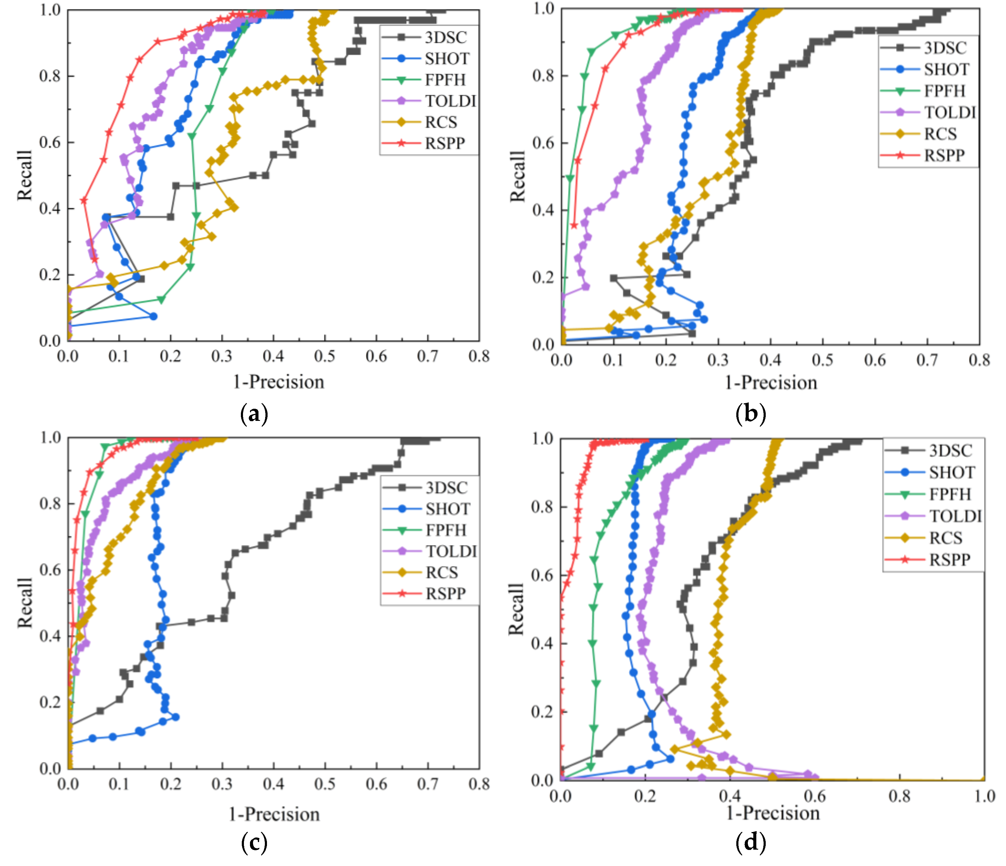
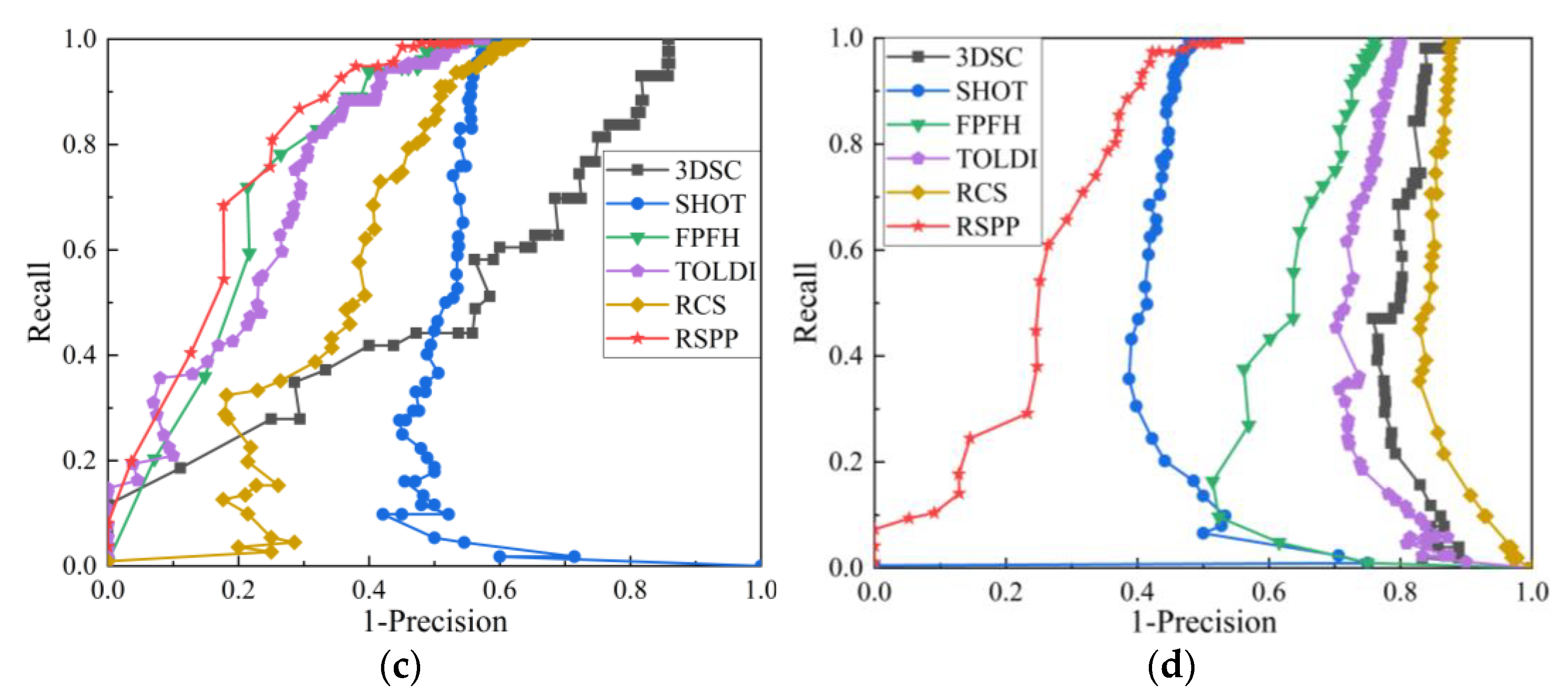
Point cloud feature extraction and matching are performed on the point cloud data of the Stanford Models without adding noise. The RP curve is shown in Figure 8.

As can be seen from Figure 8, under noise-free conditions, the RP curve of the RSPP for the Bunny and Armadillo datasets is superior to other feature descriptors, and the RP curve of the RSPP for the Buddha and Dragon datasets is close to the RP curve of FPFH and is better than other feature descriptors.

(2) 

Performance analysis with noise

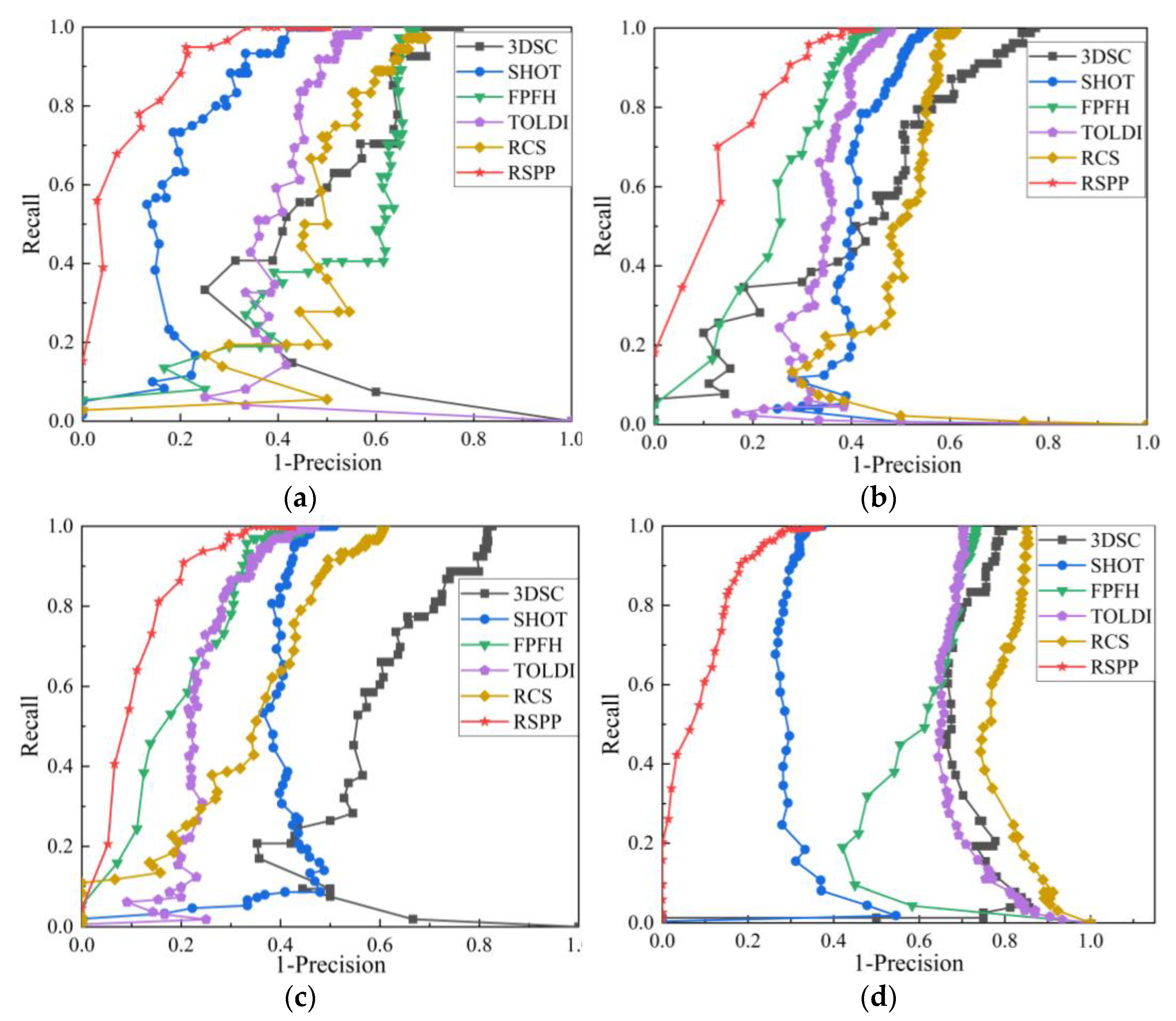
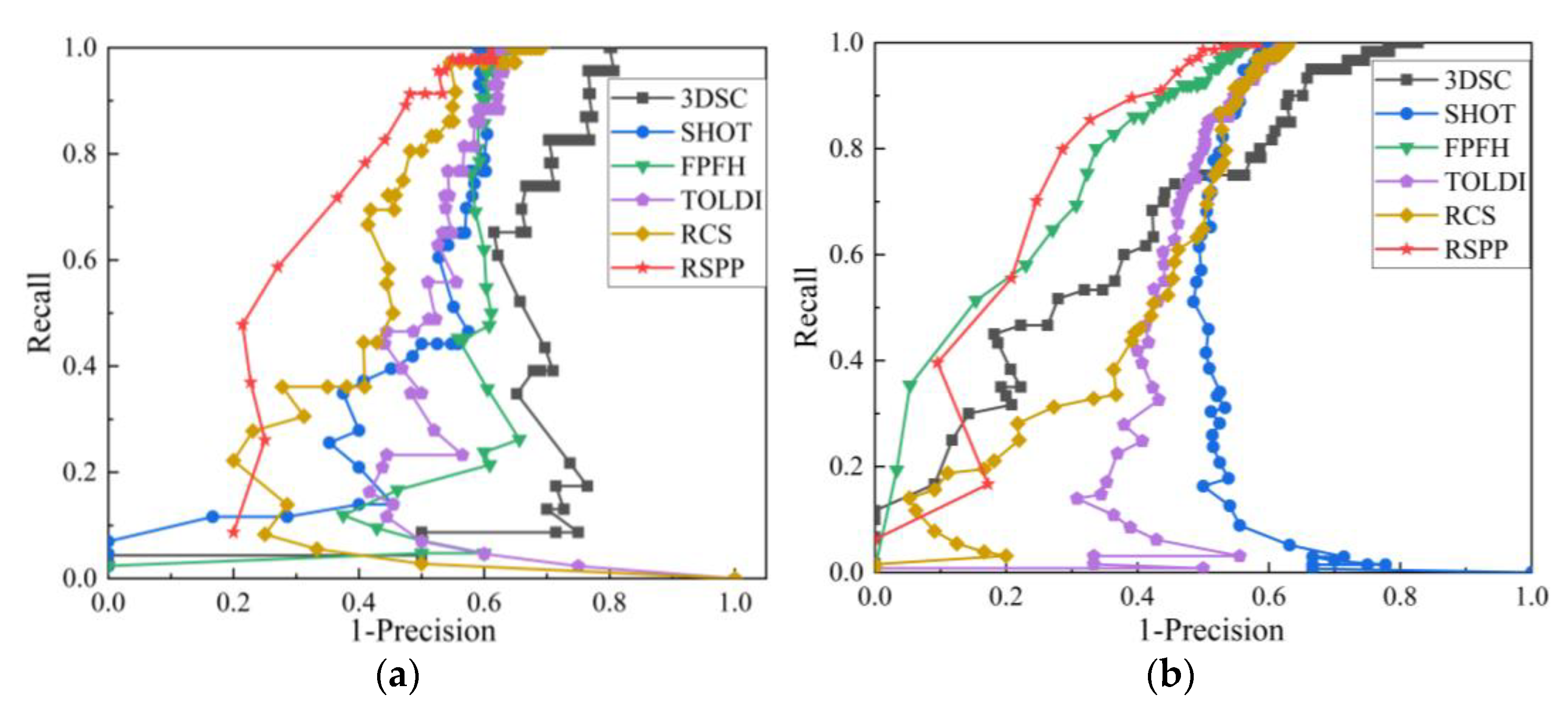
To compare the sensitivity of different point cloud feature descriptors to noise, the performance of different feature descriptors is tested when the Gaussian noise standard deviations are 0.25 mr and 0.5 mr, and their RP curves are shown in Figure 9 and Figure 10, respectively.

It can be seen from Figure 9 and Figure 10 that under the conditions of 0.25 mr and 0.5 mr Gaussian noise, the RP curves of RSPP on the test dataset are better than other feature descriptors, indicating that RSPP has good robustness against noise.

To quantitatively evaluate the accuracy of the registration algorithm, the registration accuracy of different feature descriptors under the conditions of Figure 8 to Figure 10 is calculated, as shown in

Table 6. Registration accuracy of different feature descriptors.

Gaussian Noise (mr)	Dataset	Registration Accuracy (%)
		3DSC	SHOT	FPFH	TOLDI	RCS	RSPP
0	Bunny	24.4	51.3	58.8	62.2	47.9	52.9
	Buddha	25.0	61.2	68.4	65.8	57.5	65.5
	Dragon	26.1	71.2	73.5	71.2	69.3	72.9
	Armadillo	28.3	71.7	68.9	59.2	47.9	76.5
0.25	Bunny	20.2	49.6	25.2	39.5	31.1	51.3
	Buddha	21.3	42.8	50.3	48.3	39.1	51.4
	Dragon	17.0	46.1	51.6	50.7	40.2	53.3
	Armadillo	16.8	57.6	23.7	27.9	15.0	55.5
0.5	Bunny	17.7	36.1	28.6	36.1	25.2	37.8
	Buddha	16.1	34.2	40.5	35.3	36.8	40.8
	Dragon	12.1	36.0	40.5	39.2	29.7	42.8
	Armadillo	11.3	40.6	21.7	16.4	11.3	41.2

. The two top accuracy values under different datasets in the table are displayed in bold. The distance threshold ${\epsilon }_{rmse}$ for judging whether a pair of registration points are correctly matched is 3 mr.

It can be seen from Table 6 that the proposed RSPP feature descriptor has good registration accuracy on different datasets and under different noise conditions, which verifies the accuracy and reliability of the RSPP-based point cloud registration algorithm proposed in this paper.

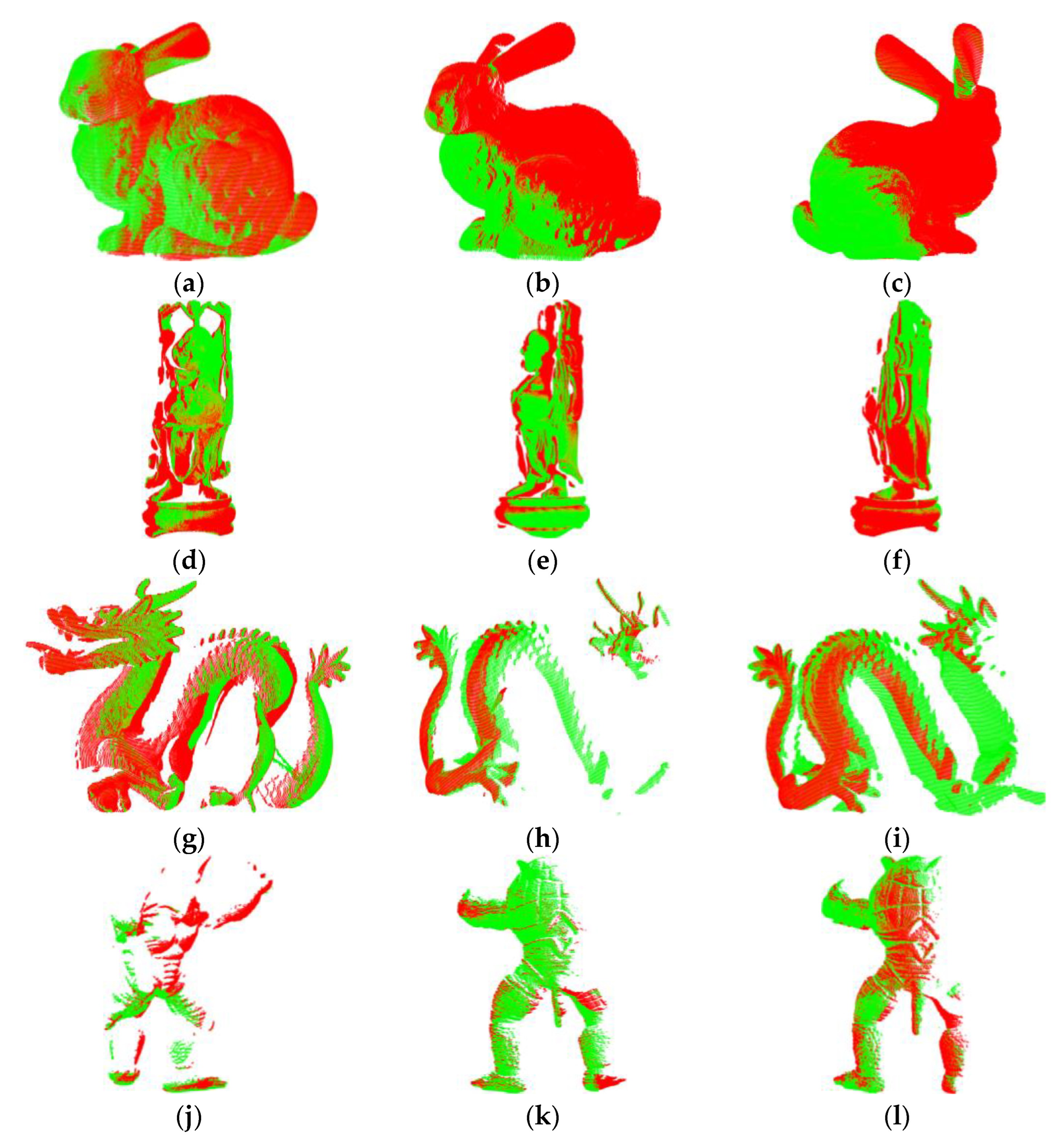
To intuitively show the effect of point cloud registration, Figure 11 shows the point cloud registration examples of different datasets. The red point represents the original point cloud, and the green point represents the registered point cloud.

It can be seen from Figure 11 that after the point cloud registration algorithm based on RSPP, the original point cloud and the registered point cloud basically coincide. Furthermore, even in the case of partial data missing and a low point cloud coincidence rate, a good registration effect can still be achieved, which intuitively verifies the performance of the registration algorithm based on the RSPP proposed in this paper.

5. Conclusions

This paper proposes a binary feature description called RSPP and an RSPP-based 3D point cloud registration algorithm to reduce the sensitivity to point cloud noise. The primary process of feature description and registration algorithm is as follows. Firstly, the key points of the input point cloud are detected, and the corresponding LRF is established. Secondly, the point cloud within the support radius around the key point is projected to the XY, YZ, and XZ planes of the LRF, and a retina-like sampling mode is established on each projection plane. At the same time, the Gaussian density weight value at the sampling point is calculated and binarized. Then, the binary Gaussian density weight value at all sampling points is encoded to obtain the RSPP feature descriptor. Finally, coarse registration of the point cloud is performed based on the RSPP descriptor, and the RANSAC algorithm is used to optimize the registration result. The performance of the proposed algorithm is tested and verified on the public Stanford 3D Scanning Repository point cloud dataset. The results show that compared with some typical point cloud feature descriptors, the RSPP-based point cloud registration algorithm has a relatively good registration effect on the test 3D point cloud datasets under noise-free, 0.25 mr, and 0.5 mr Gaussian noise conditions. It indicates that the proposed RSPP-based point cloud registration algorithm has lower sensitivity to noise, and its overall performance is better than other comparative methods. At the same time, even in the case of partial data missing and a low point cloud coincidence rate, a good registration effect can still be achieved. Furthermore, a binary RSPP feature descriptor occupies 31 bytes of memory, which is significantly smaller than other mentioned classical descriptors and has good mobile hardware application potential. The results verify the correctness and robustness of the proposed point cloud registration method, which can provide theoretical and technical support for 3D point cloud registration applications.

References

- Chiang, C.-H.; Kuo, C.-H.; Lin, C.-C.; Chiang, H.-T. 3D point cloud classification for autonomous driving via dense-residual fusion network. IEEE Access 2020, 8, 163775–163783. [Google Scholar]
- Li, X.; Du, S.; Li, G.; Li, H. Integrate point-cloud segmentation with 3D LiDAR scan-matching for mobile robot localization and mapping. Sensors 2019, 20, 237. [Google Scholar] [CrossRef] [PubMed] [Green Version]
- Qiang, L.; Ling, L. Engineering Surveying and Mapping System Based on 3D Point Cloud and Registration Communication Algorithm. Wirel. Commun. Mob. Comput. 2022, 2022, 4579565. [Google Scholar] [CrossRef]
- Zhou, K.; Ming, D.; Lv, X.; Fang, J.; Wang, M. CNN-based land cover classification combining stratified segmentation and fusion of point cloud and very high-spatial resolution remote sensing image data. Remote Sens. 2019, 11, 2065. [Google Scholar] [CrossRef] [Green Version]
- Garrido, D.; Rodrigues, R.; Augusto Sousa, A.; Jacob, J.; Castro Silva, D. Point Cloud Interaction and Manipulation in Virtual Reality. In Proceedings of the 2021 5th International Conference on Artificial Intelligence and Virtual Reality (AIVR), Kumamoto, Japan, 23–25 July 2021; pp. 15–20. [Google Scholar]
- Besl, P.J.; McKay, N.D. Method for registration of 3-D shapes. In Proceedings of the Sensor fusion IV: Control Paradigms and Data Structures, Boston, MA, USA, 2–15 November 1992; pp. 586–606. [Google Scholar]
- Yang, J.; Cao, Z.; Zhang, Q. A fast and robust local descriptor for 3D point cloud registration. Inf. Sci. 2016, 346, 163–179. [Google Scholar] [CrossRef]
- Rusu, R.B.; Blodow, N.; Marton, Z.C.; Beetz, M. Aligning point cloud views using persistent feature histograms. In Proceedings of the 2008 IEEE/RSJ International Conference on Intelligent Robots and Systems, Nice, France, 22–26 September 2008; pp. 3384–3391. [Google Scholar]
- Malassiotis, S.; Strintzis, M.G. Snapshots: A novel local surface descriptor and matching algorithm for robust 3D surface alignment. IEEE Trans. Pattern Anal. Mach. Intell. 2007, 29, 1285–1290. [Google Scholar] [CrossRef] [PubMed]
- Alahi, A.; Ortiz, R.; Vandergheynst, P. Freak: Fast retina keypoint. In Proceedings of the 2012 IEEE Conference on Computer Vision and Pattern Recognition, Providence, RI, USA, 16–21 June 2012; pp. 510–517. [Google Scholar]
- Quan, S.; Ma, J.; Hu, F.; Fang, B.; Ma, T. Local voxelized structure for 3D binary feature representation and robust registration of point clouds from low-cost sensors. Inf. Sci. 2018, 444, 153–171. [Google Scholar] [CrossRef]
- Johnson, A.E.; Hebert, M. Using spin images for efficient object recognition in cluttered 3D scenes. IEEE Trans. Pattern Anal. Mach. Intell. 1999, 21, 433–449. [Google Scholar] [CrossRef] [Green Version]
- Frome, A.; Huber, D.; Kolluri, R.; Bülow, T.; Malik, J. Recognizing objects in range data using regional point descriptors. In Proceedings of the European Conference on Computer Vision, Prague, Czech Republic, 11–14 May 2004; pp. 224–237. [Google Scholar]
- Rusu, R.B.; Blodow, N.; Beetz, M. Fast point feature histograms (FPFH) for 3D registration. In Proceedings of the 2009 IEEE International Conference on Robotics and Automation, Kobe, Japan, 12–17 May 2009; pp. 3212–3217. [Google Scholar]
- Tombari, F.; Salti, S.; Stefano, L.D. Unique signatures of histograms for local surface description. In Proceedings of the European Conference on Computer Vision, Heraklion, Greece, 5–11 September 2010; pp. 356–369. [Google Scholar]
- Guo, Y.; Sohel, F.; Bennamoun, M.; Lu, M.; Wan, J. Rotational projection statistics for 3D local surface description and object recognition. Int. J. Comput. Vis. 2013, 105, 63–86. [Google Scholar] [CrossRef] [Green Version]
- Guo, Y.; Bennamoun, M.; Sohel, F.; Lu, M.; Wan, J. 3D object recognition in cluttered scenes with local surface features: A survey. IEEE Trans. Pattern Anal. Mach. Intell. 2014, 36, 2270–2287. [Google Scholar] [CrossRef]
- Prakhya, S.M.; Lin, J.; Chandrasekhar, V.; Lin, W.; Liu, B. 3DHoPD: A fast low-dimensional 3-D descriptor. IEEE Robot. Autom. Lett. 2017, 2, 1472–1479. [Google Scholar] [CrossRef]
- Yang, J.; Zhang, Q.; Xiao, Y.; Cao, Z. TOLDI: An effective and robust approach for 3D local shape description. Pattern Recognit. 2017, 65, 175–187. [Google Scholar] [CrossRef]
- Dong, Z.; Yang, B.; Liu, Y.; Liang, F.; Li, B.; Zang, Y. A novel binary shape context for 3D local surface description. ISPRS J. Photogramm. Remote Sens. 2017, 130, 431–452. [Google Scholar] [CrossRef]
- Sun, T.; Liu, G.; Liu, S.; Meng, F.; Zeng, L.; Li, R. An efficient and compact 3D local descriptor based on the weighted height image. Inf. Sci. 2020, 520, 209–231. [Google Scholar] [CrossRef]
- Yang, J.; Zhang, Q.; Xian, K.; Xiao, Y.; Cao, Z. Rotational contour signatures for robust local surface description. In Proceedings of the 2016 IEEE International Conference on Image Processing (ICIP), Phoenix, AZ, USA, 25–28 September 2016; pp. 3598–3602. [Google Scholar]
- Quan, S.; Ma, J.; Feng, F.; Yu, K. Multi-scale binary geometric feature description and matching for accurate registration of point clouds. In Proceedings of the Fourth International Workshop on Pattern Recognition, Nanjing, China, 28–30 June 2019; pp. 112–116. [Google Scholar]
- Zhou, R.; Li, X.; Jiang, W. 3D surface matching by a voxel-based buffer-weighted binary descriptor. IEEE Access 2019, 7, 86635–86650. [Google Scholar] [CrossRef]
- Zhao, B.; Xi, J. Efficient and accurate 3D modeling based on a novel local feature descriptor. Inf. Sci. 2020, 512, 295–314. [Google Scholar] [CrossRef]
- Zou, X.; He, H.; Wu, Y.; Chen, Y.; Xu, M. Automatic 3D point cloud registration algorithm based on triangle similarity ratio consistency. IET Image Process. 2020, 14, 3314–3323. [Google Scholar] [CrossRef]
- Zhang, Y.; Li, C.; Guo, B.; Guo, C.; Zhang, S. KDD: A kernel density based descriptor for 3D point clouds. Pattern Recognit. 2021, 111, 107691. [Google Scholar] [CrossRef]
- Wang, J.; Wu, B.; Kang, J. Registration of 3D point clouds using a local descriptor based on grid point normal. Appl. Opt. 2021, 60, 8818–8828. [Google Scholar] [CrossRef]
- Sipiran, I.; Bustos, B. Harris 3D: A robust extension of the Harris operator for interest point detection on 3D meshes. Vis. Comput. 2011, 27, 963–976. [Google Scholar] [CrossRef]
- Knopp, J.; Prasad, M.; Willems, G.; Timofte, R.; Gool, L.V. Hough transform and 3D SURF for robust three dimensional classification. In Proceedings of the European Conference on Computer Vision, Heraklion, Greece, 5–11 September 2010; pp. 589–602. [Google Scholar]
- Steder, B.; Rusu, R.B.; Konolige, K.; Burgard, W. NARF: 3D range image features for object recognition. In Proceedings of the Workshop on Defining and Solving Realistic Perception Problems in Personal Robotics at the IEEE/RSJ International Conference on Intelligent Robots and Systems (IROS), Taibei, China, 18–22 October 2010. [Google Scholar]
- Zhong, Y. Intrinsic shape signatures: A shape descriptor for 3d object recognition. In Proceedings of the 2009 IEEE 12th International Conference on Computer Vision Workshops, ICCV Workshops, Kyoto, Japan, 27 September–4 October 2009; pp. 689–696. [Google Scholar]
- Leutenegger, S.; Chli, M.; Siegwart, R.Y. BRISK: Binary robust invariant scalable keypoints. In Proceedings of the 2011 International Conference on Computer Vision, Washington, DC, USA, 6–13 November 2011; pp. 2548–2555. [Google Scholar]
- Tola, E.; Lepetit, V.; Fua, P. Daisy: An efficient dense descriptor applied to wide-baseline stereo. IEEE Trans. Pattern Anal. Mach. Intell. 2009, 32, 815–830. [Google Scholar] [CrossRef] [PubMed]
- Turk, G.; Levoy, M. Zippered polygon meshes from range images. In Proceedings of the 21st Annual Conference on Computer Graphics and Interactive Techniques, Orlando, FL, USA, 24–29 July 1994; pp. 311–318. [Google Scholar]
- Curless, B.; Levoy, M. A volumetric method for building complex models from range images. In Proceedings of the 23rd Annual Conference on Computer Graphics and Interactive Techniques, Orleans, LA, USA, 4–9 August 1996; pp. 303–312. [Google Scholar]
- Krishnamurthy, V.; Levoy, M. Fitting smooth surfaces to dense polygon meshes. In Proceedings of the 23rd Annual Conference on Computer Graphics and Interactive Techniques, Vancouver, BC, Canada, 7–11 August 1996; pp. 313–324. [Google Scholar]
- Gardner, A.; Tchou, C.; Hawkins, T.; Debevec, P. Linear light source reflectometry. ACM Trans. Graph. (TOG) 2003, 22, 749–758. [Google Scholar] [CrossRef]
Figure 1.
The flow chart of the binary feature description of retina-like sampling in projection planes.
Figure 2.
Schematic diagram of the point cloud feature extraction method based on retina-like sampling on projection planes. (a) Local point cloud; (b) Sampling mode of retina-like sampling on each projection plane; (c) Sub binary feature histograms; (d) Fused binary feature histogram.