Improving Urgency-Based Backlog Sequencing of Jobs: An Assessment by Simulation

Abstract

When order release is applied, jobs are withheld in a backlog from where they are released to meet certain performance targets. The decision that selects jobs for release is typically preceded by a sequencing decision. It was traditionally assumed that backlog sequencing is only responsible for releasing jobs on time, whereas more recent literature has argued that it can also support load balancing. Although the new load-based rules outperform time-based rules, they can be criticized for requiring workload information from the shop floor and for delaying large jobs. While some jobs will inevitably be delayed during periods of high load, we argue that this delaying decision should be under control of management. A simulation study of a wafer fab environment shows that a time-based rule matches the performance of more complex load-based backlog sequencing rules that have recently emerged. The new rule realizes the lowest percentage of tardy jobs if the lower bound that distinguishes between early and urgent jobs is set appropriately. It provides a simpler means of improving release performance, allowing managers to delay jobs that have adjustable due dates.

1. Introduction

Protecting throughput from variance is the key to achieving lean [1]. If order release is applied, jobs (or orders) are not immediately released onto the shop floor upon arrival at the production system, but release is controlled to meet certain performance targets, which creates a so-called backlog or pre-shop pool that effectively buffers the shop floor. Well-known approaches to order release include Constant Work-in-Process (ConWIP; e.g., [1,2,3,4]), Drum-Buffer-Rope (DBR, e.g., [5,6,7]), and Workload Control (e.g., [8,9,10,11]), among others. Meanwhile, a similar logic is also implemented in more recent manufacturing paradigms, such as cloud manufacturing (e.g., [12,13,14,15,16,17]).

The decision concerning which jobs to release is typically subdivided into a backlog sequencing decision, which determines the sequence in which jobs are considered for release, and a selection decision, which decides for each job, in sequence, whether it should be released given certain release criteria, e.g., applying a limit to the workload released to a station. Most studies on order release have focused on the selection decision, implicitly assuming that the sequencing decision should use some measure of urgency. Only recently it has been shown that incorporating load considerations in the sequencing decision can improve performance in the context of Workload Control (e.g., [18]), ConWIP (e.g., [19]) and DBR (e.g., [20]). However, including load considerations requires feedback from the shop floor and significantly increases the complexity of the backlog sequencing decision. The challenge is whether simple time-based rules can be developed that mimic the behavior of load-based rules but without requiring regular information being fed-back from the shop floor.

Taking a closer look at load-based backlog sequencing rules reveals that they gain an advantage by delaying large jobs during periods of high load. In other words, during periods when the incoming workload largely exceeds the available capacity, load-based rules focus on producing as many small jobs on time as possible to the detriment of some large jobs. It has long since been shown that this improves overall performance [21]. In this study, we mimic this behavior by proposing a new urgency-based rule that creates three classes of jobs: early (non-urgent), urgent, and very urgent. Using a simulation model of a re-entrant flow shop [22] we conjecture that prioritizing urgent over very urgent jobs leads to similar results to those obtained for load-based sequencing, but in a simpler way.

Re-entrant flow shops are of high practical relevance. They can be found, for example, in semiconductor wafer fab environments (see e.g., [23]) and in flexible manufacturing systems (see e.g., [24]). Moreover, the advent of lean management and industry 4.0 fostered a product-based view instead of a resource-based view [25]. This enables companies to streamline their production systems, so products can be manufactured using a fixed sequence of flexible resources [26]. However, re-entrant flow shops are also very challenging environments for order release methods [27] since jobs repeatedly pass through the same station (or stations) at different stages of processing. Our new rule not only provides a simpler means of improving order release performance in such contexts, but by using dedicated classes of jobs based on urgency it also facilitates the selection of those jobs that should be delayed in practice. The new rule mainly differs from load-based rules by not requiring feedback information from the shop floor.

The remainder of this paper is structured as follows. The literature is next reviewed in Section 2 to identify the order release method and the alternative backlog sequencing rules to be considered in our study. Section 3 then outlines the simulation model used to evaluate performance before the results are presented and discussed in Section 4. Finally, Section 5 puts forward a conclusion and outlines the managerial implications and limitations of the study.

2. Literature Review

This section identifies the order release method, and the backlog sequencing rules to be included in our study in Section 2.1 and Section 2.2, respectively. A discussion of the literature is then presented in Section 2.3.

2.1. Order Release

Given its importance, several Workload Control release methods have been proposed in the literature, see e.g., the reviews by [28,29,30,31]. In this paper, we use a continuous version of Workload Control order release given its good performance in previous studies (see e.g., [32]). Workload Control restricts the load released to stations on the shop floor by load norms or load limits. Whenever a new job (or order) arrives to the production system, or whenever an operation is complete on the shop floor, the following steps are executed to decide on the release of jobs:

(1)

Jobs waiting for release in the backlog are sorted according to a sequencing rule, and the job with the highest priority is considered for release first.

(2)

If the load that results from releasing the job does not exceed the load norms for all stations in its routing, then the job is selected for release and released. Otherwise, the job remains in the backlog and the job with the next highest priority is considered for release.

(3)

The release procedure stops when all jobs in the backlog have been considered for release or when there are no more jobs in the backlog to be released.

The load contribution to a station is calculated by dividing the processing time of the operation at a station by the station’s position in a job’s routing [33]. That is, $W_s:=W_s+\frac{p_{ij}}{i}$ $\forall i\in R_j$, where $W_s$ is the workload released to station s, i is the station position in the routing of the job, $p_{ij}$ is the processing time of job j at the ith operation in its routing, and $R_j$ the set of jobs awaiting release in the backlog.

2.2. Backlog Sequencing Rules

Many backlog sequencing rules have been applied in the literature. Most of this literature has assumed that backlog sequencing is only responsible for ensuring that orders are released on time. Consequently, most studies have applied a time-oriented backlog sequencing rule. For example, refs. [18,29] used the First-Come-First-Served (FCFS) rule, a time-oriented rule that sequences jobs according to their time of arrival to the backlog. Another time-oriented rule that is widely applied, since it reflects the existence of different due date allowances across jobs, is the Earliest Due Date (EDD) rule. This rule was used by, e.g., [18,34], among others. Finally, the Planned Release Date (PRD) rule is a time-oriented rule that also reflects differences in the number of operations and the operations throughput times in the routing of jobs. It sequences jobs according to planned release dates given by Equation (1) below. Two variants of this rule are used in the literature, where either waiting times or operation throughput times are treated as a constant. This rule was used, e.g., by [11,18,29].

$${\tau }_j={\delta }_j-{{\displaystyle \sum }}_{i\in R_j}\left(a_i+p_{ij}\right) \mathrm{or} {\tau }_j={\delta }_j-{{\displaystyle \sum }}_{i\in R_j}{b}_i$$

(1)

• ${\tau }_j$ = planned release date of job j
• ${\delta }_j$ = due date of job j
• $a_i$ = estimated waiting time at the ith operation in the routing of a job
• $b_i$ = estimated throughput time at the ith operation in the routing of a job

More recently, Thürer et al. [18] questioned the assumption that backlog sequencing is mainly responsible for ensuring orders are released on time. The authors introduced a MODified Capacity Slack (MODCS) rule that combines load-balancing and urgency considerations. MODCS considers two classes of jobs, urgent and non-urgent, depending on whether jobs have a planned release date (refer to Equation (1)) that has already been passed or not. Urgent jobs have priority over non-urgent jobs. Urgent jobs are sequenced according to the Capacity Slack CORrected (CSCOR) rule. Non-urgent jobs are sequenced according to the PRD rule. CSCOR is a load-oriented rule that sequences jobs according to a capacity slack ratio, as given by Equation (2).

$$S_j^{}=\frac{{{\displaystyle \sum }}_{i\in R_j}\left(\frac{\frac{p_{ij}}{i}}{N_s^{}-W_s^{}}\right)}{n_j}$$

(2)

The capacity slack ratio integrates three elements into one priority measure: the workload contribution of a job to a station, $\frac{p_{js}}{i}$; the load gap, $N_s^{}$-$W_s^{}$ at the station that processes the ith operation of a job, and the number of operations in the routing of the job, i.e., the routing length n_j. The latter is used to average the ratio between workload contribution to stations and load gap at stations across the routing of the job. The lower the capacity slack ratio, $S_j$, the higher the priority of job j. This capacity slack rule was originally proposed by [35] and later used, e.g., by [29].

2.3. Discussion

Studies comparing the performance of different sequencing rules (e.g., [18,29]) showed that load-based rules (i.e., CS and MODCS) outperform time-based rules. However, there are two major issues. First, the CSCOR rule is rather complex and requires detailed information from the shop floor. Second, the CSCOR rule gains advantage by delaying larger jobs. This behavior is maintained also within MODCS during periods of high load when many jobs tend to become urgent. In this study we seek to address both issues by asking:

Can a new backlog sequencing rule be designed that matches the high performing MODCS rule whilst only considering job information and enabling a more controlled decision to be taken on which jobs to delay?

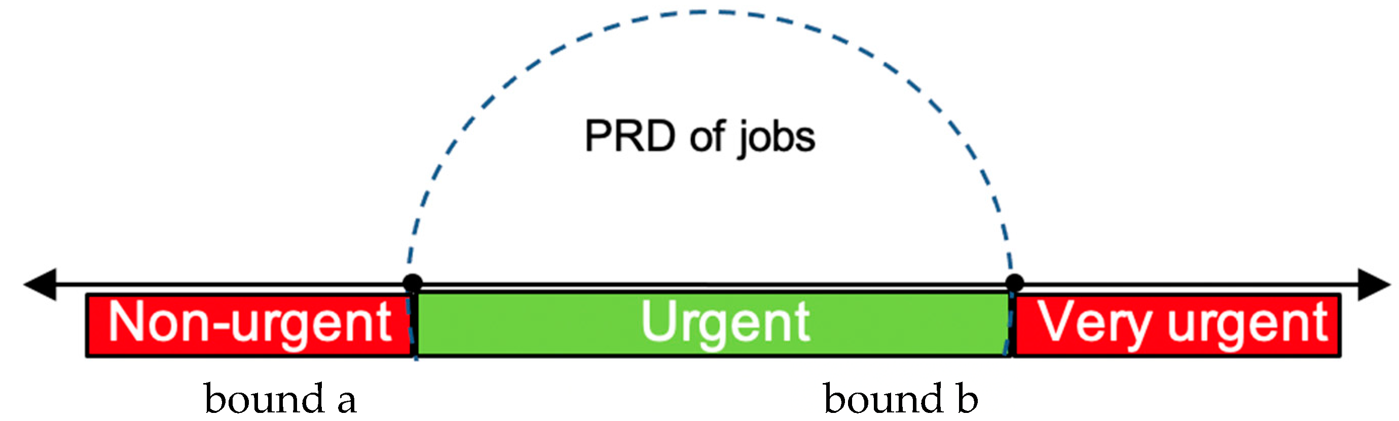
In response, we propose a new time-oriented rule. This rule creates three classes of jobs based on urgency given by the PRD of the job, as illustrated in Figure 1: early (non-urgent), urgent, and very urgent. We then conjecture that prioritizing urgent over very urgent jobs provides similar results to those obtained for MODCS, despite the relative simplicity of the new rule. The new rule differs from load-based rules as it does not require feedback information from the shop floor. It only requires a PRD to be determined for each job to create three classes of urgency that then are used to prioritize jobs. By using dedicated classes, the new rule also facilitates the selection of jobs that should be delayed in practice. In general, it should be noted that, as per the definition, some jobs will almost inevitably be delivered slowly during periods of high load [36]. The simulation model used to test our conjecture and the experimental design is outlined next in Section 3.

3. Methods

3.1. Simulation

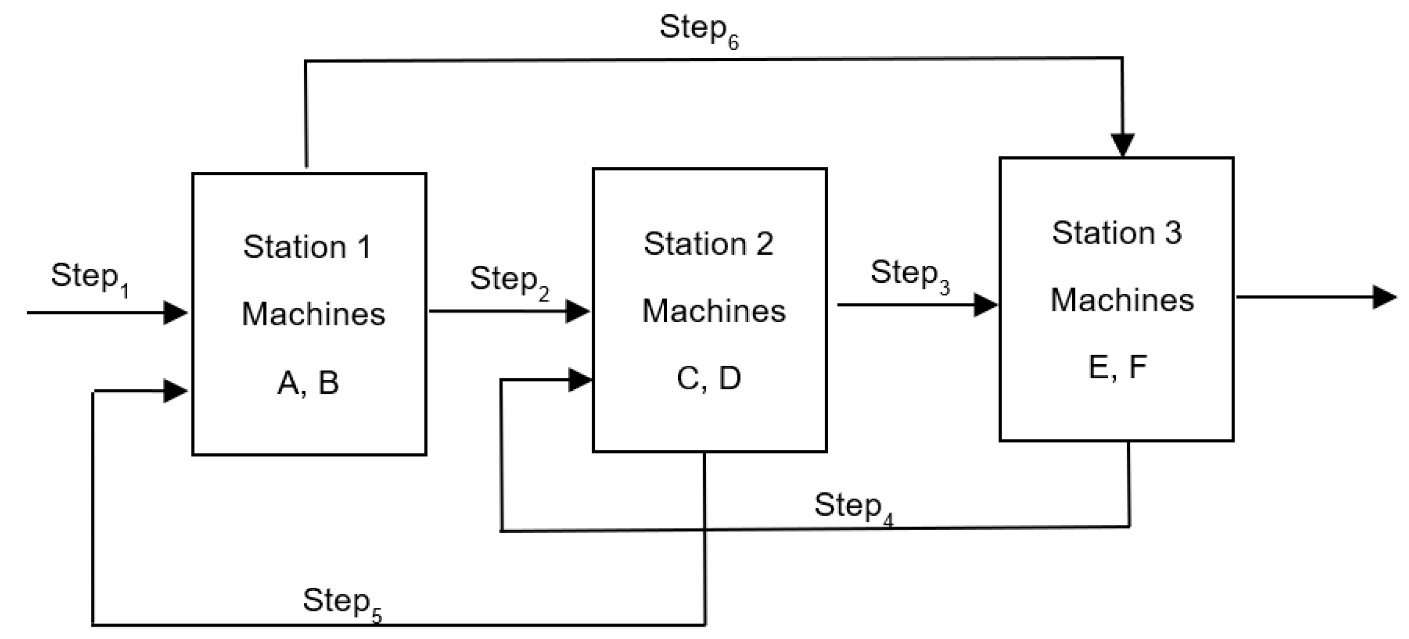
A simulation model of a re-entrant flow shop was implemented using ARENA^® software. In the model job inter-arrival times, processing times and due dates are stochastic variables. The re-entrant flow shop considered here is balanced and consists of three stations, each with two machines preceded by a single input buffer. Job routings are based on the six-step Mini-Fab model of Kempf [37], as depicted in Figure 2. That is, the production of each job is completed following a sequence of six processing steps.

In this study it is assumed that all materials for job processing are available and all the required information regarding job routings, job processing times, etc., is known at order arrival. This is in line with previous simulation studies on order release control (e.g., [10,29,38,39]). Processing times at machines follow a lognormal distribution with a mean of one time unit. Processing time variability of jobs is considered an experimental factor. We consider three levels for the coefficient of variation (CV) of the processing times, namely: 0.1, 0.2, and 0.4. We further assume that set-up times are sequence independent and considered to be part of the operation processing times. To avoid moving away from the focus of the research question and to avoid confounding factors, batch processing and unreliable machines were not considered. The inter-arrival time of jobs to the shop follows an exponential distribution. The mean of this distribution was defined to result in a system steady-state utilization rate of 90%.

Due dates are assumed to be set exogenously, i.e., by the customer. A random allowance, set between 15 and 30 time units, was added to the job entry time. Values were chosen so that releasing jobs onto the shop floor immediately upon arrival yields a percentage of tardy jobs close to 10% for an intermediate level of CV of the processing time (i.e., 0.2).

Table 1. Summary of simulated shop and job characteristics.

Shop and Job Characteristics
Routing Variability	Re-entrant flows; same sequence for all jobs
No. of Stations	3
No. of Machines	6 (two per station)
Station Capacities	All equal
Station Utilization Rate	90%
No. of Operations per Job	6
Operation Processing Times	Log-normally distributed; mean = 1
Due Date Determination	Due Date = Entry Time + d; d~U [15, 30]
Inter-Arrival Times	Exp. Distribution; mean = 1.111

summarizes the simulated shop and job characteristics.

3.2. Order Release and Backlog Sequencing

Six settings of the load norms are considered, namely, 4, 5, 6, 7, 8, and 9 time units. As a baseline setting, immediate release (IMR) of jobs to the shop floor is also considered, i.e., without controlled order release. Since EDD and PRD backlog sequencing are equivalent in shops with a single routing for all jobs, only PRD is considered. We consequently consider three backlog sequencing rules from the literature: FCFS, PRD, and MODCS. Four versions of our new rule are considered, where we change the bound a (see Figure 1) that distinguishes early (non-urgent) and urgent jobs at four levels: PRD minus an allowance of 1, 2, 5, and 10 time units, respectively. These rules are referred to as NEW (−1), NEW (−2), NEW (−5), and NEW (−10), respectively. The bound b (see Figure 1) that distinguishes between urgent and very urgent jobs is set to the PRD plus an allowance of 10 time units for all four rules based on preliminary simulation experiments, i.e., very urgent jobs are those for which the PRD is more than 10 time units in the past. Finally, the allowance for the operation throughput time at each station is set based on the cumulative moving average realized during simulation experiments.

3.3. Dispatching

Jobs waiting in the input buffer of a station are prioritized according to operation due dates. The operation due date for the last operation in the routing of a job is equal to the due date of the job, as given by Equation (1), while the operation due date of each preceding operation is determined by successively subtracting the estimated station waiting time and processing time from the operation due date of the next operation. In this study, estimated station waiting times are given by the cumulative moving average, i.e., the average of all station waiting times realized until the current simulation time.

3.4. Experimental Design and Performance Measures

Our study considers three experimental factors tested at different levels: (i) three levels of processing time variability (CV = 0.1, 0.2, and 0.4); (ii) six levels of the workload norm (4, 5, 6, 7, 8, and 9 time units); and (iii) seven backlog sequencing rules. A full factorial design was used with 126 (3 × 6 × 7) experimental scenarios, where each scenario was run for 13,000 time units following a warm-up period of 3000 time units. Each experimental scenario was replicated 100 times. These simulation conditions allow for obtaining stable results with small (i.e., precise) confidence intervals for the performance measures.

The key performance measures considered are the total throughput time, the percentage of tardy jobs, and the mean tardiness. The total throughput time refers to the time that elapses between job entry to the system and job completion. The percentage of tardy jobs refers to the percentage of jobs completed after their due date. Tardiness is defined to be zero if the job is on time or early and it is equal to the completion date minus the due date if the job is late. In addition, we also measure the average shop floor throughput time, which is used as an instrumental performance variable. While the total throughput time includes the time that jobs wait before being released, i.e., the backlog waiting time, the shop floor throughput time refers to the time that elapses between job release to the shop floor and job completion.

4. Results and Discussion

An initial statistical analysis of simulation results was conducted using an ANOVA (Analysis of Variance). ANOVA results are presented in

Table 2. ANOVA results.

	Source of Variance	Sum of Squares	Degrees of Freedom	Mean Squares	F-Ratio	p-Value
Percentage Tardy	Coefficient of Variation (CV)	18,370.15	2	9185.07	1142.61	0.00
	Norm	17,638.49	5	3527.70	438.84	0.00
	Pool Sequencing (S)	34,028.43	6	5671.40	705.51	0.00
	CV × Norm	2114.88	10	211.49	26.31	0.00
	CV × S	1706.67	12	142.22	17.69	0.00
	Norm × S	7315.81	30	243.86	30.34	0.00
	CV × Norm × S	415.26	60	6.92	0.86	0.77
	Error	100,266.43	12,473	8.04
Mean Tardiness	Coefficient of Variation (CV)	418.28	2	209.14	1270.57	0.00
	Norm	408.90	5	81.78	496.84	0.00
	Pool Sequencing (S)	229.63	6	38.27	232.51	0.00
	CV × Norm	161.29	10	16.13	97.99	0.00
	CV × S	0.48	12	0.04	0.24	1.00
	Norm × S	130.72	30	4.36	26.47	0.00
	CV × Norm × S	3.90	60	0.07	0.40	1.00
	Error	2053.07	12,473	0.16
Total Throughput Time	Coefficient of Variation (CV)	5585.58	2	2792.79	3435.25	0.00
	Norm	400.46	5	80.09	98.52	0.00
	Pool Sequencing (S)	18.12	6	3.02	3.71	0.00
	CV × Norm	124.71	10	12.47	15.34	0.00
	CV × S	9.12	12	0.76	0.93	0.51
	Norm × S	3.00	30	0.10	0.12	1.00
	CV × Norm × S	1.00	60	0.02	0.02	1.00
	Error	10,140.30	12,473	0.81
Shop Floor Throughput Time	Coefficient of Variation (CV)	1865.34	2	932.67	6782.66	0.00
	Norm	18,268.67	5	3653.73	26,571.01	0.00
	Pool Sequencing (S)	3.40	6	0.57	4.12	0.00
	CV × Norm	256.49	10	25.65	186.53	0.00
	CV × S	0.80	12	0.07	0.49	0.92
	Norm × S	0.24	30	0.01	0.06	1.00
	CV × Norm × S	0.08	60	0.00	0.01	1.00
	Error	1715.14	12,473	0.14

. All main effects and most of the two-way interactions were found to be statistically significant. There were no significant three-way interactions.

As somewhat expected from the choice and the design of our backlog sequencing rules, the backlog sequencing rules have the strongest impact on the percentage tardy and mean tardiness. This can also be observed from the results for the Scheffé multiple comparison procedure, which was applied to obtain a first indication of the direction and size of the performance differences.

Table 3. Results for Scheffé multiple comparison procedure.

Rule (x)	Rule (y)	Percentage Tardy		Mean Tardiness		Total Throughput Time		Shop Floor Throughput Time
		Lower (1)	Upper	Lower	Upper	Lower	Upper	Lower	Upper
NEW (−2)	NEW (−1) (2)	−0.92	−0.25	−0.03 *	0.07	−0.12 *	0.10	−0.05 *	0.04
NEW (−5)	NEW (−1)	−2.12	−1.45	0.08	0.18	−0.14 *	0.07	−0.06 *	0.03
NEW (−10)	NEW (−1)	−2.49	−1.82	0.34	0.43	−0.15 *	0.06	−0.08 *	0.01
MODCS	NEW (−1)	0.17	0.84	−0.07 *	0.03	−0.12 *	0.09	−0.04 *	0.05
PRD	NEW (−1)	1.85	2.52	−0.06 *	0.04	−0.05 *	0.16	−0.02 *	0.06
FCFS	NEW (−1)	2.06	2.73	−0.03 *	0.06	−0.05 *	0.17	−0.05 *	0.04
NEW (−5)	NEW (−2)	−1.54	−0.87	0.06	0.16	−0.13 *	0.08	−0.06 *	0.03
NEW (−10)	NEW (−2)	−1.90	−1.23	0.32	0.41	−0.14 *	0.07	−0.08 *	0.01
MODCS	NEW (−2)	0.76	1.43	−0.09 *	0.01	−0.11 *	0.10	−0.03 *	0.05
PRD	NEW (−2)	2.43	3.11	−0.08 *	0.01	−0.04 *	0.17	−0.02 *	0.07
FCFS	NEW (−2)	2.65	3.32	−0.05 *	0.04	−0.04 *	0.18	−0.04 *	0.04
NEW (−10)	NEW (−5)	−0.70	−0.03	0.20	0.30	−0.12 *	0.10	−0.06 *	0.03
MODCS	NEW (−5)	1.96	2.63	−0.20	−0.10	−0.09 *	0.13	−0.02 *	0.07
PRD	NEW (−5)	3.63	4.31	−0.19	−0.10	−0.02 *	0.20	−0.01 *	0.08
FCFS	NEW (−5)	3.85	4.52	−0.16	−0.07	−0.01 *	0.20	−0.03 *	0.06
MODCS	NEW (−10)	2.33	3.00	−0.45	−0.36	−0.08 *	0.14	0.00	0.08
PRD	NEW (−10)	4.00	4.67	−0.44	−0.35	−0.01 *	0.21	0.01	0.10
FCFS	NEW (−10)	4.22	4.89	−0.42	−0.32	0.00	0.21	−0.01 *	0.08
PRD	MODCS	1.34	2.01	−0.04 *	0.06	−0.04 *	0.18	−0.03 *	0.06
FCFS	MODCS	1.55	2.23	−0.01 *	0.08	−0.03 *	0.18	−0.05 *	0.04
FCFS	PRD	−0.12 *	0.55	−0.02 *	0.08	−0.10 *	0.11	−0.07 *	0.02

⁽¹⁾ 95% confidence interval; ⁽²⁾ allowance for bound that distinguishes early jobs; * not significant at 0.05.

gives the 95% confidence interval. When this interval includes zero, performance differences are not considered to be statistically significant. We can observe significant performance differences for all pairs for at least one performance measure except for between FCFS and PRD, for which performance is statistically equivalent. This is explored further in Section 4.1 and Section 4.2 where detailed performance results are presented and their robustness evaluated.

4.1. Performance Assessment

Results for a coefficient of variation (CV) of the processing times of 0.1 together with the 95% confidence intervals are given in

Table 4. Simulation results for jobs CV = 0.1.

	Load Norm	STT (1)	TTT (2)	T (3)	P (4) (%)
IMR	None	13.35 ± 0.18	13.35 ± 0.18	0.39 ± 0.07	7.85 ± 0.73
FCFS	4	09.30 ± 0.02	12.62 ± 016	0.42 ± 0.07	7.20 ± 0.61
	5	10.34 ± 0.04	12.75 ± 0.16	0.34 ± 0.06	6.60 ± 0.59
	6	11.14 ± 0.06	12.99 ± 0.16	0.33 ± 0.06	6.80 ± 0.62
	7	11.67 ± 0.07	13.12 ± 0.16	0.34 ± 0.06	7.00 ± 0.63
	8	12.02 ± 0.09	13.18 ± 0.17	0.35 ± 0.06	7.17 ± 0.65
	9	12.26 ± 0.10	13.22 ± 0.17	0.36 ± 0.06	7.31 ± 0.66
PRD	4	09.30 ± 0.02	12.58 ± 016	0.34 ± 0.06	6.25 ± 0.60
	5	10.36 ± 0.04	12.77 ± 0.16	0.31 ± 0.06	6.17 ± 0.61
	6	11.17 ± 0.06	13.00 ± 0.16	0.32 ± 0.06	6.65 ± 0.63
	7	11.70 ± 0.08	13.14 ± 0.16	0.34 ± 0.06	7.02 ± 0.65
	8	12.06 ± 0.09	13.21 ± 0.17	0.35 ± 0.06	7.26 ± 0.66
	9	12.31 ± 0.10	13.25 ± 0.17	0.36 ± 0.06	7.42 ± 0.67
MODCS	4	09.30 ± 0.02	12.56 ± 0.15	0.36 ± 0.06	4.25 ± 0.39
	5	10.35 ± 0.04	12.74 ± 0.15	0.30 ± 0.06	5.22 ± 0.51
	6	11.16 ± 0.06	12.98 ± 0.16	0.31 ± 0.06	6.27 ± 0.60
	7	11.69 ± 0.07	13.11 ± 0.16	0.32 ± 0.06	6.82 ± 0.63
	8	12.05 ± 0.09	13.18 ± 0.16	0.34 ± 0.06	7.13 ± 0.65
	9	12.31 ± 0.10	13.23 ± 0.17	0.35 ± 0.06	7.35 ± 0.66
NEW (−10) (1)	4	09.29 ± 0.02	12.64 ± 0.15	1.17 ± 0.12	3.74 ± 0.16
	5	10.32 ± 0.04	12.74 ± 0.15	0.88 ± 0.09	3.06 ± 0.15
	6	11.14 ± 0.06	12.98 ± 0.16	0.72 ± 0.08	2.75 ± 0.15
	7	11.68 ± 0.07	13.11 ± 0.16	0.60 ± 0.07	2.93 ± 0.21
	8	12.03 ± 0.09	13.17 ± 0.16	0.51 ± 0.07	3.45 ± 0.29
	9	12.28 ± 0.10	13.21 ± 0.17	0.45 ± 0.07	4.32 ± 0.38
NEW (−5)	4	09.29 ± 0.02	12.58 ± 0.17	0.57 ± 0.09	2.24 ± 0.17
	5	10.34 ± 0.04	12.74 ± 0.16	0.44 ± 0.07	2.18 ± 0.18
	6	11.14 ± 0.06	12.98 ± 0.16	0.39 ± 0.07	3.07 ± 0.29
	7	11.68 ± 0.07	13.11 ± 0.16	0.36 ± 0.06	4.50 ± 0.43
	8	12.04 ± 0.09	13.18 ± 0.16	0.36 ± 0.06	5.64 ± 0.51
	9	12.30 ± 0.10	13.22 ± 0.17	0.36 ± 0.06	6.46 ± 0.59
NEW (−2)	4	09.30 ± 0.02	12.58 ± 0.17	0.43 ± 0.09	2.59 ± 0.21
	5	10.35 ± 0.04	12.74 ± 0.16	0.35 ± 0.07	3.21 ± 0.31
	6	11.15 ± 0.06	12.98 ± 0.16	0.33 ± 0.07	4.84 ± 0.47
	7	11.68 ± 0.07	13.11 ± 0.16	0.32 ± 0.06	6.03 ± 0.56
	8	12.04 ± 0.09	13.18 ± 0.16	0.34 ± 0.06	6.67 ± 0.61
	9	12.30 ± 0.10	13.22 ± 0.17	0.35 ± 0.06	7.10 ± 0.64
NEW (−1)	4	09.30 ± 0.02	12.58 ± 0.17	0.39 ± 0.07	3.24 ± 0.31
	5	10.35 ± 0.04	12.74 ± 0.16	0.32 ± 0.06	4.25 ± 0.46
	6	11.15 ± 0.06	12.98 ± 0.16	0.32 ± 0.06	5.72 ± 0.55
	7	11.69 ± 0.07	13.12 ± 0.16	0.33 ± 0.06	6.54 ± 0.60
	8	12.04 ± 0.09	13.19 ± 0.16	0.34 ± 0.06	6.96 ± 0.63
	9	12.30 ± 0.10	13.23 ± 0.17	0.35 ± 0.06	7.26 ± 0.65

⁽¹⁾ Shop Throughput Time; ⁽²⁾ Total Throughput Time. ⁽³⁾ Tardiness ⁽⁴⁾ Percentage of Tardy Jobs.

. Results for different levels of the CVs are presented as part of our robustness analysis in Section 4.2.

For IMR, the percentage of tardy jobs is about 8%. When jobs are not retained in a pool before release, the shop and the total throughput times are identical (13.35 time units). However, when controlled job release is applied and workload norms are tightened, the workload on the shop floor is restricted, and the shop throughput time is reduced. For example, shop throughput time is reduced to 9.30 time units when the load norm is restricted to 4 time units under FCFS, i.e., a reduction of about 30%. This has a positive impact not only on total throughput times, but also on the percentage of tardy jobs if the workload norm is set appropriately. However, when norms are set too tightly, there may be an increase in the percentage of tardy jobs because the time in the pool offsets the reduction in shop floor throughput times, and there is an increase in sequencing deviations. That is, when norms are set too tightly some jobs may be delayed for long periods in the pre-shop pool (or backlog) before being released to the shop floor, which increases the mean tardiness. Results also confirm previous literature in the sense that PRD outperforms FCFS at tighter norms, and MODCS outperforms PRD. Since the superior performance of PRD over FCFS only occurs at tighter norms, it was found not to be statistically significant in our ANOVA.

Most importantly, our new backlog sequencing rule has the potential to outperform existing backlog sequencing rules if the lower bound that distinguishes between early and urgent jobs is set appropriately. The results further highlight that there is no best rule for all performance measures. NEW (−5) allows the lowest percentage of tardy jobs to be obtained, while NEW (−1) approaches the tardiness values of MODCS and PRD. Meanwhile, if the lower bound is set to be too large/loose (i.e., PRD minus 10 time units), then we increase the set of urgent jobs to include some jobs that are still early. As a result, the number of very urgent jobs is likely to increase, resulting in worse performance. This can be observed from

Table 5. Distribution of the number of tardy jobs for a workload norm of 4 time units.

Lateness	FCFS	PRD	MODCS	New (−10)	New (−5)	New (−2)	New (−1)
]0,10]	497	399	298	155	120	180	212
]10,20]	50	48	23	63	29	23	33
]20,30]	1	3	10	46	24	16	16
]30,40]	0	0	6	24	23	12	14
]40,50]	0	1	3	20	8	10	5
]50,60]	0	0	3	16	2	2	2
]60,∞]	0	0	3	23	15	4	2
Total	548	451	346	347	221	247	284

, which provides more detailed information on the tardiness of jobs for a workload norm level of 4 time units.

The results in Table 5 highlight that: (i) both MODCS and our new rule improve overall performance by delaying some jobs and (ii) it is important for our new rule to capture only the jobs that are at risk of becoming tardy and still have a chance of being delivered on time as part of the urgent class of jobs that are released first.

4.2. Robustness Analysis

The relative performance of the different backlog sequencing rules is also not affected by the CV of the processing times. This can be observed from

Table 6. Simulation results for CV = 0.2.

	Load Norm	STT (1)	TTT (2)	T (3)	P (4) (%)
IMR	None	14.09 ± 0.20	14.09 ± 0.20	0.52 ± 0.08	9.96 ± 0.85
FCFS	4	09.49 ± 0.03	13.58 ± 0.21	0.74 ± 0.09	9.96 ± 0.70
	5	10.68 ± 0.04	13.52 ± 0.18	0.51 ± 0.08	8.55 ± 0.70
	6	11.56 ± 0.06	13.68 ± 0.18	0.46 ± 0.07	8.55 ± 0.71
	7	12.17 ± 0.08	13.81 ± 0.18	0.46 ± 0.07	8.80 ± 0.74
	8	12.60 ± 0.10	13.90 ± 0.18	0.47 ± 0.07	9.08 ± 0.76
	9	12.92 ± 0.11	13.95 ± 0.18	0.48 ± 0.07	9.34 ± 0.77
PRD	4	09.48 ± 0.03	13.49 ± 0.20	0.64 ± 0.09	8.85 ± 0.70
	5	10.70 ± 0.04	13.51 ± 0.18	0.46 ± 0.07	8.08 ± 0.71
	6	11.59 ± 0.06	13.69 ± 0.18	0.44 ± 0.07	8.43 ± 0.74
	7	12.20 ± 0.08	13.82 ± 0.18	0.45 ± 0.07	8.80 ± 0.75
	8	12.63 ± 0.10	13.91 ± 0.18	0.47 ± 0.07	9.16 ± 0.76
	9	12.95 ± 0.11	13.97 ± 0.19	0.48 ± 0.07	9.41 ± 0.78
MODCS	4	09.47 ± 0.03	13.40 ± 0.19	0.71 ± 0.09	5.23 ± 0.33
	5	10.69 ± 0.04	13.44 ± 0.17	0.46 ± 0.07	5.40 ± 0.44
	6	11.57 ± 0.06	13.62 ± 0.17	0.42 ± 0.06	6.70 ± 0.57
	7	12.18 ± 0.08	13.77 ± 0.17	0.42 ± 0.06	7.86 ± 0.65
	8	12.60 ± 0.09	13.86 ± 0.17	0.44 ± 0.07	8.59 ± 0.70
	9	12.94 ± 0.11	13.93 ± 0.18	0.45 ± 0.07	9.11 ± 0.75
NEW (−10) (1)	4	09.44 ± 0.02	13.42 ± 0.20	1.60 ± 0.14	4.85 ± 0.18
	5	10.64 ± 0.04	13.40 ± 0.17	1.09 ± 0.10	3.78 ± 0.17
	6	11.53 ± 0.06	13.58 ± 0.17	0.85 ± 0.09	3.29 ± 0.17
	7	12.14 ± 0.07	13.72 ± 0.17	0.66 ± 0.08	3.63 ± 0.25
	8	12.58 ± 0.09	13.83 ± 0.17	0.59 ± 0.07	4.94 ± 0.40
	9	12.90 ± 0.11	13.87 ± 0.18	0.53 ± 0.07	6.27 ± 0.53
NEW (−5)	4	09.47 ± 0.03	13.42 ± 0.19	1.07 ± 0.11	3.91 ± 0.19
	5	10.66 ± 0.04	13.41 ± 0.17	0.72 ± 0.09	2.97 ± 0.18
	6	11.55 ± 0.06	13.60 ± 0.17	0.58 ± 0.07	3.29 ± 0.25
	7	12.16 ± 0.08	13.74 ± 0.17	0.51 ± 0.07	4.81 ± 0.40
	8	12.60 ± 0.09	13.84 ± 0.17	0.48 ± 0.07	6.45 ± 0.55
	9	12.91 ± 0.11	13.90 ± 0.18	0.47 ± 0.07	7.67 ± 0.64
NEW (−2)	4	09.48 ± 0.03	13.43 ± 0.20	0.81 ± 0.10	4.00 ± 0.24
	5	10.68 ± 0.04	13.44 ± 0.17	0.53 ± 0.07	3.74 ± 0.30
	6	11.56 ± 0.06	13.63 ± 0.17	0.47 ± 0.07	5.05 ± 0.44
	7	12.17 ± 0.08	13.77 ± 0.17	0.45 ± 0.07	6.75 ± 0.58
	8	12.61 ± 0.09	13.86 ± 0.17	0.45 ± 0.07	7.94 ± 0.66
	9	12.92 ± 0.11	13.92 ± 0.18	0.45 ± 0.07	8.70 ± 0.71
NEW (−1)	4	09.47 ± 0.03	13.44 ± 0.19	0.74 ± 0.09	4.45 ± 0.28
	5	10.68 ± 0.04	13.45 ± 0.17	0.49 ± 0.07	4.56 ± 0.38
	6	11.56 ± 0.06	13.63 ± 0.17	0.44 ± 0.07	6.05 ± 0.51
	7	12.18 ± 0.08	13.78 ± 0.17	0.44 ± 0.07	7.46 ± 0.63
	8	12.62 ± 0.10	13.87 ± 0.18	0.44 ± 0.07	8.36 ± 0.69
	9	12.93 ± 0.11	13.93 ± 0.18	0.46 ± 0.07	8.95 ± 0.74

⁽¹⁾ Shop Throughput Time; ⁽²⁾ Total Throughput Time. ⁽³⁾ Tardiness ⁽⁴⁾ Percentage of Tardy Jobs.

and

Table 7. Simulation results for CV = 0.4.

	Load Norm	STT (1)	TTT (2)	T (3)	P (4) (%)
IMR	None	16.36 ± 0.26	16.36 ± 0.26	1.10 ± 0.13	17.97 ± 1.00
FCFS	4	09.20 ± 0.03	17.50 ± 0.44	2.95 ± 0.29	18.09 ± 1.05
	5	11.38 ± 0.05	15.52 ± 0.24	1.27 ± 0.12	11.73 ± 0.75
	6	12.53 ± 0.07	15.49 ± 0.20	0.95 ± 0.10	11.79 ± 0.80
	7	13.41 ± 0.09	15.66 ± 0.21	0.87 ± 0.10	13.03 ± 0.87
	8	14.08 ± 0.11	15.83 ± 0.22	0.86 ± 0.10	14.49 ± 0.95
	9	14.58 ± 0.13	15.96 ± 0.22	0.90 ± 0.10	15.50 ± 0.98
PRD	4	09.90 ± 0.03	17.38 ± 0.41	2.79 ± 0.27	17.13 ± 1.03
	5	11.39 ± 0.05	15.50 ± 0.24	1.21 ± 0.12	11.43 ± 0.77
	6	12.56 ± 0.07	15.49 ± 0.22	0.92 ± 0.10	11.78 ± 0.82
	7	13.45 ± 0.09	15.68 ± 0.22	0.87 ± 0.10	13.33 ± 0.91
	8	14.11 ± 0.11	15.85 ± 0.22	0.88 ± 0.10	14.66 ± 0.97
	9	14.61 ± 0.13	15.98 ± 0.22	0.91 ± 0.10	15.67 ± 0.99
MODCS	4	09.87 ± 0.03	16.92 ± 0.36	2.87 ± 0.29	09.82 ± 0.38
	5	11.36 ± 0.05	15.29 ± 0.22	1.26 ± 0.12	06.54 ± 0.33
	6	12.52 ± 0.07	15.32 ± 0.20	0.91 ± 0.09	07.53 ± 0.46
	7	13.40 ± 0.09	15.51 ± 0.20	0.80 ± 0.08	10.23 ± 0.65
	8	14.06 ± 0.11	15.70 ± 0.20	0.79 ± 0.09	12.64 ± 0.81
	9	14.55 ± 0.13	15.85 ± 0.21	0.82 ± 0.09	14.42 ± 0.89
NEW (−10) (1)	4	09.81 ± 0.03	16.99 ± 0.39	4.12 ± 0.33	08.22 ± 0.24
	5	11.27 ± 0.04	15.19 ± 0.22	1.89 ± 0.15	05.81 ± 0.20
	6	12.42 ± 0.06	15.19 ± 0.19	1.30 ± 0.11	04.98 ± 0.22
	7	13.31 ± 0.08	15.41 ± 0.19	1.02 ± 0.09	06.21 ± 0.35
	8	13.98 ± 0.11	15.61 ± 0.20	0.89 ± 0.09	09.36 ± 062
	9	14.48 ± 0.12	15.78 ± 0.20	0.86 ± 0.09	12.19 ± 0.79
NEW (−5)	4	09.85 ± 0.03	16.91 ± 0.37	3.41 ± 0.29	07.68 ± 0.26
	5	11.32 ± 0.04	15.21 ± 0.21	1.55 ± 0.13	05.16 ± 0.21
	6	12.47 ± 0.06	15.24 ± 0.19	1.09 ± 0.10	05.04 ± 0.26
	7	13.35 ± 0.09	15.46 ± 0.19	0.90 ± 0.09	07.45 ± 0.47
	8	14.01 ± 0.11	15.66 ± 0.20	0.84 ± 0.09	10.75 ± 070
	9	14.51 ± 0.12	15.81 ± 0.21	0.84 ± 0.09	13.11 ± 0.84
NEW (−2)	4	09.87 ± 0.03	16.98 ± 0.37	3.03 ± 0.27	08.35 ± 0.31
	5	11.34 ± 0.05	15.28 ± 0.22	1.35 ± 0.12	05.48 ± 0.25
	6	12.50 ± 0.07	15.29 ± 0.20	0.97± 0.07	05.19 ± 0.39
	7	13.38 ± 0.09	15.50 ± 0.20	0.84 ± 0.09	09.03 ± 0.59
	8	14.04 ± 0.11	15.70 ± 0.20	0.81 ± 0.09	12.00 ± 079
	9	14.54 ± 0.13	15.85 ± 0.21	0.83 ± 0.09	14.05 ± 0.88
NEW (−1)	4	09.78 ± 0.03	17.00 ± 0.37	2.93 ± 0.26	08.99 ± 0.35
	5	11.36 ± 0.05	15.31 ± 0.22	1.30 ± 0.12	05.97 ± 0.30
	6	12.51 ± 0.07	15.32 ± 0.20	0.94± 0.09	06.86 ± 0.43
	7	13.38 ± 0.09	15.51 ± 0.20	0.82 ± 0.09	09.63 ± 0.63
	8	14.05 ± 0.11	15.71 ± 0.20	0.81 ± 0.09	12.43 ± 0.80
	9	14.55 ± 0.13	15.86 ± 0.21	0.83 ± 0.09	14.30 ± 0.89

⁽¹⁾ Shop Throughput Time; ⁽²⁾ Total Throughput Time. ⁽³⁾ Tardiness ⁽⁴⁾ Percentage of Tardy Jobs.

, which give the results for a CV of 0.2 and 0.4, respectively. The main effect of the CV is on the best-performing norm level. The best-performing norm level in terms of the mean tardiness remains at five time units, but for the percentage of tardy jobs, the best-performing norm level increases with the coefficient of variation since we also observe less of an impact on the total throughput time and percentage of tardy jobs with an increase in the CV. A higher variability in processing times increases the load balancing opportunities for the release method, which in turn provides ‘less room’ for the sequencing rules.

5. Conclusions

Load-based backlog sequencing rules were recently highlighted as an important means to improve order release performance. However, they rely on feedback information from the shop floor and they delay jobs with long processing times during periods of high loads. In answer to our research question—Can a new backlog sequencing rule be designed that matches high performing MODCS rule whilst only considering job information and enabling a more controlled decision to be taken on which job to delay?—we have shown that similar performance can be achieved in our simulations by simply subdividing orders in the backlog into early, urgent, and very urgent orders, and then releasing urgent before very urgent orders.

Our new, purely time-oriented rule not only provides a simpler means of improving order release performance, using dedicated classes, but it also facilitates the selection of jobs that are desirable to delay. This allows managers in practice to delay specific jobs for which customer due dates can be adjusted. It puts the control of which jobs to delay in the hand of managers. In fact, it may be an alternative explanation for the Workload Control paradox, which recognizes that order release methods often perform better in practice than expected given their simulation results [40]. Managers in practice are likely to show exactly this behavior–agreeing on new due date allowances for jobs that are otherwise ‘hopelessly’ delayed.

A main limitation of our study is that we have only focused on one order release method. Although this is justified by Workload Control arguably being the best order release method for high-variety contexts, future research could assess the impact of our new rule on the performance of alternative release methods, such as ConWIP and DBR. Another limitation is that the study only considered the specific case of a re-entrant flow shop. Future research could consider other shop configurations, e.g., flow shops and job shops. Meanwhile, a main advantage of our new method is that it uses dedicated job classes to determine which jobs should be delayed. This allows for delaying jobs with flexible customer due dates as part of the due date negotiation process.

References

- Hopp, W.J.; Spearman, M.L. To pull or not to pull: What is the question? Manuf. Serv. Oper. Manag. 2004, 6, 133–148. [Google Scholar] [CrossRef] [Green Version]
- Spearman, M.L.; Woodruff, D.L.; Hopp, W.J. CONWIP: A pull alternative to Kanban. Int. J. Prod. Res. 1990, 28, 879–894. [Google Scholar] [CrossRef]
- Prakash, J.; Chin, J.F. Modified CONWIP systems: A review and classification. Prod. Plan. Control 2015, 26, 296–307. [Google Scholar] [CrossRef]
- Jaegler, Y.; Jaegler, A.; Burlat, P.; Lamouri, S.; Trentesaux, D. The CONWIP production control system: A systematic review and classification. Int. J. Prod. Res. 2018, 56, 5736–5757. [Google Scholar] [CrossRef]
- Goldratt, E.M.; Cox, J. The Goal: Excellence in Manufacturing; North River Press: Great Barrington, MA, USA, 1984. [Google Scholar]
- Simons, J.V.; Simpson, W.P., III. An exposition of multiple constraint scheduling as implemented in the goal system (formerly disaster). Prod. Oper. Manag. 1997, 6, 3–22. [Google Scholar] [CrossRef]
- Watson, K.J.; Blackstone, J.H.; Gardiner, S.C. The evolution of a management philosophy: The theory of constraints. J. Oper. Manag. 2007, 25, 387–402. [Google Scholar] [CrossRef]
- Cigolini, R.; Portioli-Staudacher, A. An experimental investigation on workload limiting methods with ORR policies in a job shop environment. Prod. Plan. Control 2002, 13, 602–613. [Google Scholar] [CrossRef]
- Portioli-Staudacher, A.; Tantardini, M. A lean-based ORR system for non-repetitive manufacturing. Int. J. Prod. Res. 2011, 50, 3257–3273. [Google Scholar] [CrossRef] [Green Version]
- Thürer, M.; Stevenson, M.; Silva, C.; Land, M.J.; Fredendall, L.D. Workload control (WLC) and order release: A lean solution for make-to-order companies. Prod. Oper. Manag. 2012, 21, 939–953. [Google Scholar] [CrossRef]
- Haeussler, S.; Netzer, P. Comparison between rule-and optimization-based workload control concepts: A simulation optimization approach. Int. J. Prod. Res. 2020, 58, 3724–3743. [Google Scholar] [CrossRef]
- Delaram, J.; Houshamand, M.; Ashtiani, F.; Fatahi Valilai, O. Development of public cloud manufacturing markets: A mechanism design approach. Int. J. Syst. Sci. Oper. Logist. 2022, 1–27. [Google Scholar] [CrossRef]
- Delaram, J.; Houshamand, M.; Ashtiani, F.; Valilai, O.F. A utility-based matching mechanism for stable and optimal resource allocation in cloud manufacturing platforms using deferred acceptance algorithm. J. Manuf. Syst. 2021, 60, 569–584. [Google Scholar] [CrossRef]
- Wu, S.; Cao, H.; Zhao, H.; Hu, Y.; Yang, L.; Yin, H.; Zhu, H. A softwarized resource allocation framework for security and location guaranteed services in B5G networks. Comput. Commun. 2021, 178, 26–36. [Google Scholar] [CrossRef]
- Liu, Y.; Xu, X.; Zhang, L.; Wang, L.; Zhong, R.Y. Workload-based multi-task scheduling in cloud manufacturing. Robot. Comput. Integr. Manuf. 2017, 45, 3–20. [Google Scholar] [CrossRef]
- Soualhia, M.; Khomh, F.; Tahar, S. Task scheduling in big data platforms: A systematic literature review. J. Syst. Softw. 2017, 134, 170–189. [Google Scholar] [CrossRef] [Green Version]
- Xu, X.; Cao, L.; Wang, X. Adaptive task scheduling strategy based on dynamic workload adjustment for heterogeneous Hadoop clusters. IEEE Syst. J. 2014, 10, 471–482. [Google Scholar] [CrossRef]
- Thürer, M.; Land, M.J.; Stevenson, M.; Fredendall, L.D.; Godinho Filho, M. Concerning Workload Control and Order Release: The Pre-Shop Pool Sequencing Decision. Prod. Oper. Manag. 2015, 24, 1179–1192. [Google Scholar] [CrossRef]
- Thürer, M.; Fernandes, N.O.; Stevenson, M.; Qu, T. On the Backlog-sequencing Decision for Extending the Applicability of ConWIP to High-Variety Contexts: An Assessment by Simulation. Int. J. Prod. Res. 2017, 55, 4695–4711. [Google Scholar] [CrossRef] [Green Version]
- Thürer, M.; Stevenson, M. On the Beat of the Drum: Improving the Flow Shop Performance of the Drum-Buffer-Rope Scheduling Mechanism. Int. J. Prod. Res. 2018, 56, 3294–3305. [Google Scholar] [CrossRef] [Green Version]
- Land, M.J.; Su, N.P.B.; Gaalman, G.J.C. In search of the key to delivery improvement. In Proceedings of the 16th International Working Seminar on Production Economics, Innsbruck, Austria, 1–5 March 2010; Volume 2, pp. 297–308. [Google Scholar]
- Graves, S.C.; Meal, H.C.; Stefek, D.; Zeghmi, A.H. Scheduling of Re-Entrant Flow Shops. J. Oper. Manag. 1983, 3, 197–207. [Google Scholar] [CrossRef]
- Muhammad, N.A.; Chin, J.F.; Kamarrudin, S.; Chik, M.A.; Prakash, J. Fundamental simulation studies of CONWIP in front-end wafer fabrication. J. Ind. Prod. Eng. 2015, 32, 232–246. [Google Scholar] [CrossRef]
- Rifai, A.P.; Dawal, S.Z.M.; Zuhdi, A.; Aoyama, H.; Case, K. Reentrant FMS scheduling in loop layout with consideration of multi loading-unloading stations and shortcuts. Int. J. Adv. Manuf. Technol. 2016, 82, 1527–1545. [Google Scholar] [CrossRef]
- Fullerton, R.R.; Kennedy, F.A.; Widener, S.K. Lean manufacturing and firm performance: The incremental contribution of lean management accounting practices. J. Oper. Manag. 2014, 32, 414–428. [Google Scholar] [CrossRef]
- Kundu, K.; Land, M.J.; Portioli-Staudacher, A.; Bokhorst, J.A.C. Order review and release in make-to-order flow shops: Analysis and design of new methods. Flex. Serv. Manuf. J. 2021, 33, 750–782. [Google Scholar] [CrossRef]
- Neuner, P.; Haeussler, S. Rule based workload control in semiconductor manufacturing revisited. Int. J. Prod. Res. 2021, 59, 5972–5991. [Google Scholar] [CrossRef]
- Wisner, J.D. A review of the order release policy research. Int. J. Oper. Prod. Manag. 1995, 15, 25–40. [Google Scholar] [CrossRef]
- Fredendall, L.D.; Ojha, D.; Patterson, J.W. Concerning the theory of workload control. Eur. J. Oper. Res. 2010, 201, 99–111. [Google Scholar] [CrossRef]
- Bagni, G.; Godinho Filho, M.; Thürer, M.; Stevenson, M. Systematic Review and Discussion of Production Control Systems that emerged between 1999 and 2018. Prod. Plan. Control, 2021; in print. [Google Scholar] [CrossRef]
- Gómez Paredes, F.; Godinho Filho, M.; Thürer, M.; Fernandes, N.O.; Jabbour, C.J.C. Factors for choosing Production Control Systems in Make-To-Order Shops: A Systematic Literature Review. J. Intell. Manuf. 2022, 33, 639–674. [Google Scholar] [CrossRef]
- Fernandes, N.O.; Carmo-Silva, S. Workload Control under continuous order release. Int. J. Prod. Econ. 2011, 131, 257–262. [Google Scholar] [CrossRef]
- Oosterman, B.; Land, M.J.; Gaalman, G. The influence of shop characteristics on workload control. Int. J. Prod. Econ. 2000, 68, 107–119. [Google Scholar] [CrossRef] [Green Version]
- Philipoom, P.R.; Steele, D.C. Shop floor control when tacit worker knowledge is important. Decis. Sci. 2011, 42, 655–688. [Google Scholar] [CrossRef]
- Philipoom, P.R.; Malhotra, M.K.; Jensen, J.B. An evaluation of capacity sensitive order review and release procedures in job shops. Decis. Sci. 1993, 24, 1109–1133. [Google Scholar] [CrossRef]
- Land, M.J.; Stevenson, M.; Thürer, M.; Gaalman, G.J.C. Job Shop Control: In Search of the Key to Delivery Improvements. Int. J. Prod. Econ. 2015, 168, 257–266. [Google Scholar] [CrossRef] [Green Version]
- Kempf, K. Intel Five-Machine Six Step Mini-Fab Description. 1994. Available online: https://aar.faculty.asu.edu/research/intel/papers/fabspec.html (accessed on 30 April 2020).
- Thürer, M.; Fernandes, N.O.; Ziengs, N.; Stevenson, M. On the meaning of ConWIP cards: An assessment by simulation. J. Ind. Prod. Eng. 2019, 36, 49–58. [Google Scholar] [CrossRef] [Green Version]
- Fernandes, N.O.; Martins, T.; Carmo-Silva, S. Improving materials flow through autonomous production control. J. Ind. Prod. Eng. 2018, 35, 319–327. [Google Scholar] [CrossRef]
- Bertrand, J.W.M.; van Ooijen, H.P.G. Workload Control order release and productivity: A missing link. Prod. Plan. Control 2002, 13, 665–678. [Google Scholar] [CrossRef]
Figure 1.
Classes of jobs based on urgency.
Figure 2.
Illustration of the re-entrant flow shop under study.