
A p−V Diagram Based Fault Identification for Compressor Valve by Means of Linear Discrimination Analysis


1
School of Energy and Power Engineering, Xi’an Jiaotong University, Xi’an 710049, China
2
Operation District of Hutubi Gas Storage, PetroChina Xinjiang Oilfield Company, Hutubi 831200, China
3
State Key Laboratory of Multiphase Flow in Power Engineering, Xi’an Jiaotong University, Xi’an 710049, China
*
Author to whom correspondence should be addressed.
Machines 2022, 10(1), 53; https://doi.org/10.3390/machines10010053
Submission received: 8 December 2021
/
Revised: 29 December 2021
/
Accepted: 5 January 2022
/
Published: 10 January 2022
(This article belongs to the Special Issue Fault Diagnosis and Health Management of Power Machinery)
Abstract
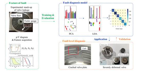
:The pressure-volume diagram (p−V diagram) is an established method for analyzing the thermodynamic process in the cylinder of a reciprocating compressor as well as the fault of its core components including valves. The failure of suction/discharge valves is the most common cause of unscheduled shutdowns, and undetected failure may lead to catastrophic accidents. Although researchers have investigated fault classification by various estimation techniques and case studies, few have looked deeper into the barriers and pathways to realize the level determination of faults. The initial stage of valve failure is characterized in the form of mild leakage; if this is identified at this period, more serious accidents can be prevented. This study proposes a fault diagnosis and severity estimation method of the reciprocating compressor valve by virtue of features extracted from the p−V diagram. Four-dimensional characteristic variables consisting of the pressure ratio, process angle coefficient, area coefficient, and process index coefficient are extracted from the p−V diagram. Principal Component Analysis (PCA) and Linear Discriminant Analysis (LDA) were applied to establish the diagnostic model, where PCA realizes feature amplification and projection, then LDA implements feature dimensionality reduction and failure prediction. The method was validated by the diagnosis of various levels of severity of valve leakage in a reciprocating compressor, and further, applied in the diagnosis of two actual faults: Mild leakage caused by the cracked valve plate in a reciprocating compressor, and serious leakage caused by the deformed valve in a hydraulically driven piston compressor for a hydrogen refueling station (HRS).
1. Introduction
The reciprocating compressor is one of the most used kernel equipment in the energy transmission field to acquire high-pressure gas [1]. Despite the popularity, some vulnerable components including self-acting valves, piston rods, and crossheads usually result in the unplanned downtime of the compressor, which brings considerable negative effects to the industrial application. The failure can lead to a chain reaction that causes the system to run abnormally and hereby result in heavy casualties and negative social impacts. According to the statistics provided by PROGNOST [2], an investigation on the most common failure mode of reciprocating compressors showed that valve failure is the main reason for the unplanned shutdown of the compressor. Some surveys indicated that valve failures accounted for 60% of the unit failures, whose maintenance costs accounted for 36% of the total operation and maintenance expenditure [3,4].
Valves are of great significance for reciprocating compressors, for they control the working process of the compressor, and they are also the main source of the compressor power loss [5]. The cleanliness of gas flow is an important factor influencing valve failure, and liquid and debris can considerably shorten the service life of the valve. Although early valve leakage is usually not related to safety, undetected valve failure may lead to complete compression failure, which can lead to severe damage and accidents. For example, for a double-acting compressor, the dynamic piston rod load changes periodically between tension and compression, yielding a gap between the crosshead bearing bush and the pin to provide space for lubrication. The insufficient reverse force and/or angles will lead to poor lubrication at the crosshead as well as redundant heat, resulting in more catastrophic failures such as the stick and wear of the crosshead pin and bearing bush. Hence, real-time monitoring and fault diagnosis is necessary for the application of the reciprocating compressor.
Although new valve structures and improved materials are gradually introduced, and the failure rate is greatly reduced, for many compressor operators, condition monitoring of valves is still the main approach to reduce unplanned downtime [6]. Hitherto, various physical state parameters have been used to diagnose the status of the compressor. Zhou et al. [7] provided an adaptive Generative Adversarial Network to enhance the weak fault features of the vibration signal to complete fault diagnosis of a natural gas compressor. Liang et al. [8] took the advantage of modal analysis, calculation of the resonant piping length, velocity frequency spectrum analysis, and pressure pulsation measurement to solve the abnormal vibration of reciprocating compressor inlet pipelines. Townsend et al. [9] designed temperature-monitoring devices on the connecting rods and validated the availability. Becerra et al. [10] analyzed the premature failure of crankshafts based on the inner cylinder pressure. Ghamry [11] and Wang [12] et al. proposed and used acoustic emission (AE) technology to realize the condition monitoring and fault diagnosis of the compressor. Chlumsky [13] indicated pressure can diagnose faults of the leakage valve, piston ring, and delayed closing of discharge valves based on experimental research. Manepatil et al. [14] proved the viability of pressure pulsation on piston rod failure. Elhaj et al. [15] combined the pressure and instantaneous angular velocity (IAS) to form two truth tables for diagnosis. Most of the previous studies on compressor valve failure have focused on the classification of valve failure types, such as valve cracks, valve deformation, and foreign matter jams. However, the initial stage of valve failure is characterized in the form of leakage; if the failure is identified at this initial stage, to a large extent, more serious accidents can be avoided.
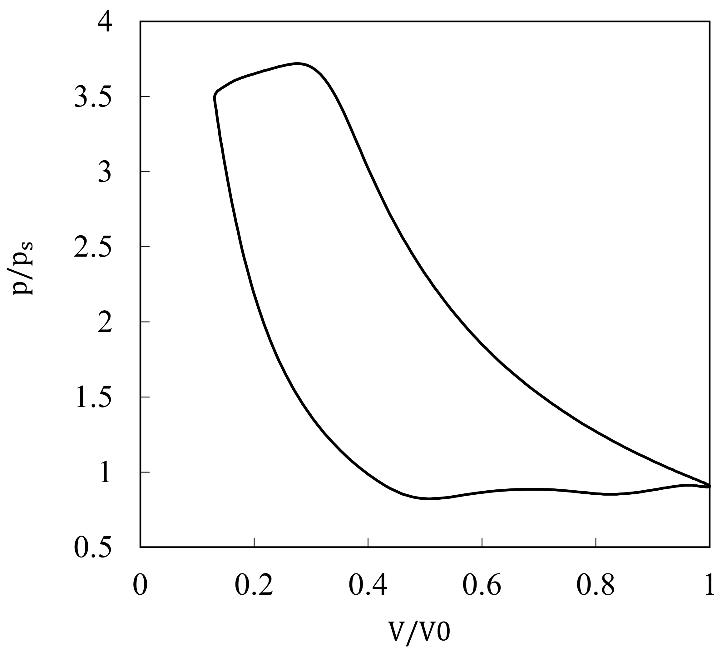
The pressure-volume (p−V) diagram can reflect the performance and status of the reciprocating compressor comprehensively, whose abscissa is the cylinder volume and ordinate is the inside pressure. The p−V diagram can indicate the problems during the working process of the compressor in an all-around way. Real et al. [16] showed the behavior and performance of discharge can be evaluated by the p−V diagram and valve displacement signal. The shape of the p−V diagram is used to diagnose operating information such as leakage faults, pressure fluctuations, and heat exchange conditions. Kim et al. [17] employed the pressure inside the cylinder to perform valve dynamic analysis considering heat transform to obtain the efficiency of the compressor. Li et al. [18] proposed a strain-based method to record the p−V diagram of the reciprocating compressor by measuring the piston rod strain and validated the method by the diagnosis of valve leakage. In industrial applications, the p−V diagram is the must-have function in the online monitoring systems developed by Windrock [19], HOERBIGER [20], PROGNOST [21], and Bently Nevada [22]. However, the application of the p−V diagram requires qualified expertise and experience. Therefore, there is a strong need to simplify the approach to enable relatively low-skilled operators to use p−V diagrams flexibly.
Data-driven methods play an increasingly efficient role in the establishment of fault diagnosis models, which can determine the potential connections between massive amounts of data and machines. Principal Component Analysis (PCA), Linear Discriminant Analysis (LDA), Support Vector Machine (SVM), and so on have been used for fault classification by processing vibration and pressure signals in the reciprocating compressor and other kinds of industrial applications. Ahmed et al. [23] applied PCA to select features of a time-domain vibration signal to realize fault identification of suction valve leakage, inter-cooler leakage, loose drive belt, and multi-fault conditions. Wang et al. [24] induced LDA to determine the influence of each variable to assign a corresponding weight for the maximum mean discrepancy for deep transfer network, which showed better generalization ability and classification accuracy. Wang et al. [25] integrated the p−V diagram and SVM by means of image-processing methods to obtain seven invariant moments of the p−V diagram, which diagnose five kinds of faults of the valve. Feng et al. [26] chose the discrete 2D-Curvelet transform to mine the features of the p−V diagram, and the PCA was adapted to conduct novelty detection. The fault classification was realized by SVM. Pichler et al. [27] paid attention to the expansion period of the p−V diagram and used the linearized logp−V diagram to extract the gradient as a feature. The SVM was conducted to classify the fault types of valves. There is no denying that most of the solutions do realize the identification of types and components of faults, but few are involved in the estimation of fault severity, according to which manufacturers could develop maintenance plans and inventory allocation of spare components more conveniently.
In this paper, a fault diagnosis and severity estimation method of the reciprocating compressor valve by virtue of features extracted from the p−V diagram is proposed. First, the p−V diagrams of different levels of leakage fault were obtained by the experimental mock-up. Second, four-dimensional characteristic variables, composed of the pressure ratio, process angle coefficient, p−V area coefficient, and process index coefficient, were extracted from the p−V diagram to characterize the valve operating state. Next, through a combination of PCA and LDA, the diagnostic model was established, where PCA is used to project and amplify the features of characteristic variables preliminarily. The LDA is used for the first time for dimensionality reduction of p−V diagram feature variables, in order to predict the level of a valve leakage fault. Further, the feasibility and accuracy of this method were validated by the identification of different levels of valve leakage faults in a reciprocating compressor. Eventually, this method was also applied in the fault diagnosis of the failure induced by the cracked valve plate in the reciprocating compressor and the deformed valve plate in the hydraulically driven piston compressor.
2. Methodology
2.1. Acquisition of p−V Diagram
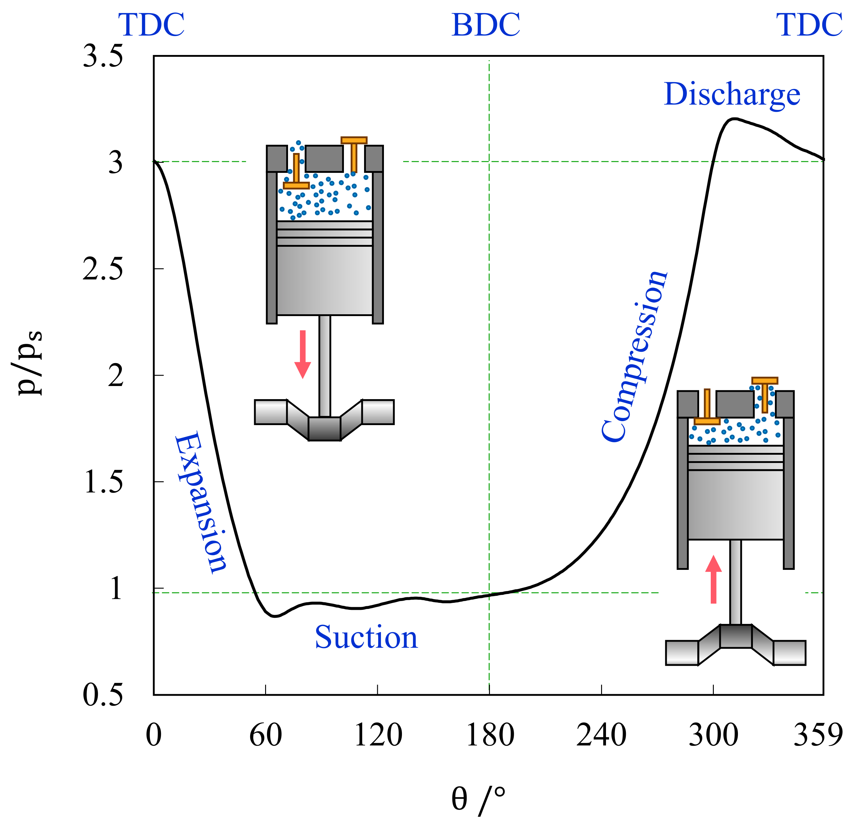
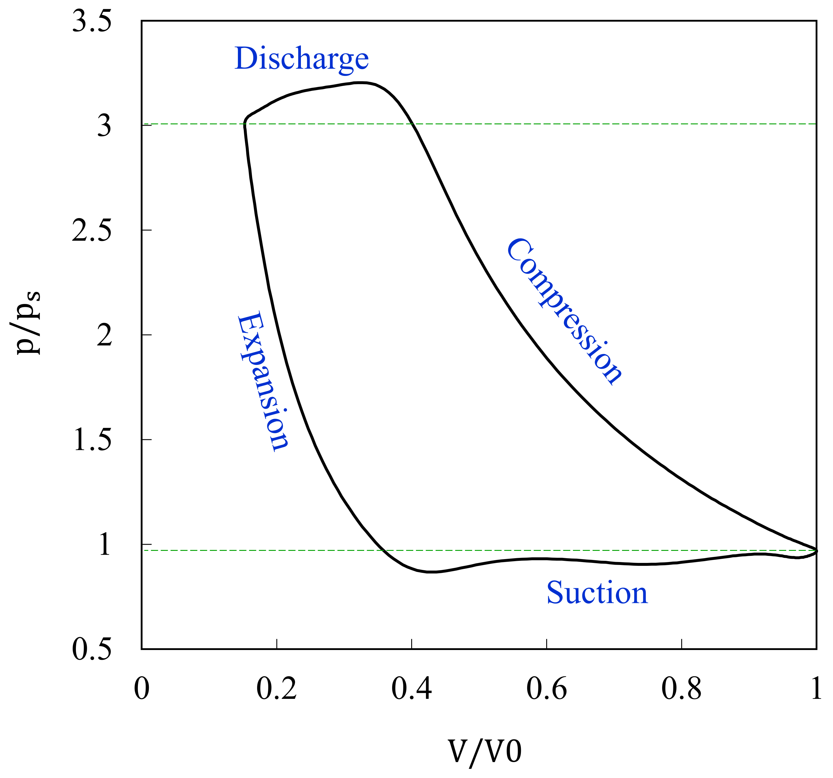
A reciprocating compressor is a positive displacement machine wherein a volume of gas is drawn into a compressor cylinder’s compression chamber where it is trapped, compressed, and pushed out. Based on the measured top dead center (TDC) of the piston movement, the angle-domain signal (i.e., time-domain) of the pressure in the cylinder (i.e., the p−θ diagram in Figure 1) can be converted into a pressure-volume diagram (i.e., the p−V diagram in Figure 2).
Figure 3 shows the schematic diagram of a reciprocating compressor. The position of the piston is determined by the crank angle. The top dead center (TDC) is set as the origin of coordinates of the piston displacement.
The working volume of the cylinder can be calculated from
where is the clearance volume, is the cylinder diameter, is the length of the connecting rod, is the crank radius, is the ratio of the crank radius to the length of the connecting rod, and is the crank angle.
Taking the working volume as the abscissa and the pressure as the ordinate, the p−V diagram can be obtained [28].
2.2. Feature Extraction of p−V Diagram
2.2.1. Selection of Statistical Characteristic Parameters of the p−V Diagram
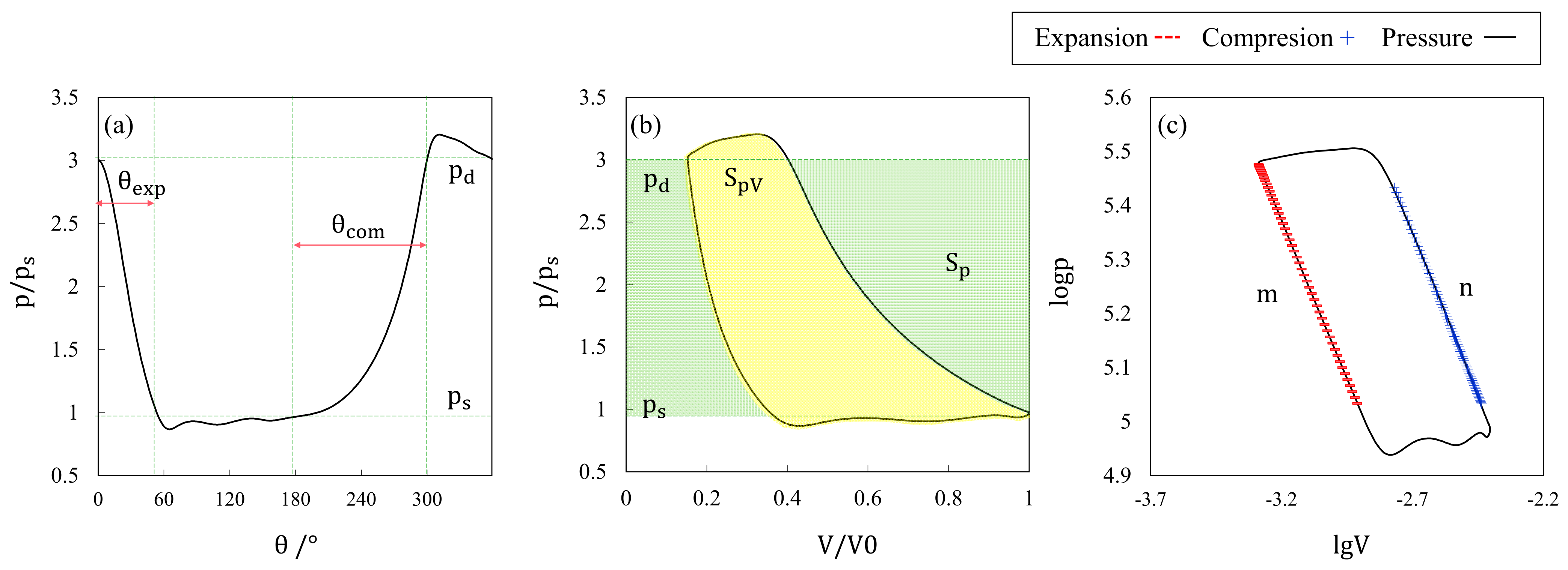
The p−V diagram describes the dynamic relationship between pressure and volume in the cylinder during a working cycle. The p−V diagram not only illustrates the indicated power from the area enclosed by the curve but also can be used to diagnose faults by comparing it to that of health conditions. Therefore, as shown in Figure 4, the following characteristic parameters are extracted from the p−θ diagram and the p−V diagram of the reciprocating compressor to form a four-dimensional feature variable:
- (1)
- Pressure ratio
- (2)
- Process angle coefficient
- (3)
- Area coefficient
- (4)
- Process parameter coefficient:
During the compression and expansion processes, the state equation of gas is [29]:
Taking the logarithm of the left and right sides of the equation to form an diagram, a linear equation with as the slope and the abscissa and ordinate as and , respectively, can be obtained as:
Then, the process parameter coefficient can be obtained by:
where is the suction pressure, is the discharge pressure, is the process angle of compression, is the process angle of expansion, is the area of the closed pressure curve in the p−V diagram, is the rectangular area enclosed by the suction pressure line and discharge pressure line, is the compression process parameter, and is the expansion process parameter.
2.2.2. Feature Extraction Based on PCA-LDA
Both Principal Component Analysis (PCA) and Linear Discriminant Analysis (LDA) are linear transformation techniques that are commonly used for dimensionality reduction [30] and data classification [31]. PCA and LDA are unsupervised and supervised learning algorithms, respectively. PCA retains the maximum amount of information while reducing the dimensionality by calculating the so-called principal components that maximize the variance in a dataset. LDA uses data labels reasonably to obtain discriminative results by computing the linear discriminants, which maximize the separation between multiple classes.
- Principal Component Analysis (PCA)
The PCA (Principal Component Analysis) method is one of the typical linear fault diagnosis methods for analyzing the covariance structure of multi-dimensional data , where is the number of variables and is the number of samples for each variable.
Firstly, the original data are standardized to be a standardized matrix The covariance matrix of a multidimensional matrix consisting of training data can be calculated as:
where , are eigenvalues and . is a feature vector. The cumulative contribution of variance (CCV) of the first principal components is obtained:
The CCV is used to estimate the extent of information retention of the newly extracted components on the original data, which is usually required to be higher than 85%, which means the following component information can be omitted, and the two principal components are sufficient to describe most of the original variable information. Eigenvectors corresponding to the first eigenvalues constitute the transformation matrix . The is a matrix of rows and columns:
The transformed data are converted by the matrix into a lower-dimensional principal component matrix:
- 2.
- Linear Discriminant Analysis (LDA)
LDA is a classification method used in statistics, pattern recognition, and other fields, to find a linear combination of features that characterizes or separates two or more classes of objects or events. For a sample of observations distributed in groups, the objective of the LDA is to produce a new representation space where we can better distinguish the groups. It uses the between-class scatter matrix to evaluate the separability of different classes and the within-class scatter matrix evaluates the compactness within each class.
First, the dataset is the training set, and each belongs to a class ().
The between-class scatter matrix is calculated as:
and the within-class scatter matrix is obtained as:
Hence, the optimization goal becomes:
where is the number of data points in class , is the center of gravity of class , and is the center of gravity of all observations.
It can be shown that the optimal vector projection is the eigenvector corresponding to the largest eigenvalues of . The projection with maximum class separability information corresponds to the eigenvectors whose eigenvalues are the highest.
The fault diagnosis result of valve leakage by the PCA-LDA method will be presented in Section 4. Integrating the advantages of PCA and LDA, the proposed method adopted in this paper is to apply PCA to extract and refine all the data as input parameters for the LDA classifier, then realize the identification and estimation of the fault severity.
3. Experiment Setup
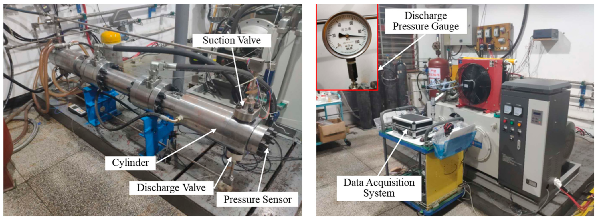
In Figure 5, a two-stage double-acting water-cooled reciprocating compressor for industrial application was modified for experimental study. It has a crank radius of 0.0575 m, a connecting rod length of 0.3 m, a cylindrical diameter of 0.195 m, a piston rod diameter of 0.035 m, and a running speed of 570 rpm. The compressor was instrumented with a data acquisition system together with several sensors recording the signals of the pressure in the cylinder, AE of valves, TDC, etc.
3.1. Measurement and Construction of the p−V Diagram
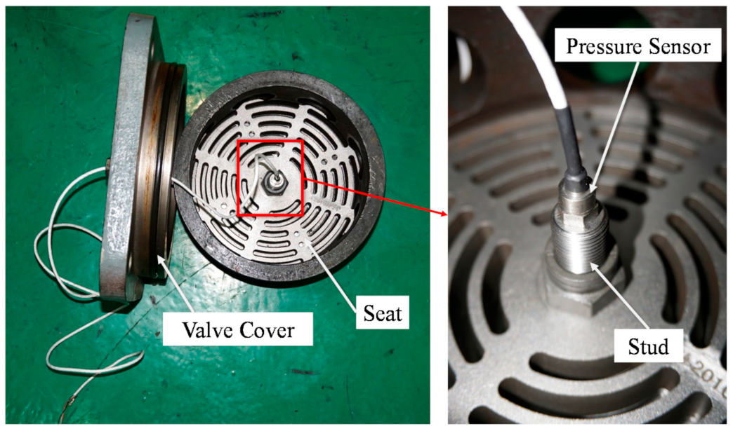
The method of acquiring the p−V diagrams in this study involved using two pressure sensors, each installed into the discharge valve studs at the crank end (CE) and head end (HE), as shown in Figure 6, to assure the actual pressures on both sides of the cylinder to be recorded instantaneously. The model of pressure sensors was XTL-190M. The overall error of the sensor was less than ±0.3% and its response frequency was as high as 10 kHz.
3.2. Experimental Mock-Up of Valve Leakage Fault
There are many reasons responsible for valve leakage, which can be mainly divided into environmental factors and mechanical factors. Environmental factors refer to the compressed medium that contains impurities, which are corrosive or improperly lubricated, causing blockage and jamming. Mechanical factors refer to the fatigue damage of the valve plate and springs caused by the irregular movement of the valve.
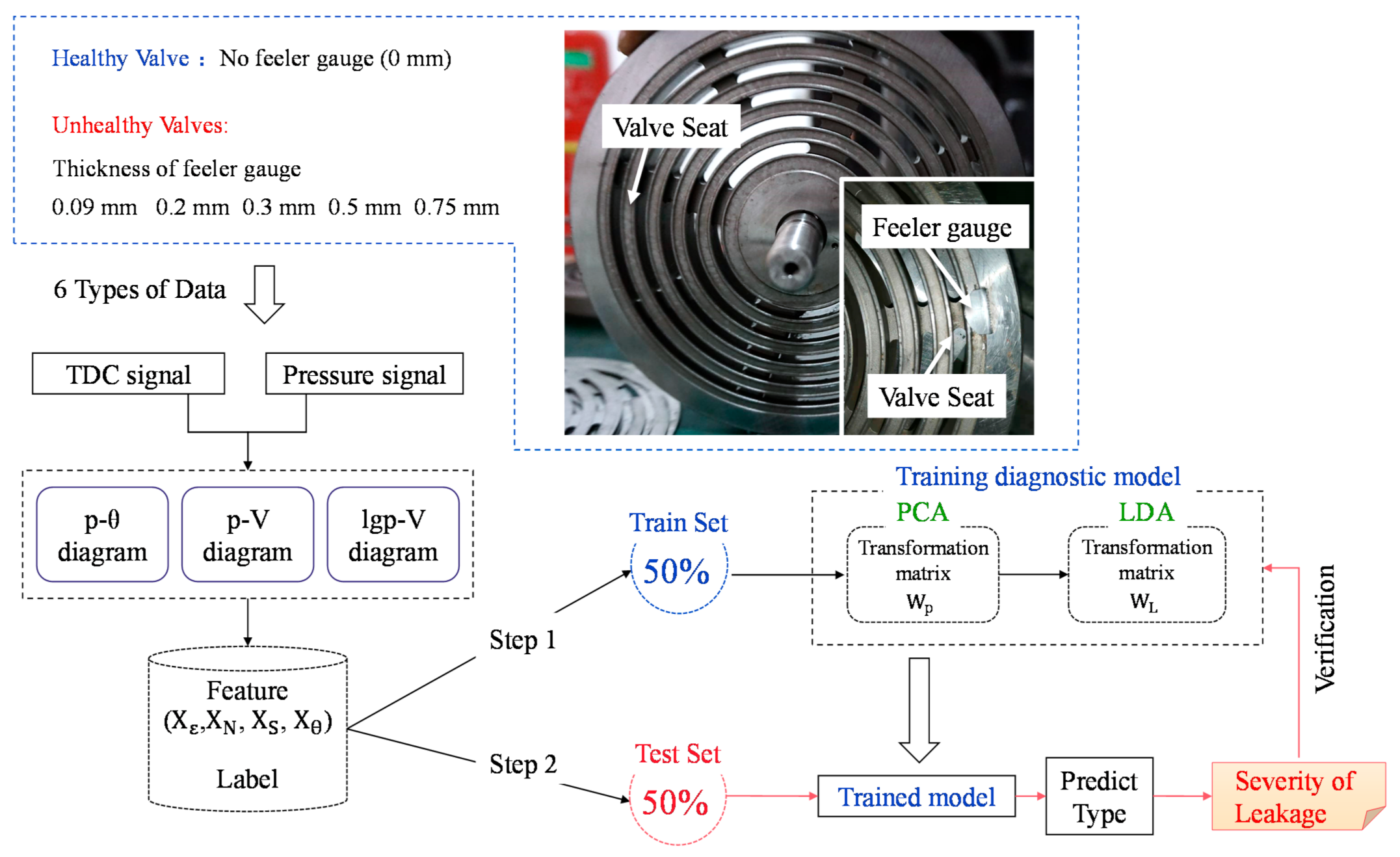
In this experiment, a feeler gauge was attached to the valve seat, so that the valve plate cannot fully fit the sealing surface of the valve seat, causing the leakage of the valve. As shown in Figure 7. The thickness of the feeler gauges selected in the comparison test in this paper was 0.09 mm, 0.2 mm, 0.3 mm, 0.5 mm, and 0.75 mm, respectively, to mock different severity of valve leakage failure.
In this paper, 2122 sets of data belonging to 6 types (1 type of healthy valve and 5 types of leakage valve) were randomly scrambled and then divided according to the ratio of 50% training set and 50% test set. The data size of specific types of data is shown in Table 1. For the judgement of the level of fault, health and mild leakage are the most easily confused and significant datasets that are needed to acquire separation. Hence, the amount of data in Type 1 and Type 2 is relatively large. Specifically, there are 365 health data and 463 mild leakage data. The characteristic variables were composed of four characteristics’ parameters (pressure ratio, process angle coefficient, p−V diagram area coefficient, and process index coefficient). Based on the training dataset, the PCA and LDA models were trained and the projection matrices and were calculated as well. Then, the test datasets were projected, and their corresponding types of faults were predicted to verify the trained model. The flow chart of the diagnosis and severity estimation method is illustrated in Figure 7.
4. Results and Discussion
4.1. Validation of the Muck-Up of Different Valve Leakage Severity
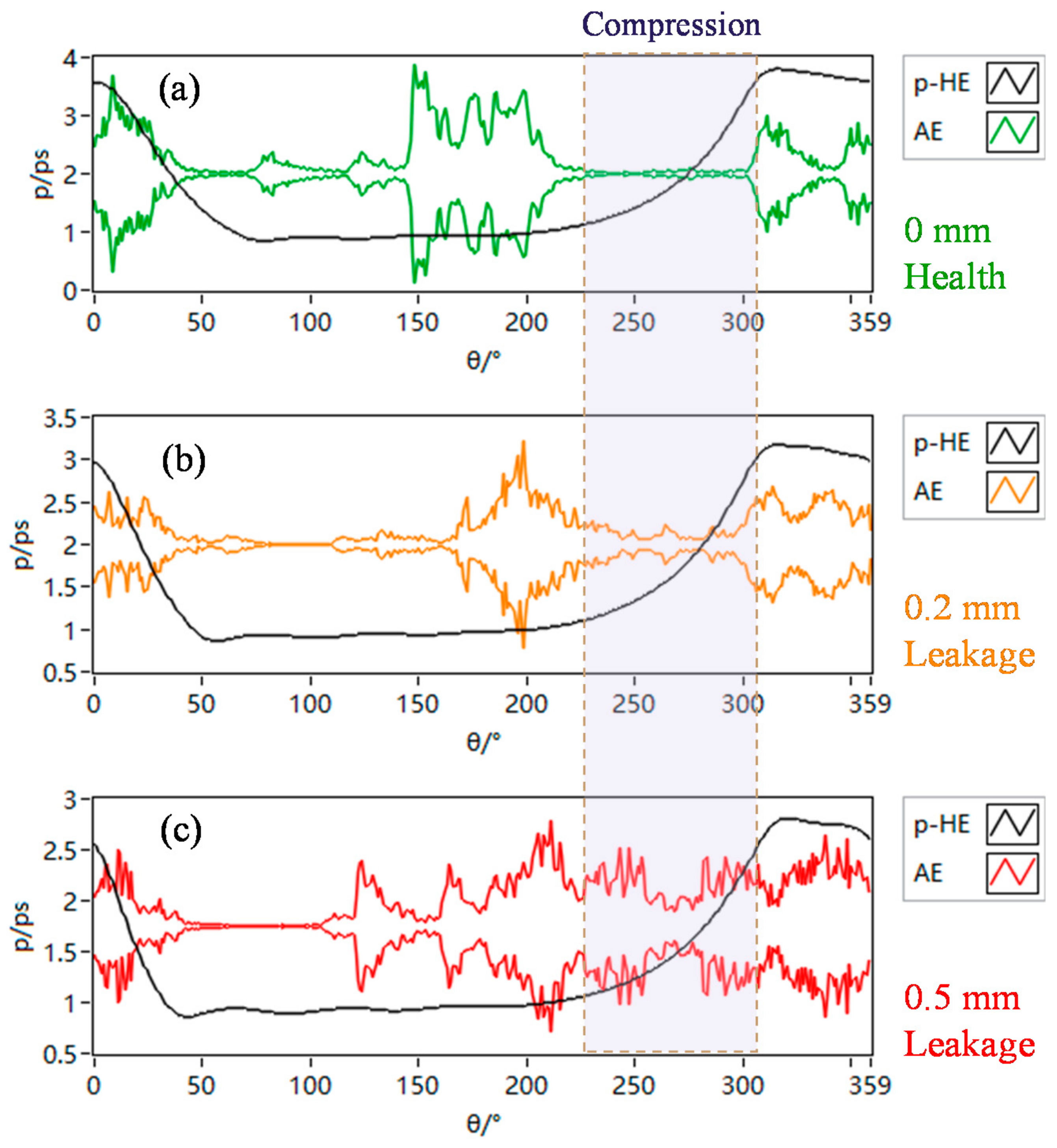
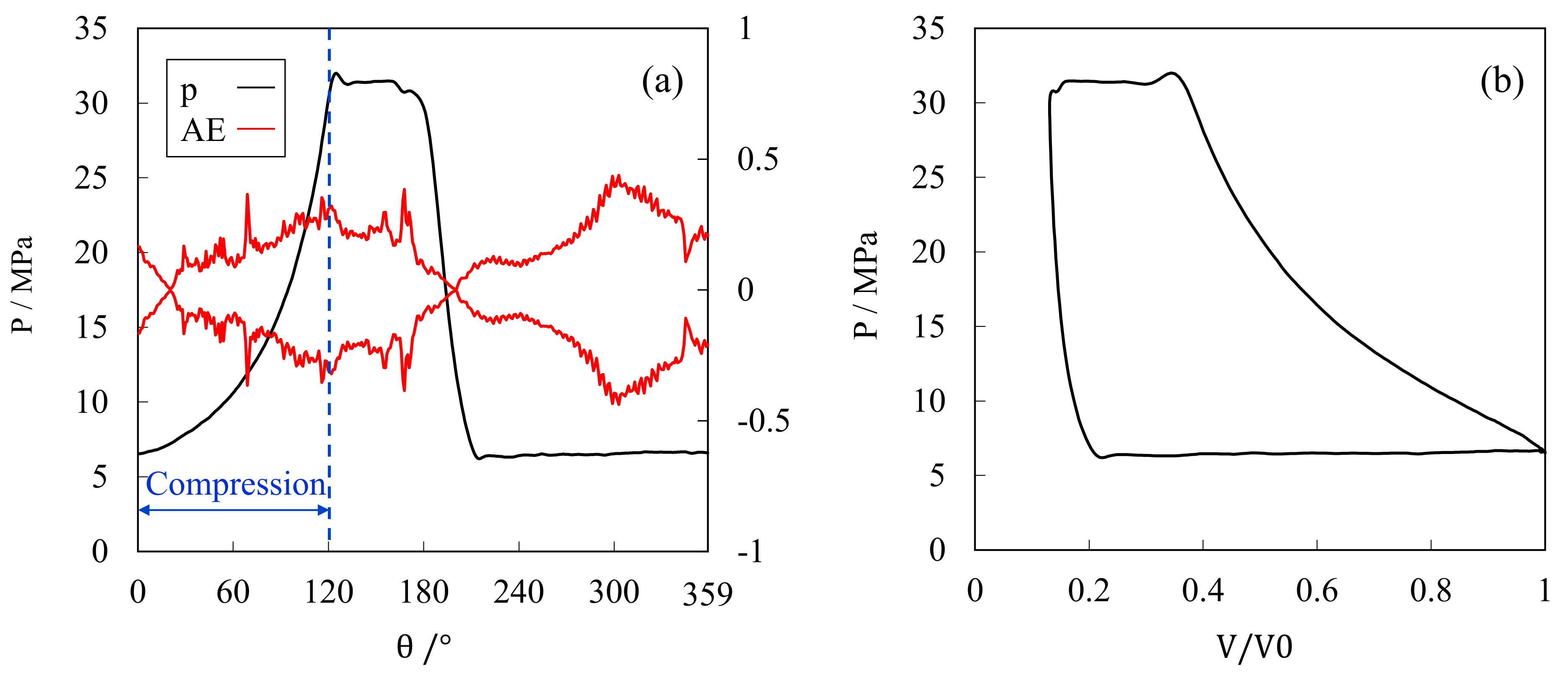
Acoustic emission (AE) technology has been used to detect valve leakage, as gas leakage can increase the peak-to-peak value of the continuous AE signal [12]. To verify the mock-up method of valve leakage by the feeler gauge, the AE signals of both the health valve (no feeler gauge, 0 mm) and leakage valve with a feeler gauge were recorded. Figure 8 shows the comparison of p−θ and AE−θ diagrams between valve leakage of different severity and health conditions. Compared to the AE signal of a health valve with no feeler gauge in Figure 8a, during the compression stroke when there should be no valve signal, a period of continuous acoustic emission signal appears in Figure 8b,c, respectively, and the amplitude of AE signals increase evidently. The above phenomenon indicates that the valve is leaking. Moreover, as the thickness of the feeler gauge increases from 0.2 mm to 0.5 mm, the leakage path of the valve becomes wider, the leakage failure becomes more serious, and the amplitude of the AE signal in the compression stroke also increases accordingly.
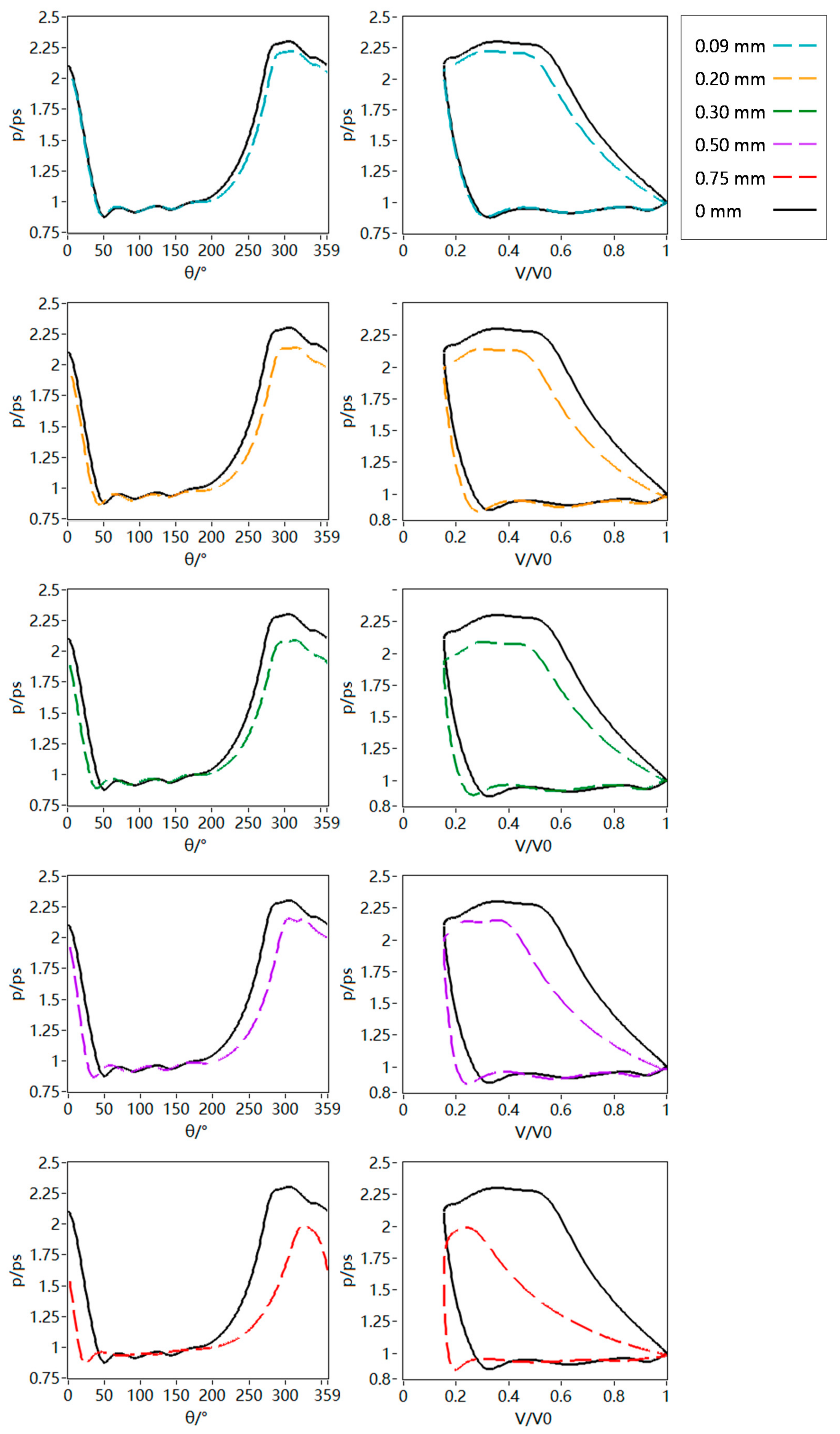
Figure 9 shows the comparison of p−θ and p−V diagrams between the valve leakage of different severity and health conditions. According to the p−V diagrams, the indicated power , compression parameter , and expansion parameter can be calculated, and the ratios of the above parameters under various leakage conditions and health conditions (,,) are shown in Table 2. It can be seen that as the severity of leakage improves (i.e., the thickness of the feeler gauge increases), the compression parameter decreases, and the expansion parameter increases. This can be explained as when there is leakage in the suction valve, during the compression process, the high-pressure gas in the cylinder will continuously leak through the suction valve from the cylinder to the suction chamber due to the pressure difference. Therefore, the piston must travel a longer stroke to improve the pressure in the cylinder to discharge pressure. Hence, the pressure rises slowly, and the compression parameter decreases. During the expansion stroke, the high-pressure gas in the cylinder will continue to leak through the suction valve as well, so as the rate of pressure drop in the cylinder rises, the corresponding stroke is shortened during the expansion process, and the expansion parameter is greatly increased.
In this paper, the loss of indicated power (i.e., the work performed by the piston on the gas) is used to measure the negative impact of leakage on the operation of the compressor. It can be seen from Table 2 that when the thickness of the feeler gauge is set to 0.09 mm, the indicated power calculated was reduced 5% compared with that of the health valve. When the feeler gauge is thickened to 0.75 mm, the indicated power is only 67% of that of the health valve, which means a loss of 33%. Based on the above analysis, we classify the severity level of the six types of fault data. The dataset without a feeler gauge (0 mm, Type 1) is classified as health. The fault level corresponding to a feeler gauge thickness of 0.09 mm (Type 2) is mild leakage. The fault level corresponding to a feeler gauge thickness of 0.2 mm, 0.3 mm, and 0.5 mm (Types 3, 4, 5) belongs to moderate leakage, and a 0.75-mm-thick feeler gauge (Type 6) corresponds to serious leakage.
4.2. Feature Parameter Analysis
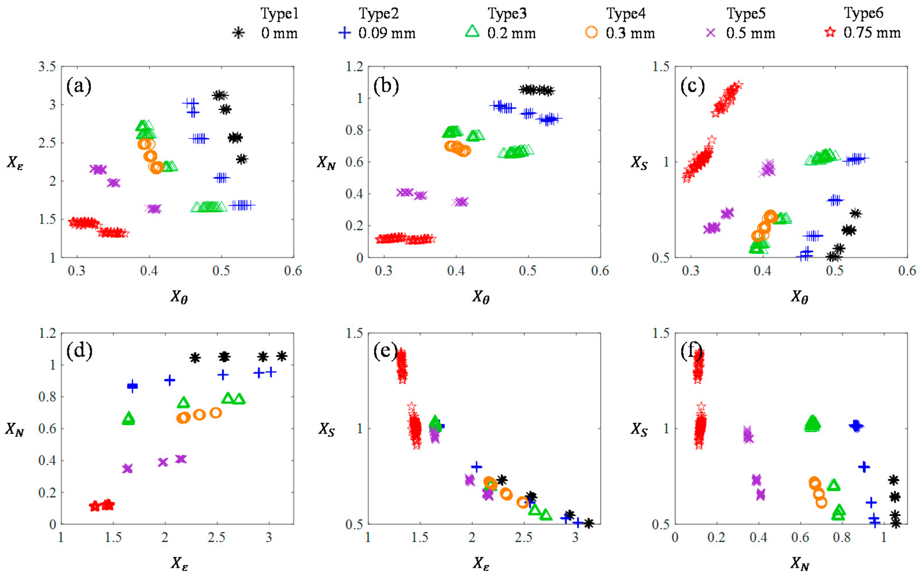
The four characteristic variables extracted from the training dataset p−V diagram are arranged and combined as the horizontal and vertical coordinates, and training sets of data are projected in a two-dimensional space, as shown in Figure 10. Data points show relatively obvious linear separability in two-dimensional space as the level of failure changes, which indicates the selected features can reflect the characteristics of the p−V diagram. It can be observed that data points of the serious leakage (i.e., the thickness of the feeler gauge is 0.75 mm, red data points) have a large difference from the other types in the 2D diagrams. In Figure 10b,d,f, from a one-dimensional perspective of the process index coefficient , different types of data show the greatest separation, which means it contributes to fault identification to a great extent. In Figure 10e, the same kind of failure data points show a relatively lower concentration, and the data points of Type 1–5 aliased together in the 2D space of the area coefficient and the pressure ratio coefficient. It illustrates that although these two features respond to fault variety, they cannot play major roles in distinguishing fault. It is worth noting that, in Figure 10a–c, the process angle coefficient can cause all types of data to be evenly distributed, but the concentration of the same type of data is not satisfactory, and the overlapping ranges of two adjacent datasets are considerable.
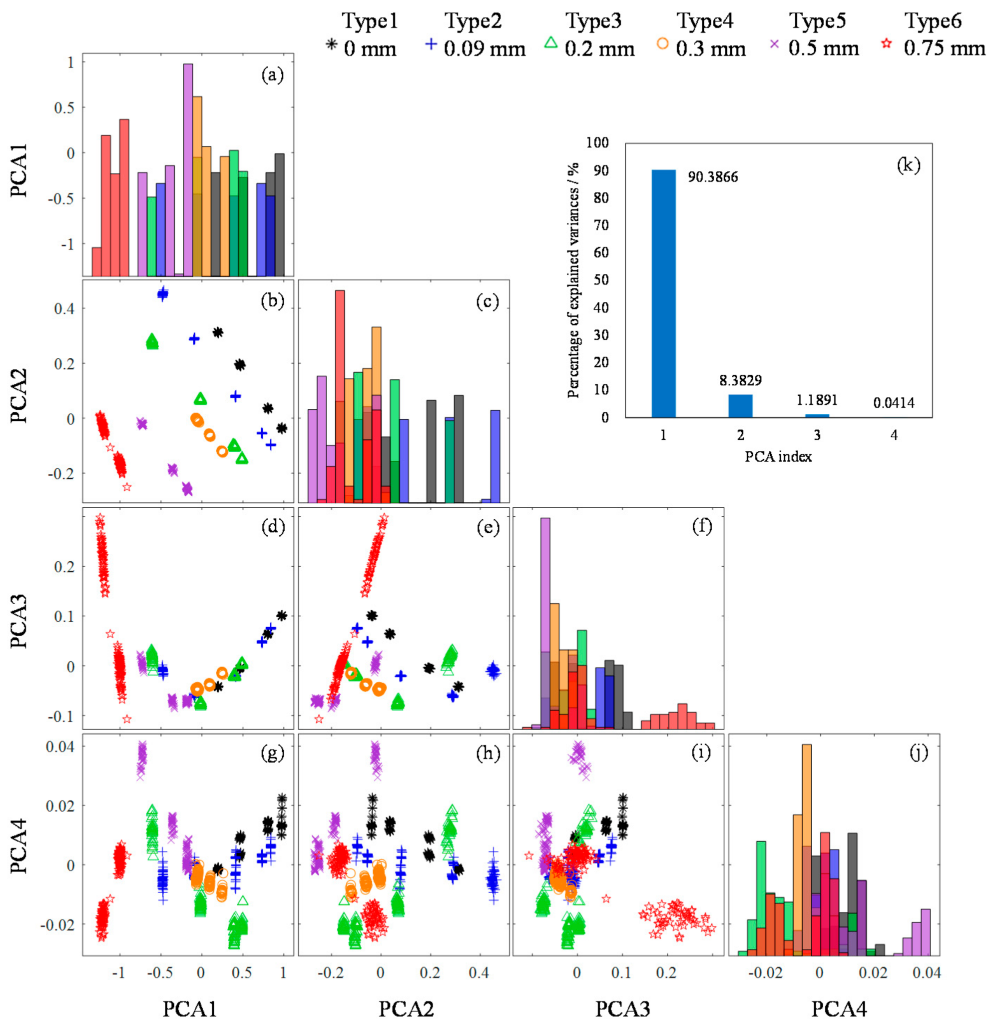
From the left diagonal of the matrix diagram (in Figure 11), the data histogram reflects the distribution of the data from the first to the fourth principal component, which varies from clear to complex. In the direction of the first principal component, health and serious fault data points (red and black data points) are completely separated. The one-dimensional histogram of the first principal component shows that there are more overlapping areas, and data distribution ranges of 0.09–0.5 mm feeler gauges cannot be distinguished. This means that PCA did not achieve satisfactory classification results but did amplify and extract the preliminary features. That can be explained by the fact that PCA is an unsupervised algorithm with no category information. It selected the direction with the largest variance of the whole training data after projection, and more information can be illustrated by the larger variance amplitude. So, the PCA method based on the maximum variance of the overall data and ignoring the data category did not perform well in the classification of mild and moderate faults. However, it still can be noted that data groups have already presented a linear distribution basically in the light of type in the 2D space formed by PCA1 and PCA2 (with the component score for PCA1 and PCA2 being 98.77%). Therefore, another projection is needed to pursue more accurate data classification.
Next, the PCA transformed data were utilized as LDA input parameters. After LDA, from the two-dimensional space observation in Figure 12, the distribution result of different types of faults was more distinct than that after PCA. Especially, the percentage of explained variances of the first projection direction reaches more than 99%. Besides, the obvious overlapping areas were no longer shown on the histogram of various types of data. What is more, the data groups present a unidirectional linear distribution according to the level of failure in the direction of LDA1. This means that the information of the p−V diagram was successfully reduced to one dimension, and the distribution result of different types of faults was more distinct than that after PCA, which is enough to conduct a determination of the level of leakage fault. The above analysis confirmed the necessity and effectiveness of LDA.
4.3. Comparisons with Other Methods
In this section, the other four established data dimensionality reduction methods were utilized to process the data of the test set, including t-Distributed Stochastic Neighbor Embedding (TSNE), Kernel Principal Component Analysis (KPCA), Locality Preserving Projections (LPP), and a Support Vector Machine (SVM).
T-Distributed Stochastic Neighbor Embedding (t-SNE) [32] is a dimensionality reduction technique used to represent high-dimensional datasets in a two-dimensional or three-dimensional low-dimensional space to visualize them. T-SNE creates a reduced feature space, wherein similar samples are modelled by nearby points and dis-similar samples are modelled by high-probability distant points. Principal Components Analysis (PCA) is suitable for linear dimensionality reduction of data. Kernel Principal Component Analysis [33] (KPCA) can realize non-linear dimensionality reduction of data and is used to process linearly inseparable datasets. For data with high-order correlations, Kernel Principal Component Analysis (KPCA) can realize non-linear dimensionality reduction of data and is used to process linearly inseparable data sets. For data with high-order correlations, the sample data are mapped to high-dimensional data, and then the linear classifier PCA is used to reduce the dimensionality, so as to realize the classification of non-linear data. LPP [34] is a linear technique, which projects data in the direction of maximum variance. When the high-dimensional data lay on the low-dimensional manifold embedded in the ambient space, the LPP is realized by finding the best linear approximation of the eigenfunctions of the Laplacian Beltrami operator on the manifold. SVM [35] is used for fault classification due to its superiority in dealing with small sample problems, which can guarantee the local and globally optimal solutions are exactly the same.
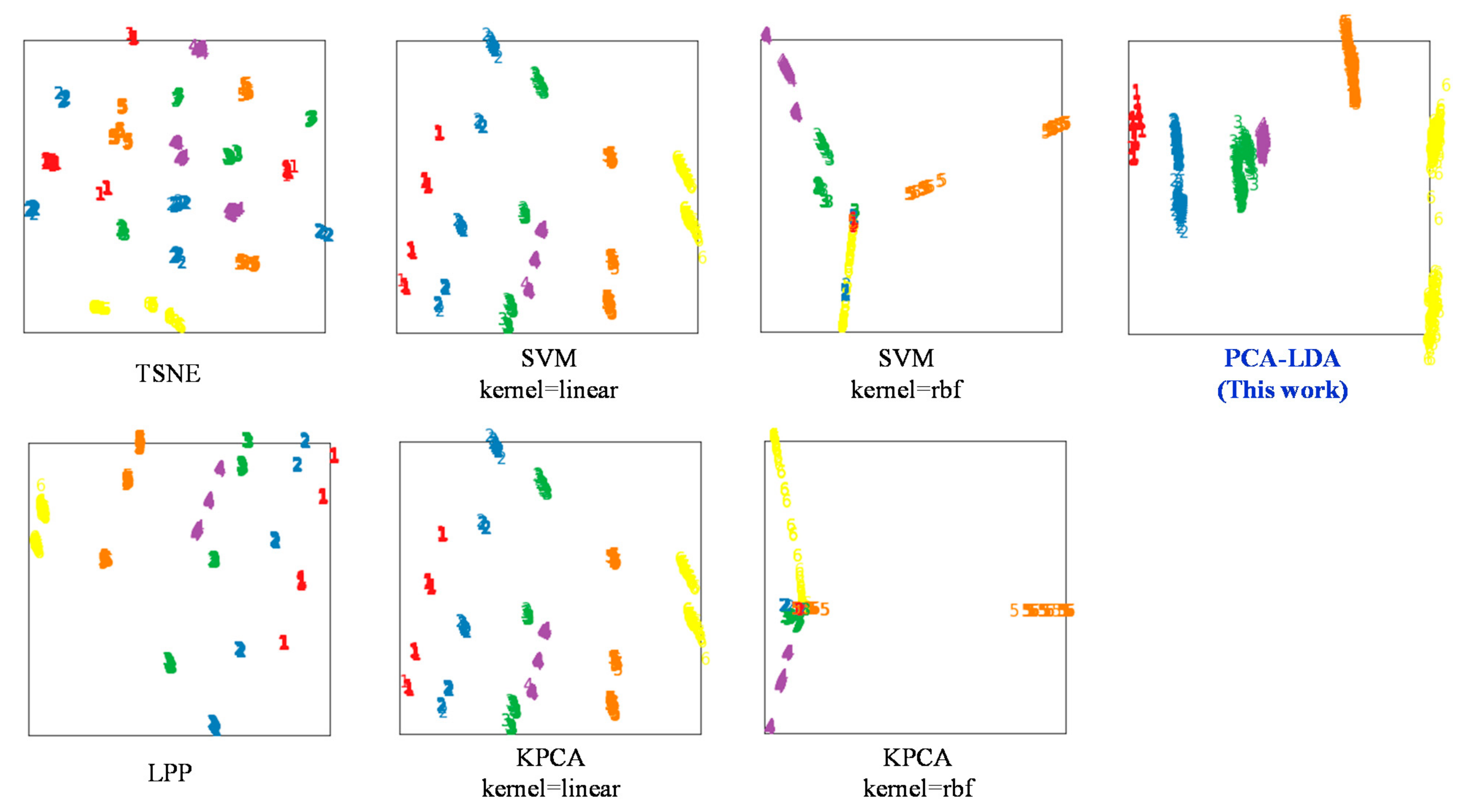
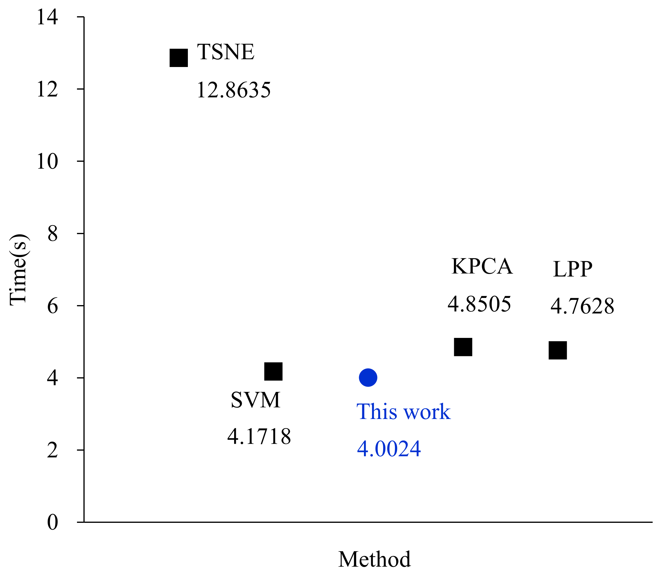
Figure 13 and Figure 14 show the comparison between the 2D projection and calculation time of the above methods and that of this work. The TSNE distribution shows that the same type of fault data are scattered and aggregated, that is, the same type of fault data may be gathered in multiple locations, and the distribution of data points is chaotic and does not achieve the desired classification effect. The computational cost of t-SNE is very high with large memory and long-duration running time as well. In Figure 10, the data present a linearly separable characteristic in 2D space. Hence, when moving on to the projection of KPCA and SVM, the analysis result of adopting the linear kernel is significantly better than the RBF kernel. When using the RBF kernel, they cannot distinguish the distribution of various kinds of data. The data of Type 1, Type 2, Type 3, and Type 6 are mixed together while that of Type 4 and Type 5 realize a relatively better differentiation and aggregation effect, which is not satisfactory enough either. When using the linear kernel, the results of the two methods are highly consistent. The result of LPP, another linear method, is very close to that of SVM and KPCA, and the data have shown fair separation and linear distribution tendency. However, from a one-dimensional perspective, the degree of aggregation of LPP in a one-dimensional direction is not as good as that of SVM and KPCA. As to the method proposed in this paper, it is obviously superior to use the method based on PCA-LDA. The data points of the same type show a high level of compactness on one dimension, and the distinctions between various types are farther. Besides, Figure 14 illustrates the comparison of the calculation time of each method. The shortest time consumed further confirms the high efficiency and effectiveness of this work.
4.4. Severity Estimation of Valve Leakage
According to the above analysis, the method of feature extraction of the p−V diagram and the severity estimation of the valve leakage fault can be concluded. First, the pressure ratio coefficient, process angle coefficient, area coefficient, and process index coefficient of the p−V diagram are extracted to form the four-dimensional feature variables. The PCA algorithm is used to amplify and extract the preliminary features of the data to obtain the projection matrix . Then, the PCA transformed data are utilized as LDA input parameters to calculate the projection matrix , and the classifier training is complete. Next, the trained diagnostic model is used to predict the fault type of the test dataset. Figure 15 shows the confusion matrix of the predicted result. It shows that four data points attributable to 0.2 mm are incorrectly predicted to be 0.3 mm. In addition to this, the prediction results of other test data points are correct. The overall recognition accuracy reaches 99.62%.
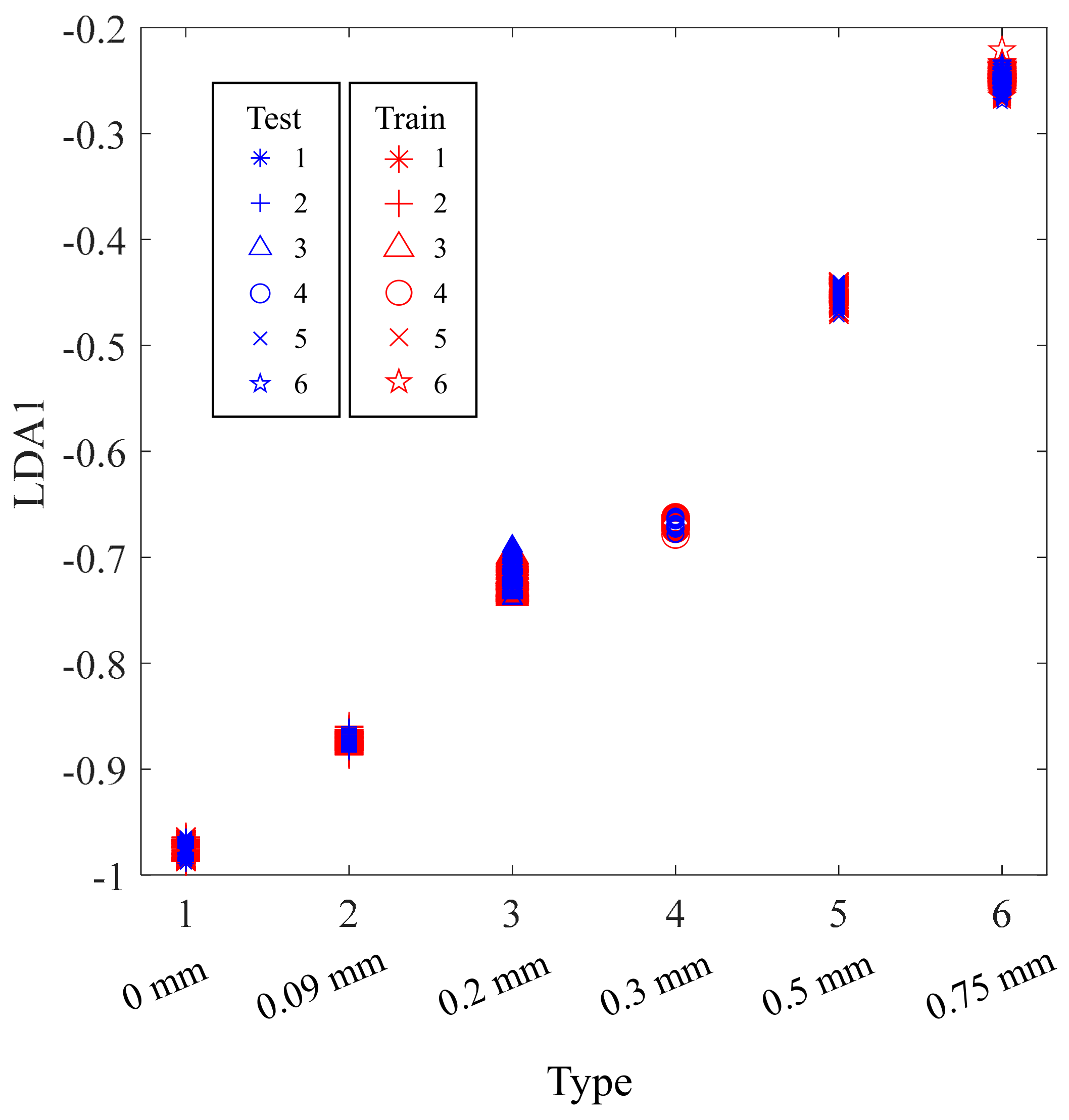
In Figure 16, the test set and the training set are projected in the direction of LDA1, wherein the data points of the same type show a high level of compactness, and the distinctions between various types are obvious. Besides, the data between the test set and the training set overlap to a great extent as well. It is undeniable that the distance between data points of type 2 (0.2 mm) and type 3 (0.3 mm) is close, where error is also generated. However, the difference of indicated power loss caused by the above two leakage faults is also very close (8% and 9%), and both belong to moderate leakage faults. Therefore, the above error is considered acceptable.
4.5. Fault Diagnosis of Valves
4.5.1. Application in the Mild Leakage Caused by the Cracked Valve Plate
Figure 17 shows the p–V diagram of a fault condition in which the suction pressure was 88 kPa and discharge pressure is 343 kPa. After being converted by the projection matrix , obtained from the above training, the predicted result was type 2, which represented mild leakage of the valve. In addition to the environmental factors such as impurities entrapped by the compressed gas, the mechanical factor is also one of the unignorable reasons for the mild leakage. The mechanical factor mainly refers to valve damage caused by high cycle fatigue or irregular valve motion [36]. During the operation of the compressor, especially the compressor with a high rotation speed, the valve plate is constantly subjected to high-frequency shocks caused by hitting the valve seat and limiter. Cracks or breakage in the valve plate can result in leakage failure, and in turn, the mild leakage may indicate an early crack fault.
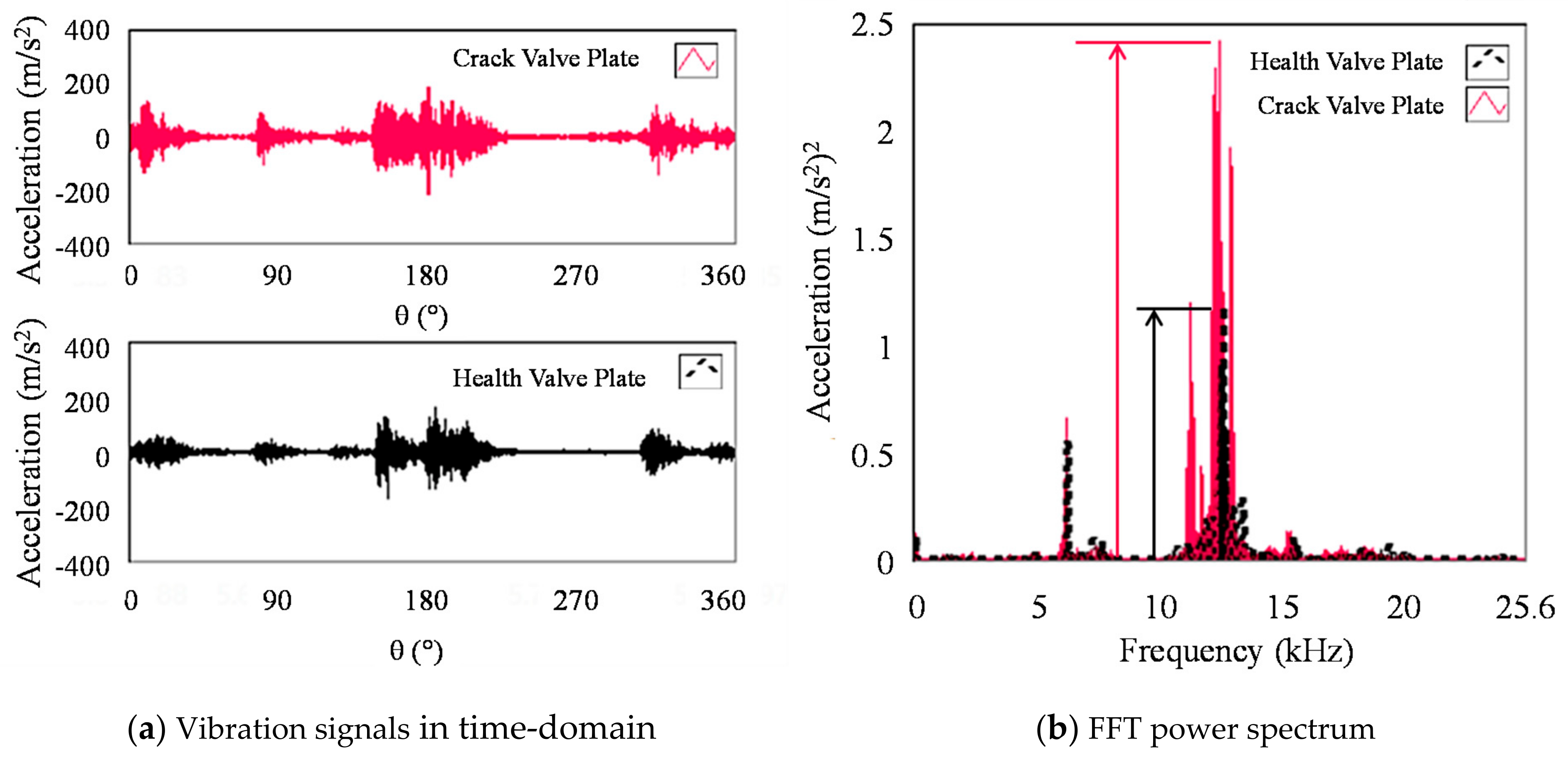
Hence, the vibration signal was integrated to validate the judgment above, and further determine the reason for the leakage comprehensively. The crack or local defect affects the dynamic response of a structural member, which can be detected by vibration measurement [37]. Considering the transient characteristics of the event of impact between the valve plate and valve seat, the occurrence of cracks induced the change of valve plate stiffness. Therefore, when the valve plate hit the valve seat and limiter, the time-domain amplitude and frequency-domain energy distribution of the vibration signal changed significantly. Figure 18 illustrates the comparison of the FFT power spectrums between the vibration signal from the health valve and the cracked valve. It can be seen that, in the range of the 10–15 kHz high-frequency band, the amplitude of the power spectrum undergoes a significant increase (i.e., the red line compared to the black line), which means the measured component indicates the existence of a crack fault.
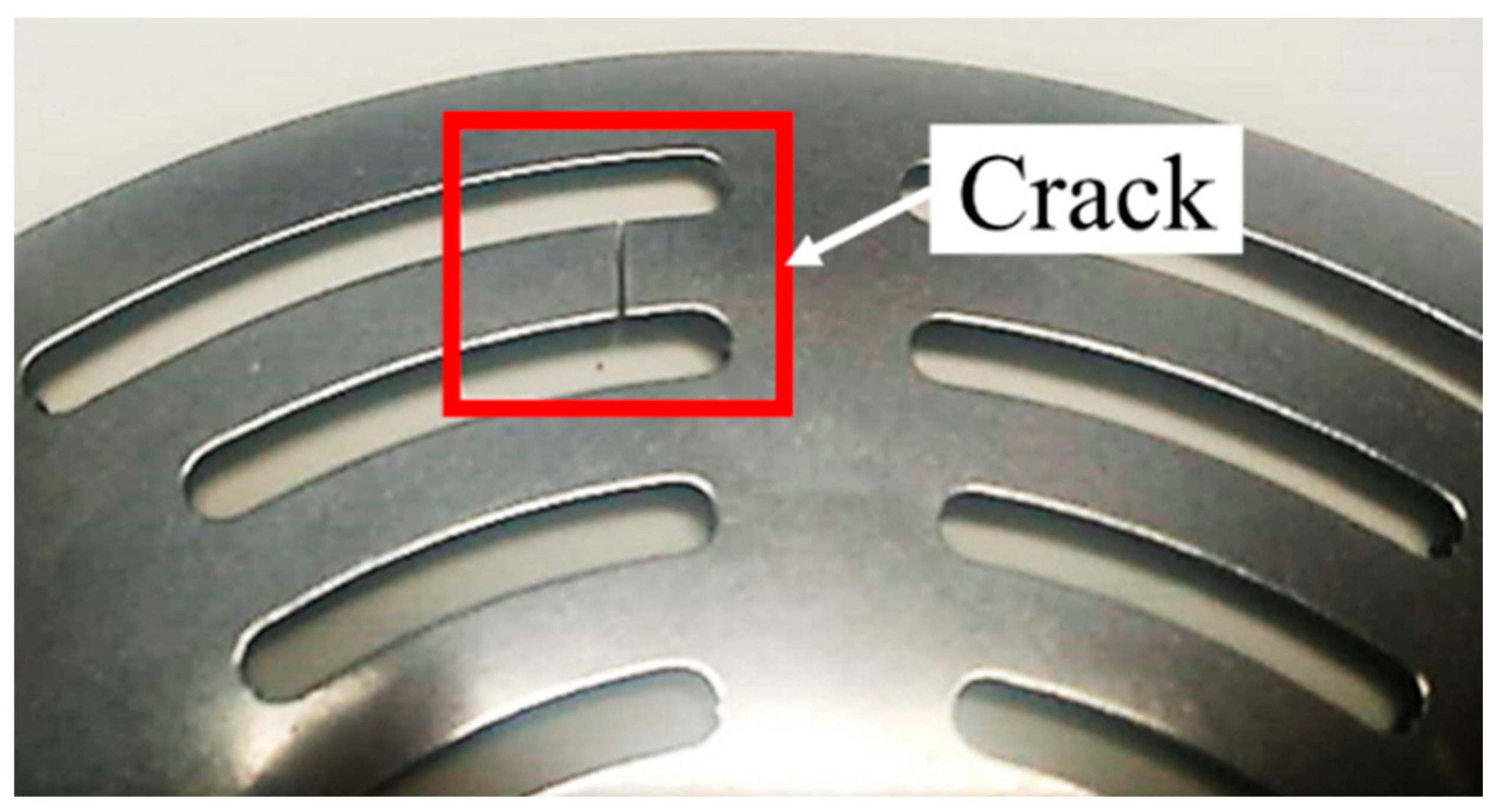
In Figure 19, there was a thorough crack on the valve plate, which led to the mild leakage of the valve. Therefore, the method proposed in this paper realized the diagnosis of the mild leakage failure caused by a cracked valve plate in the reciprocating compressor.
4.5.2. Application in the Serious Leakage Caused by the Deformed Valve Plate
The proposed method was also applied in the valve of the hydraulically driven piston compressor [38], which is another kind of reciprocating compressor designed to com-press hydrogen to 90 MPa for HRSs, as shown in Figure 20. The pressure sensor was in-stalled through the cylinder end cover to record the p−V diagram.
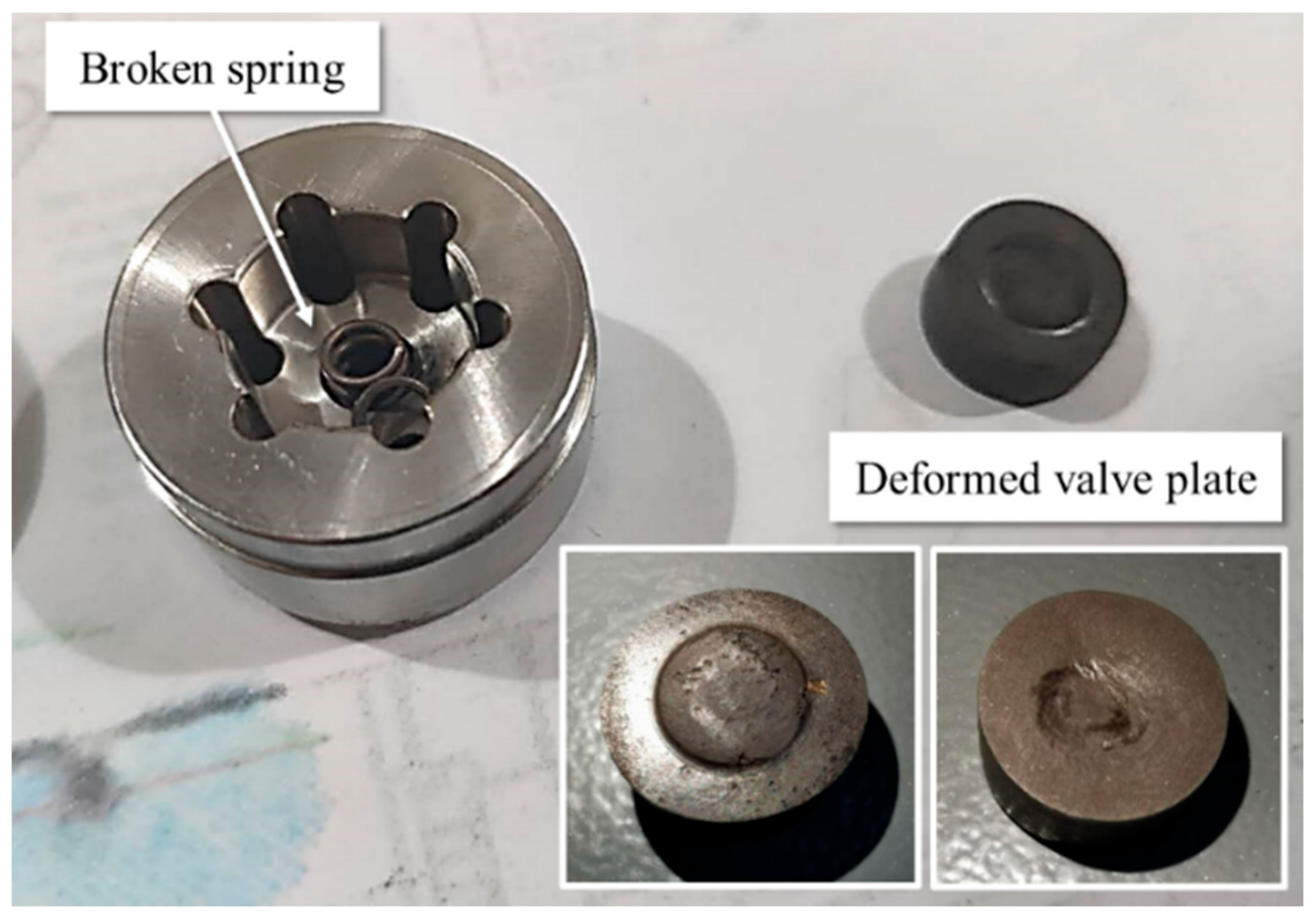
In the fault condition, Figure 21 indicates the suction pressure was 6.2 MPa, discharge pressure was 30.8 MPa. The compressor operated at 16 cycles per minute. While the unit was operating, the temperature of the suction line increased abnormally, and the feature was extracted from the p−V diagram in Figure 21b to diagnose and estimate the fault severity. The obtained result was Type 4, which was the fault severity range of moderate leakage. On the other hand, the AE signal was also monitored on the valve cover, which indicated valve leakage because of the increased peak-to-peak value of the continuous AE signal during compression period, shown by the red line in Figure 21a.
After disassembling and inspecting the valve of the compressor, it was found the valve spring was broken, and the central area of the valve plate was severely deformed, causing the failure of the sealing surface of the valve, as shown in Figure 22. Therefore, the diagnosis acquired an accurate and satisfactory result.
Then, the broken valve spring and deformed valve plate were replaced. In the operation condition of the suction pressure at 1.6 MPa and discharge pressure at 7.8 MPa, the compressor operated at 16 cycles per minute. The result of identification became the health (Type 0). The pressure in the cylinder and AE signal of the valve indicated that the leakage was repaired, for the reason that, during the compression and expansion period, there was no apparent continuous AE signal with increasing amplitude (in Figure 23).
5. Conclusions
In this paper, fault identification of a reciprocating compressor valve employing features of the p−V diagram and linear discrimination analysis is proposed, which was further validated by the diagnosis of different severities of valve leakage, and the fault diagnosis of the reciprocating compressor valve in a hydraulically driven piston compressor for HRSs. Several conclusions are drawn:
- (1)
- Four-dimensional variables composed of the pressure ratio, process angle coefficient, p−V area coefficient, and process index coefficient can be extracted from the p−V diagram to serve as the characteristics to illustrate the severity of the failure. The process index coefficient contributes to fault identification to great extent.
- (2)
- The PCA can be used to amplify and extract the preliminary features of the characteristic variables and separate the data of serious leakage faults, and the PCA-projected dataset was employed as the input parameter to the LDA classifier to achieve an optimized classification result.
- (3)
- The diagnosis and identification results of various fault data show good consistency with the actual faults including the cracked valve plate and the deformed valve in the application on the reciprocating compressor and the hydraulically driven piston compressor.
- (4)
- This finding indicates the p−V diagram-based method as an effective diagnosis tool for self-acting valve failure, which would have great potential in many application scenarios, including gas storage, hydrogen refueling station, etc.
Author Contributions
Conceptualization: X.P. and Z.Z.; methodology: X.L. and P.R.; software: X.L.; validation: X.L. and P.R.; writing—original draft preparation, X.L.; writing—review and editing, X.P. and X.J.; visualization: X.L. and Z.Z.; supervision: Z.Z.; project administration: X.P. and X.J. All authors have read and agreed to the published version of the manuscript.
Funding
This work was supported by the National Natural Science Foundation of China through grant No. 51876155.
Institutional Review Board Statement
Not applicable.
Informed Consent Statement
Not applicable.
Data Availability Statement
Data used to support the findings of this study may be available from the corresponding author upon request, subject to compliance with the relevant data protection laws and regulations.
Conflicts of Interest
The authors declare no conflict of interest.
References
- Giorgetti, S.; Giorgetti, A.; Jahromi, R.T.; Arcidiacono, G. Machinery Foundations Dynamical Analysis: A Case Study on Reciprocating Compressor Foundation. Machines 2021, 9, 228. [Google Scholar] [CrossRef]
- PROGNOST. PROGNOST Systems GmbH Company Profile. Available online: https://www.prognost.com/2016/07/28/compressor-valve-monitoring/ (accessed on 7 December 2021).
- Loukopoulos, P.; Zolkiewski, G.; Bennett, I.; Sampath, S.; Pilidis, P.; Li, X.; Mba, D. Abrupt fault remaining useful life estimation using measurements from a reciprocating compressor valve failure. Mech. Syst. Signal Process. 2019, 121, 359–372. [Google Scholar] [CrossRef]
- Kolodziej, J.R.; Trout, J.N. An image-based pattern recognition approach to condition monitoring of reciprocating compressor valves. J. Vib. Control 2017, 24, 4433–4448. [Google Scholar] [CrossRef]
- Zhao, B.; Jia, X.; Sun, S.; Wen, J.; Peng, X. FSI model of valve motion and pressure pulsation for investigating thermodynamic process and internal flow inside a reciprocating compressor. Appl. Therm. Eng. 2018, 131, 998–1007. [Google Scholar] [CrossRef]
- Sharma, V.; Parey, A. Performance evaluation of decomposition methods to diagnose leakage in a reciprocating compressor under limited speed variation. Mech. Syst. Signal Process. 2018, 125, 275–287. [Google Scholar] [CrossRef]
- Zhou, D.; Huang, D.; Hao, J.; Ren, Y.; Jiang, P.; Jia, X. Vibration-based fault diagnosis of the natural gas compressor using adaptive stochastic resonance realized by Generative Adversarial Networks. Eng. Fail. Anal. 2020, 116, 104759. [Google Scholar] [CrossRef]
- Liang, Z.; Li, S.; Tian, J.; Zhang, L.; Feng, C.; Zhang, L. Vibration cause analysis and elimination of reciprocating compressor inlet pipelines. Eng. Fail. Anal. 2015, 48, 272–282. [Google Scholar] [CrossRef]
- Townsend, J.; Badar, M.A.; Szekerces, J. Updating temperature monitoring on reciprocating compressor connecting rods to improve reliability. Eng. Sci. Technol. Int. J. 2016, 19, 566–573. [Google Scholar] [CrossRef] [Green Version]
- Becerra, J.A.; Jimenez, F.J.; Torres, M.; Sanchez, D.T.; Carvajal, E. Failure analysis of reciprocating compressor crankshafts. Eng. Fail. Anal. 2011, 18, 735–746. [Google Scholar] [CrossRef]
- El-Ghamry, M.; Reuben, R.; Steel, J. The Development of Automated Pattern Recognition and Statistical Feature Isolation Techniques for the Diagnosis of Reciprocating Machinery Faults Using Acoustic Emission. Mech. Syst. Signal Process. 2003, 17, 805–823. [Google Scholar] [CrossRef]
- Wang, Y.; Xue, C.; Jia, X.; Peng, X. Fault diagnosis of reciprocating compressor valve with the method integrating acoustic emission signal and simulated valve motion. Mech. Syst. Signal Process. 2015, 56–57, 197–212. [Google Scholar] [CrossRef]
- Chlumsky, V. Reciprocating and Rotary Compressors; SNTL-Publisher of Technical Literature: Prague, Czechoslovakia, 1965; pp. 502–506. [Google Scholar]
- Manepatil, S.S.; Tiwari, A. Fault Diagnosis of Reciprocating Compressor Using Pressure Pulsations. In Proceedings of the International Compressor Engineering Conference, West Lafayette, IN, USA, 9–12 July 2018. [Google Scholar]
- Elhaj, M.; Almrabet, M.; Rgeai, M.; Ehtiwesh, I. A combined practical approach to condition monitoring of reciprocating compressor using IAS and dynamic pressure. World Acad. Sci. Eng. Technol. 2010, 63, 186–192. [Google Scholar]
- Real, M.; Pereira, E. Measuring Hermetic Compressor Valve Lift Using Fiberoptic Sensors. In Proceedings of the 7th IIR International Conference on Compressors and Coolants, Castá Papiernicka, Slovak, 30 September–2 October 2009. [Google Scholar]
- Kim, J.; Wang, S.; Park, S.; Ryu, K.; La, J. Valve Dynamic Analysis of a Hermetic Reciprocating Compressor. In Proceedings of the International Compressor Engineering Conference, West Lafayette, IN, USA, 17–20 July 2006. [Google Scholar]
- Li, X.; Peng, X.; Zhang, Z.; Jia, X.; Wang, Z. A new method for nondestructive fault diagnosis of reciprocating compressor by means of strain-based p–V diagram. Mech. Syst. Signal Process. 2019, 133, 106268. [Google Scholar] [CrossRef]
- Windrock. Windrock 6400 Portable Analyzer. 2020. Available online: https://windrock.com/wp-content/uploads/2019/06/Windrock-6400-Brochure_060319_sm.pdf (accessed on 7 December 2021).
- HOERBIGER (Shanghai) Co. Ltd. Reciprocating Compressor Condition Monitoring. 2014. Available online: https://www.utilityengineers.net/specialist/Conditioning%20Monitoring.pdf (accessed on 7 December 2021).
- PROGNOST. Evaluating the Strengths and Weaknesses of the Most Common Online Condition Monitoring Technologiesm. 2014. Available online: https://www.prognost.com/wp-content/uploads/2018/03/ct2-06-14_compressor-valve-monitoring.pdf (accessed on 7 December 2021).
- Bently Nevada. OptiComp™ BN Compressor Control Suite. 2015. Available online: https://www.bakerhughesds.com/sites/g/files/cozyhq596/files/acquiadam_assets/gea30389a_opticompbrochure_printed_r2.pdf (accessed on 7 December 2021).
- Ahmed, M.; Baqqar, M.; Gu, F.; Ball, A.D. Fault Detection and Diagnosis Using Principal Component Analysis of Vibration Data from A Reciprocating Compressor. In Proceedings of the 2012 UKACC International Conference on Control, Cardiff, UK, 3–5 September 2012; pp. 461–466. [Google Scholar] [CrossRef] [Green Version]
- Wang, Y.; Wu, D.; Yuan, X. LDA-based deep transfer learning for fault diagnosis in industrial chemical processes. Comput. Chem. Eng. 2020, 140, 106964. [Google Scholar] [CrossRef]
- Wang, F.; Song, L.; Zhang, L.; Li, H. Fault Diagnosis for Reciprocating Air Compressor Valve Using P−V Indicator Diagram and SVM. In Proceedings of the 3rd International Symposium on Information Science and Engineering, Shanghai, China, 24–26 December 2010; pp. 255–258. [Google Scholar] [CrossRef]
- Feng, K.; Jiang, Z.; He, W.; Ma, B. A recognition and novelty detection approach based on Curvelet transform, nonlinear PCA and SVM with application to indicator diagram diagnosis. Expert Syst. Appl. 2011, 38, 12721–12729. [Google Scholar] [CrossRef]
- Pichler, K.; Lughofer, E.; Pichler, M.; Buchegger, T.; Klement, E.; Huschenbett, M. Detecting broken reciprocating compressor valves in the PV diagram. In Proceedings of the IEEE/ASME International Conference on Advanced Intelligent Mechatronics, Wollongong, NSW, Australia, 9–12 July 2013; pp. 1625–1630. [Google Scholar]
- Hanlon, P.C. Compressor Handbook; McGraw-Hill: New York, NY, USA, 2001. [Google Scholar]
- Shen, W.D.; Tong, J.G. Thermodynamics of Engineering; Higher Education Press: Beijing, China, 2007; pp. 267–269. [Google Scholar]
- Zhang, Y.; Xu, T.; Chen, C.; Wang, G.; Zhang, Z.; Xiao, T. A hierarchical method based on improved deep forest and case-based reasoning for railway turnout fault diagnosis. Eng. Fail. Anal. 2021, 127, 105446. [Google Scholar] [CrossRef]
- Kim, H.; Drake, B.L.; Park, H. Multiclass classifiers based on dimension reduction with generalized LDA. Pattern Recognit. 2007, 40, 2939–2945. [Google Scholar] [CrossRef] [Green Version]
- Chen, J.; Zhou, D.; Lyu, C.; Lu, C. Feature reconstruction based on t-SNE: An approach for fault diagnosis of rotating machinery. J. Vibroeng. 2017, 19, 5047–5060. [Google Scholar] [CrossRef] [Green Version]
- Pilario, K.E.; Shafiee, M.; Cao, Y.; Lao, L.; Yang, S.H. A review of kernel methods for feature extraction in nonlinear process monitoring. Processes 2020, 8, 24. [Google Scholar] [CrossRef] [Green Version]
- He, X.; Niyogi, P. Locality Preserving Projections. Proc. Adv. Neural Inf. Process. Syst. 2003, 16, 153–160. [Google Scholar]
- Yang, Y.; Yu, D.; Cheng, J. A fault diagnosis approach for roller bearing based on IMF envelope spectrum and SVM. Measurement 2007, 40, 943–950. [Google Scholar] [CrossRef]
- Brun, K.; Nored, M.G.; Gernentz, R.S.; Platt, J.P. Reciprocating Compressor Valve Plate Life and Performance Analysis. In Proceedings of the Gas Machinery Conference, Covington, LA, USA, 3–5 October 2005; pp. 1–15. [Google Scholar]
- Bovsunovsky, A.P. Efficiency analysis of vibration based crack diagnostics in rotating shafts. Eng. Fract. Mech. 2017, 173, 118–129. [Google Scholar] [CrossRef]
- Sdanghi, G.; Maranzana, G.; Celzard, A.; Fierro, V. Review of the current technologies and performances of hydrogen compression for stationary and automotive applications. Renew. Sustain. Energy Rev. 2019, 102, 150–170. [Google Scholar] [CrossRef]
Figure 1.
p−θ diagram.

Figure 2.
p−V diagram.

Figure 3.
The schematic diagram of a reciprocating compressor. (Adapted with permission from ref. [18] 2022 Elsevier).
Figure 3.
The schematic diagram of a reciprocating compressor. (Adapted with permission from ref. [18] 2022 Elsevier).

Figure 4.
Characteristic parameters of the p−V diagram (a), p−θ diagram (b) and lgp−V diagram (c).

Figure 5.
Experimental facilities: Arrangement of photoelectric sensor (a), the experimental compressor and its cylinders and valves (b), the data acquisition system (c).
Figure 5.
Experimental facilities: Arrangement of photoelectric sensor (a), the experimental compressor and its cylinders and valves (b), the data acquisition system (c).

Figure 6.
Arrangement of the pressure sensor.

Figure 7.
Flow chart of diagnosis and severity estimation method.

Figure 8.
Comparison of p−θ and AE−θ diagrams between health condition (a), valve leakage fault with 0.2mm feeler gauge (b) and valve leakage fault with 0.5 mm feeler gauge (c).
Figure 8.
Comparison of p−θ and AE−θ diagrams between health condition (a), valve leakage fault with 0.2mm feeler gauge (b) and valve leakage fault with 0.5 mm feeler gauge (c).

Figure 9.
Comparison of p−θ and p−V diagrams between valve leakage faults of different severity and health conditions.
Figure 9.
Comparison of p−θ and p−V diagrams between valve leakage faults of different severity and health conditions.

Figure 10.
Distribution of original features in different two-dimensional spaces, the horizontal and vertical coordinates are the pairwise combinations of four characteristic variables respectively: diagram (a), diagram (b), diagram (c), diagram (d) and diagram (e), diagram (f).
Figure 10.
Distribution of original features in different two-dimensional spaces, the horizontal and vertical coordinates are the pairwise combinations of four characteristic variables respectively: diagram (a), diagram (b), diagram (c), diagram (d) and diagram (e), diagram (f).

Figure 11.
Analysis result of PCA. The matrix diagram of PCA is composed of (a–j). In the matrix of scatter plots (b,d,e,g–i), the horizontal and vertical coordinates are the pairwise combinations of PCA1, PCA2, PCA3, and PCA4 respectively. The diagonal plots are histograms (a,c,f,j), indicating the distribution on a separate variable of PCA1, PCA2, PCA3, PCA4 respectively. The color of each data depends on the types of faults. The histogram (k) shows the contributing rate of PCA components.

Figure 12.
Analysis result of LDA. The matrix diagram of LDA is composed of (a–j). In the matrix of scatter plots (b,d,e,g–i), the horizontal and vertical coordinates are the pairwise combinations of LDA1, LDA2, LDA3, and LDA4. The diagonal plots are histograms (a,c,f,j), indicating the distribution on a separate variable of LDA1, LDA2, LDA3, LDA4 respectively. The color of each data depends on the types of faults. The histogram (k) shows the contributing rate of LDA components.

Figure 13.
The 2D distribution results of different data dimensionality reduction methods (TSNE, SVM, KPCA, LPP, and this work). The color of each data point depends on the types of faults.
Figure 13.
The 2D distribution results of different data dimensionality reduction methods (TSNE, SVM, KPCA, LPP, and this work). The color of each data point depends on the types of faults.

Figure 14.
The calculation time of different data dimensionality reduction methods (TSNE, SVM, KPCA, LPP, and this work).
Figure 14.
The calculation time of different data dimensionality reduction methods (TSNE, SVM, KPCA, LPP, and this work).

Figure 15.
The confusion matrix.

Figure 16.
The projection of the data in the LDA1 direction.

Figure 17.
p−V diagram of mild leakage valve with a cracked plate.

Figure 18.
Vibration signals of crack valve plate and health valve plate acquired from valve cover.

Figure 19.
Cracked valve plate.

Figure 20.
Hydraulically driven piston compressor.

Figure 21.
p−θ diagram integrated with AE signal (a) and p−V diagram (b) of a leakage valve in the hydraulically driven piston compressor.
Figure 21.
p−θ diagram integrated with AE signal (a) and p−V diagram (b) of a leakage valve in the hydraulically driven piston compressor.

Figure 22.
Severely deformed valve.

Figure 23.
p−θ diagram integrated with AE signal (a) and p−V diagram (b) of the repaired valve in the hydraulically driven piston compressor.
Figure 23.
p−θ diagram integrated with AE signal (a) and p−V diagram (b) of the repaired valve in the hydraulically driven piston compressor.


Table 1.
The data size of various faults.
| Type | Type 1 | Type 2 | Type 3 | Type 4 | Type 5 | Type 6 |
|---|---|---|---|---|---|---|
| Thickness of gauge | 0 mm | 0.09 mm | 0.2 mm | 0.3 mm | 0.5 mm | 0.75 mm |
| Level of Fault | Health | Mild leakage | Moderate leakage | Serious leakage | ||
| data size | 365 | 463 | 357 | 282 | 372 | 283 |
Table 2.
The ratio of parameters under various leakage faults and health conditions.
| Type | Type 1 0 mm | Type 2 0.09 mm | Type 3 0.2 mm | Type 4 0.3 mm | Type 5 0.5 mm | Type 6 0.75 mm |
|---|---|---|---|---|---|---|
| Level Ratio | Health | Mild Leakage | Moderate Leakage | Serious Leakage | ||
| 1 | 0.95 | 0.92 | 0.91 | 0.86 | 0.67 | |
| 1 | 0.73 | 0.67 | 0.64 | 0.56 | 0.35 | |
| 1 | 1.55 | 1.99 | 2.12 | 3.25 | 6.02 | |
Publisher’s Note: MDPI stays neutral with regard to jurisdictional claims in published maps and institutional affiliations. |
© 2022 by the authors. Licensee MDPI, Basel, Switzerland. This article is an open access article distributed under the terms and conditions of the Creative Commons Attribution (CC BY) license (https://creativecommons.org/licenses/by/4.0/).
Share and Cite
MDPI and ACS Style
Li, X.; Ren, P.; Zhang, Z.; Jia, X.; Peng, X. A p−V Diagram Based Fault Identification for Compressor Valve by Means of Linear Discrimination Analysis. Machines 2022, 10, 53. https://doi.org/10.3390/machines10010053
AMA Style
Li X, Ren P, Zhang Z, Jia X, Peng X. A p−V Diagram Based Fault Identification for Compressor Valve by Means of Linear Discrimination Analysis. Machines. 2022; 10(1):53. https://doi.org/10.3390/machines10010053
Chicago/Turabian StyleLi, Xueying, Peng Ren, Zhe Zhang, Xiaohan Jia, and Xueyuan Peng. 2022. "A p−V Diagram Based Fault Identification for Compressor Valve by Means of Linear Discrimination Analysis" Machines 10, no. 1: 53. https://doi.org/10.3390/machines10010053
Note that from the first issue of 2016, this journal uses article numbers instead of page numbers. See further details here.