The Modified Helmholtz Equation on a Regular Hexagon—The Symmetric Dirichlet Problem

1
Research Center of Pure and Applied Mathematics, Academy of Athens, 11527 Athens, Greece
2
Department of Applied Mathematics and Theoretical Physics, University of Cambridge, Cambridge CB3 0WA, UK
3
Viterbi School of Engineering, University of Southern California, Los Angeles, CA 90089-2560, USA
*
Author to whom correspondence should be addressed.
Axioms 2020, 9(3), 89; https://doi.org/10.3390/axioms9030089
Submission received: 9 June 2020
/
Revised: 25 June 2020
/
Accepted: 27 June 2020
/
Published: 28 July 2020
(This article belongs to the Special Issue Differential and Difference Equations: A Themed Issue Dedicated to Prof. Hari M. Srivastava on the Occasion of his 80th Birthday)
Abstract
:Using the unified transform, also known as the Fokas method, we analyse the modified Helmholtz equation in the regular hexagon with symmetric Dirichlet boundary conditions; namely, the boundary value problem where the trace of the solution is given by the same function on each side of the hexagon. We show that if this function is odd, then this problem can be solved in closed form; numerical verification is also provided.
1. Introduction
We analyse the modified Helmholtz equation in a regular hexagon using the unified transform, also known as the Fokas method. This method was introduced by one of the authors [1], for analysing integrable nonlinear partial differential equations (PDEs) [2]. Later, it was realized that it also yields novel results for linear evolution PDEs [3]; results in this direction are obtained by several authors [4,5,6,7,8,9,10]. Furthermore, it yields new integral representations for the solution of linear elliptic PDEs in polygonal domains [11], which in the case of simple domains can be used to obtain the analytical solution of several problems which apparently cannot be solved by the standard methods [12,13]. Recently, researchers utilised the integral representations provided by the Fokas method for the local and global wellposedness analysis of Korteweg-de Vries and nonlinear Schrödinger type PDEs [14,15,16,17,18], as well as for studying problems from control theory [19].
The Fokas method is based on two basic ingredients:
- (1)
- a global relation, which is an algebraic equation that involves certain transforms of all (known and unknown) boundary values.
- (2)
- an integral representation of the solution, which involves transforms of all boundary values.
For linear PDEs, the Fokas method involves the following:
- Given a PDE, define its formal adjoint and construct a one parameter family of solutions of this equation.
- By employing the given PDE and its adjoint, obtain a one parameter family of equations in conservation form. This family, together with Green’s theorem, yield the global relation.
- The above family also gives rise to a certain closed differential form. The spectral analysis of this form gives rise to a scalar Riemann–Hilbert problem, which consequently yields an integral representation of the solution. This representation involves integral transforms of all the boundary values, and since some of them are not prescribed as boundary conditions, this form of solution is not yet effective.
- The explicit solution of the problem is derived by determining the contribution of the unknown boundary values to the integral representation. This can be achieved by using the global relation, as well as equations obtained from the global relation through certain invariant transformations.
The global relation has had important analytical and numerical implications: first, it has led to novel analytical formulations of a variety of important physical problems from water waves [20,21,22,23,24,25,26] to three-dimensional layer scattering [27]. Second, it has led to the development of new techniques for the Laplace, modified Helmholtz, Helmholtz, biharmonic equations, both analytical [28,29,30,31,32,33,34,35] and numerical [36,37,38,39,40,41,42,43,44,45,46,47].
The above analytical solutions are given in terms of infinite series; this is to be contrasted to other techniques based on the eigenvalues of the Laplace operator that yield the solution as a bi-infinite series. The eigenvalues of the Laplace operator for the Dirichlet, Neumann and Robin problems in the interior of an equilateral triangle were first obtained by Lamé in 1833 [48]; these results have also been derived using the Fokas method [49]. Completeness for the associated expansions for the Dirichlet and Neumann problems was obtained in [50,51,52,53] using group theoretic techniques. McCartin rederived these results [54,55] and studied the connection of the eigen-structure of the equilateral triangle with that of the regular hexagon [56]. The above remarks indicate that the existing literature is based on an implicit way for deriving the solution of specific BVPs of the regular hexagon in terms of bi-infinite series. This is to be contrasted with our work which presents a direct approach for deriving explicit integral representations of the solution of a special BVP on the regular hexagon; the extension of the current methodology to more general problems is under investigation.
Organisation of the Paper
In Section 2 we implement the four steps discussed above for solving the symmetric Dirichlet problem of the modified Helmholtz equation in a regular hexagon. The main achievement of this work is presented in Section 3 and concerns the fourth step: our analysis yields the solution for the case of odd symmetric Dirichlet data in the closed form (34). We study the case of even symmetric data in Section 4, where we derive the expression (37); this expression in addition to known terms also involves an unknown term. In Section 5, Figures 1 and 2 depict the numerical verification of the main result of Section 3; also, Figures 7 and 8 indicate that the unknown term in the expression (37) is exponentially small in the high frequency limit, and hence this result provides an excellent approximation for this physically significant limit.
2. The Basic Elements
The equation investigated here is the modified Helmholtz equation in the interior of the regular hexagon, D, namely,
where is a real valued function and .
2.1. The Global Relation and the Integral Representation of the Solution in the Interior of a Convex Polygon
We first derive the global relation:
The formal adjoint also satisfies the modified Helmholtz equation
Suppose that is the polygon defined via the points . Then (6) gives the following global relation for the modified Helmholtz in this polygon:
where are defined by
or equivalently (in local coordinates) by
In Equation (10) we have used the identity
where s is the arclength on the boundary of the polygon and denotes the derivative in the outward normal direction to the boundary of the polygon.
In order to derive the integral representation of the solution one has to implement the spectral analysis of the differential form
This procedure yields the following theorem, proven in [6]:
Theorem 1.
Let Ω be the interior of a convex closed polygon in the complex z-plane, with corners . Assume that there exists a solution of the modified Helmholtz equation, i.e., of Equation (2) with , valid on Ω, and suppose that this solution has sufficient smoothness on the boundary of the polygon.
Then, q can be expressed in the form
where are defined by (10), and are the rays in the complex k-plane
oriented from zero to infinity.
Observe that the solution given in (12) is given in terms of which involve integral transforms of both q and on the boundary, i.e., both known and unknown functions.
2.2. The Dirichlet Problem on a Regular Hexagon
Let be the interior of a regular hexagon with vertices ,
where l is the length of the side and . The sides , will be referred to as sides .
For the sides the following parametrizations will be used:
The general Dirichlet problem can be uniquely decomposed to 6 simpler Dirichlet problems, by employing the decomposition
indeed the determinant of the matrix is non-zero (Its value is , and for the general case ).
The existence and uniqueness of the solution of the modified Helmholtz equation shows that it is sufficient to solve each one of the above Dirichlet problems. The first of them is the symmetric Dirichlet problem, where the value is prescribed on each side. This symmetric problem is analysed in the next section.
2.3. The Symmetric Dirichlet Problem
The problem analysed in this subsection is the symmetric Dirichlet problem for the modified Helmholtz equation in the regular hexagon (). Let be a real function with sufficient smoothness and compatibility at the vertices of the hexagon, i.e., . We prescribe the boundary conditions
The above ‘symmetry’ property also holds for the Neumann boundary values. This fact is the consequence of the following three observations:
- The modified Helmholtz operator is invariant under the transformation , namely under rotation of . Since the Dirichlet data are invariant under this rotation, then the (unique) solution of the Helmholtz equation is also invariant under this rotation.
- If q is invariant under this transformation, then the differential form is also invariant under the transformation :
- Evaluating the above differential form on each side we obtainwhere the second equality is a direct consequence of the fact that the Dirichlet data are invariant under this rotation.
Thus,
Applying the parametrization of the regular hexagon on Equation (10) we obtain:
with
where , and are defined by
The function is known, whereas the unknown function contains the unknown Neumann boundary value .
The integral representation (12) of the solution takes the form
where are the rays defined by
oriented from zero to infinity. The principal arguments of are , respectively.
Since the function can be uniquely written as a sum of an odd and an even function, we will only consider two particular cases:
- (i)
- the odd case, ;
- (ii)
- the even case .
The solution and the Neumann boundary values inherit the analogous properties:
- (i)
- in the odd case, , which yields ;
- (ii)
- in the even case, , which yields for all .
3. Derivation of the Solution for the Symmetric Odd Case
In what follows we will show that the contribution of the unknown functions to the solution representation (19) can be computed explicitly.
Solving (21) for and substituting the resulting expression in (15) we find
The functions can be obtained from (22) by replacing k with for .
Regarding the integral representation of the solution, we restrict our attention to the first integral of (19), namely the integral along (the negative imaginary axis).
Let
Solving (21) for and substituting the resulting expression in the first integral of (19) we find that the known part of this integral is given by the expression
The unknown part involves the functions and and is given by
In what follows we will show that the contribution of the unknown functions, namely of the sum , can be computed in terms of the given boundary conditions.
The first integral in the rhs of can be deformed from to , where is a ray with ; choosing we obtain
where
and
The above deformation is justified, since it can be shown that the integrand of is bounded and analytic in the region where : letting , we can rewrite the first term of the integrand of in the form
We observe the following:
- The zeros of occur when , thus .
- The function is bounded and analytic for .Indeed, if , then . Thus, if , it follows that . Hence, .Therefore, the exponentials and are bounded.
- The function is bounded and analytic for , namely in the region where .Indeed, this expression involves the exponentials and , which are bounded in this region, since .
- The functionis bounded and analytic for .Indeed, since k is at the lower half plane, thenwhich is bounded if .If , then , which yields .
Similar considerations apply to the second term of the integrand of ; this term can be rewritten in the form
We observe the following:
- The function is bounded and analytic for .
- The function is bounded and analytic for , namely in the region where .
- In the lower half planeThus, it is bounded and analytic for .
Using the underlined symmetries, we can express the integral representation of the solution in the form
where and are given by applying in (23) and (24) the following rotations:
We define , where we employ the notation . Then, we rewrite the expression in (25) in the form
Thus, it is sufficient to compute the contribution . In this direction we find (via rotation) that
Thus
Using that and the above expression is simplified to
Employing the global relation (21) we obtain
In summary, the solution takes the form
where is defined by
and is defined by
Note also that the integrals of can be deformed on a sector of angle . For example, in the ray can be deformed in a ray in the sector ; analogous results are valid for the remaining .
Observing that , Equation (29) can be further simplified to
In order to write the integral representation in a more compact form we make the change of variables in the integrals in and . In this procedure:
- 1.
- the fraction remains invariant;
- 2.
- the rays become ;
- 3.
- the exponent becomes ;
- 4.
- the remaining integrands are equal to the corresponding integrands in and .
Thus, we obtain
where
We make the change of variables in the integrand of (33), so that the contour of integration transforms from the negative imaginary axis to the real imaginary axis, and we summarize the above result in the form of a proposition.
Proposition 1.
Let q satisfy the modified Helmholtz Equation (2) in the interior of a regular hexagon defined in (13). Assume that on each side of this hexagon an odd symmetric Dirichlet boundary condition is prescribed, namely,
with and .
The solution q can be computed in closed form:
where are defined as follows:
4. The Symmetric Even Case
Applying the condition in (17) we obtain the following equation
where
and is known and given in (18).
Following the same stems used in Section 3 we derive the analogue of (28), which yields the following formula for :
where in addition to the known part which involves , there now exists an unknown part which involves .
is also known and defined by
whereas is the unknown function defined by
It can be shown that each of decays exponentially fast as . The rigorous proof of this statement will be presented elsewhere. In the next section, this fact will be indicated via the numerical evaluation of each of the terms appearing in Equation (37).
5. Illustration of the Results
5.1. Odd Case
Below we depict the solution obtained by (34) for various choices of the Dirichlet datum and of the parameter . At all the examples we have fixed the length of the side of the hexagon .
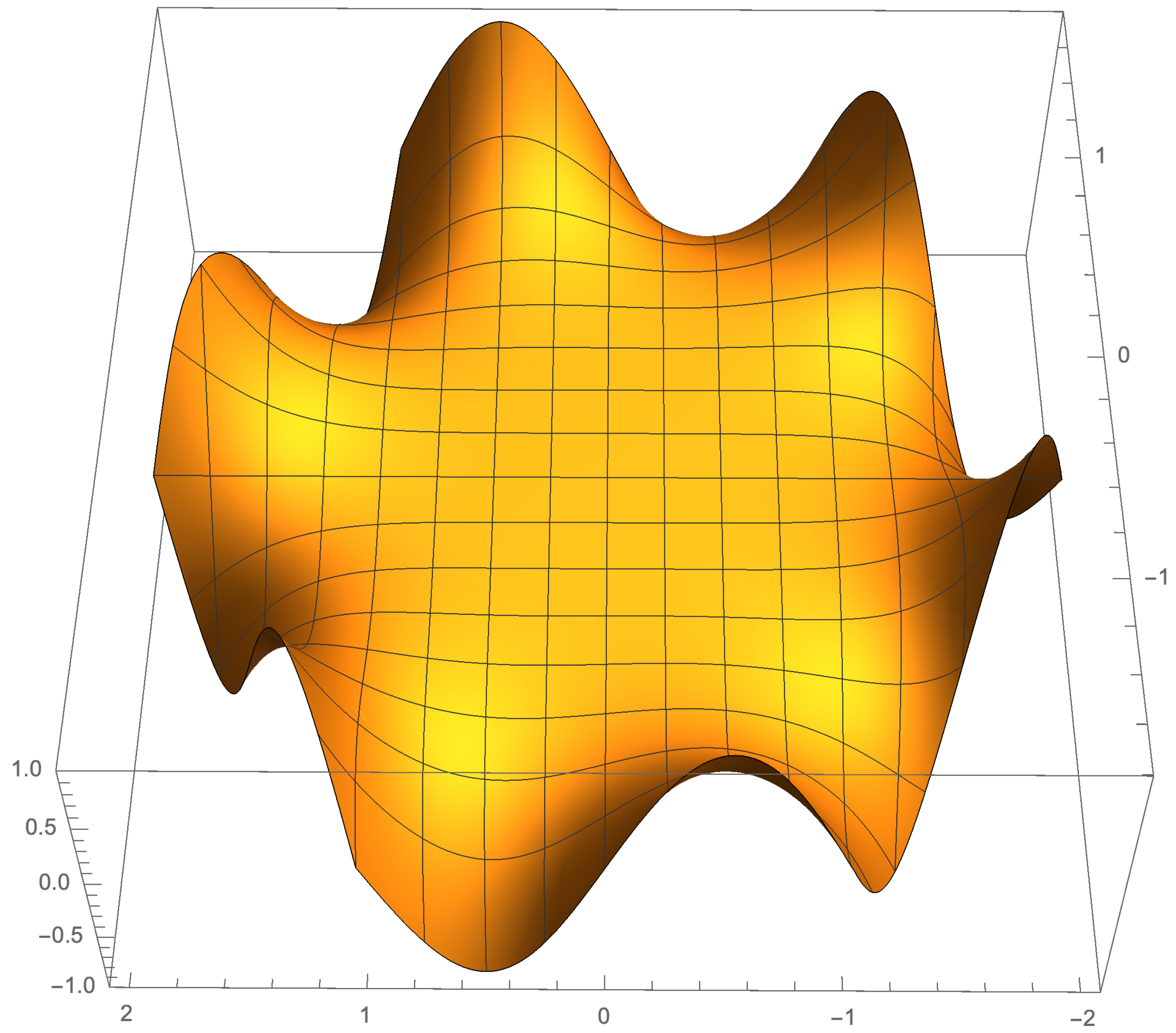
For the first example we employ the Dirichlet datum and the parameter ; see Figure 1.
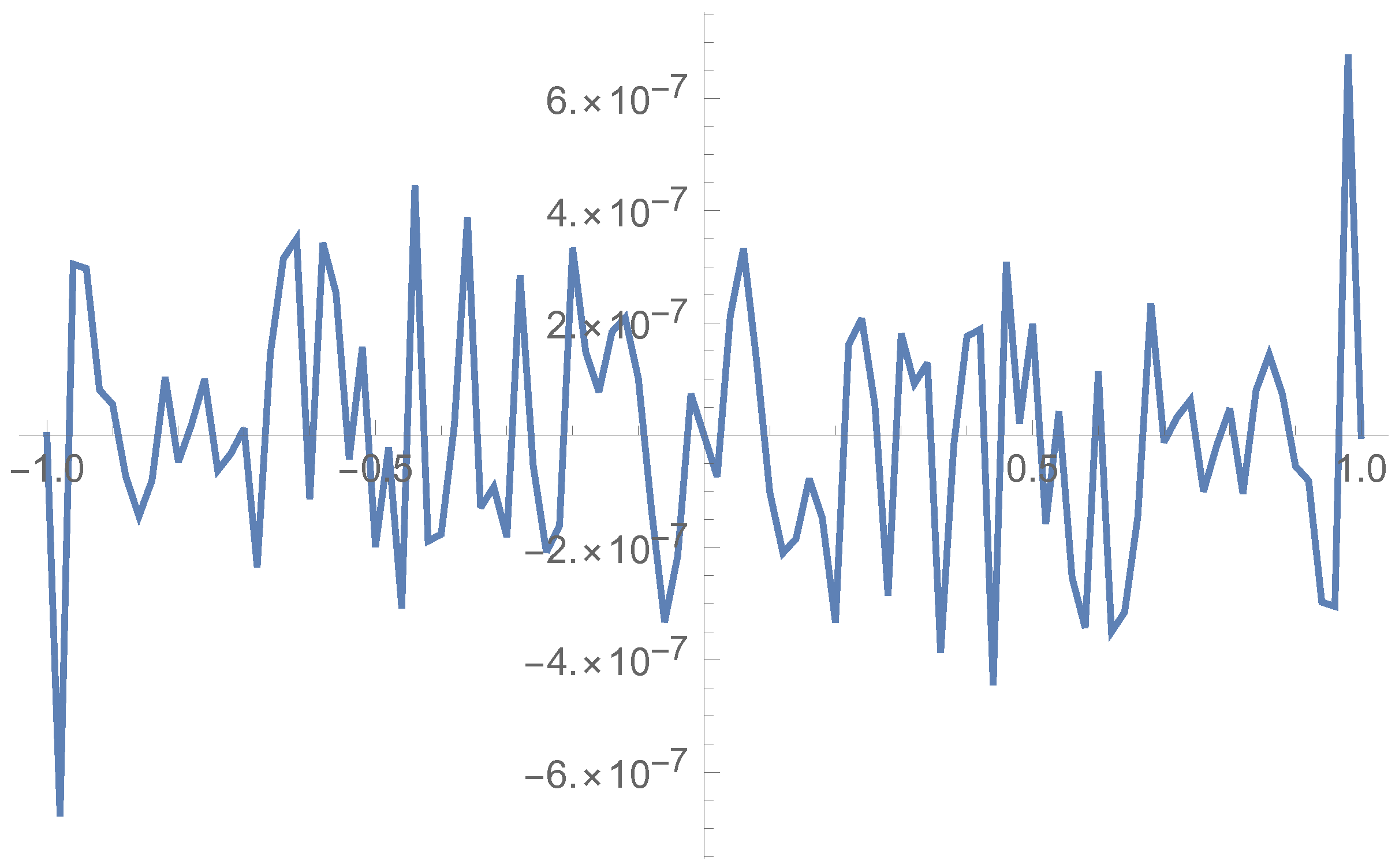
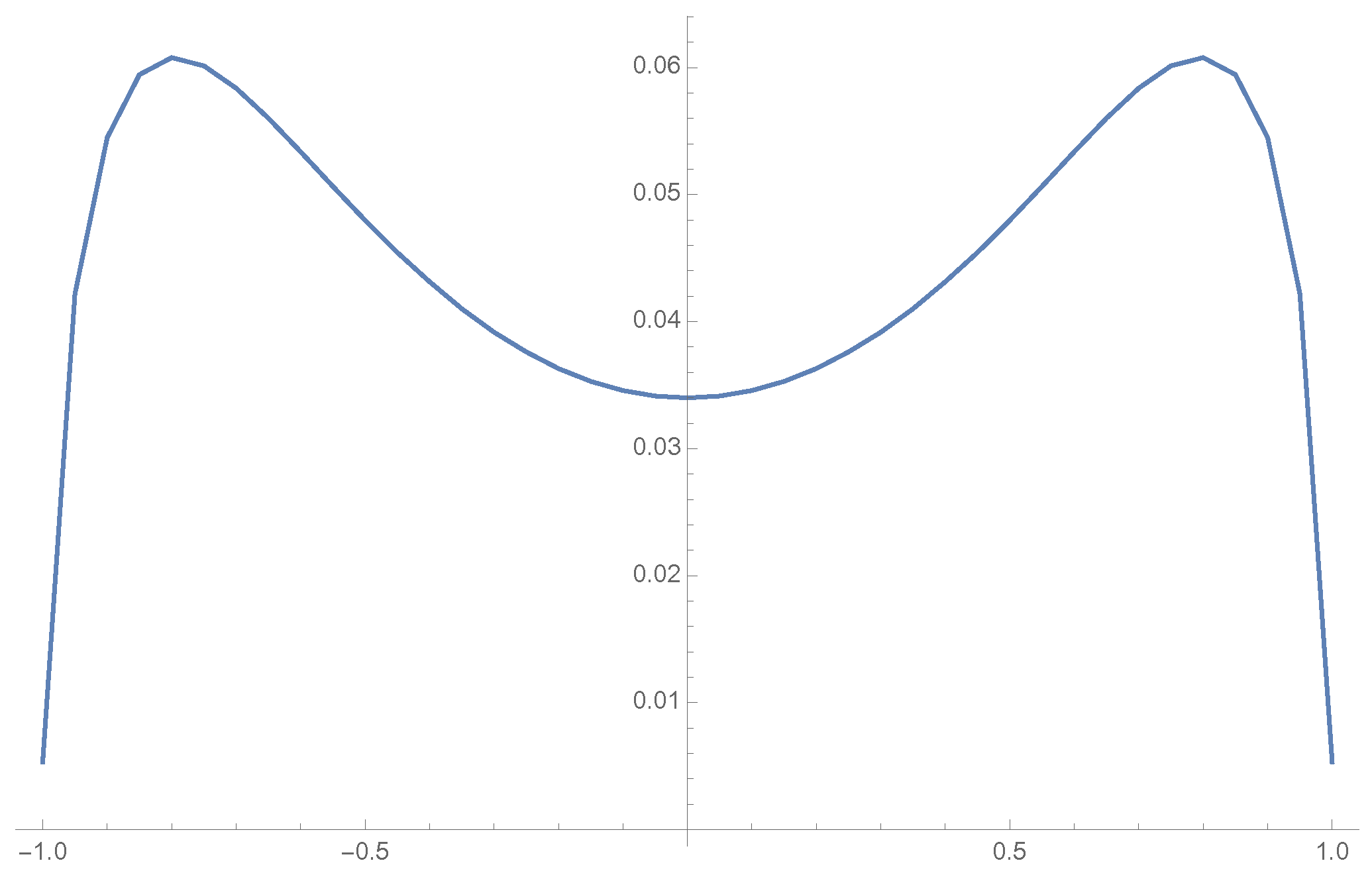
We also depict the deviation of from the function obtained by the integral representation (34) evaluated at the side of the hexagon, namely at and ; see Figure 2.
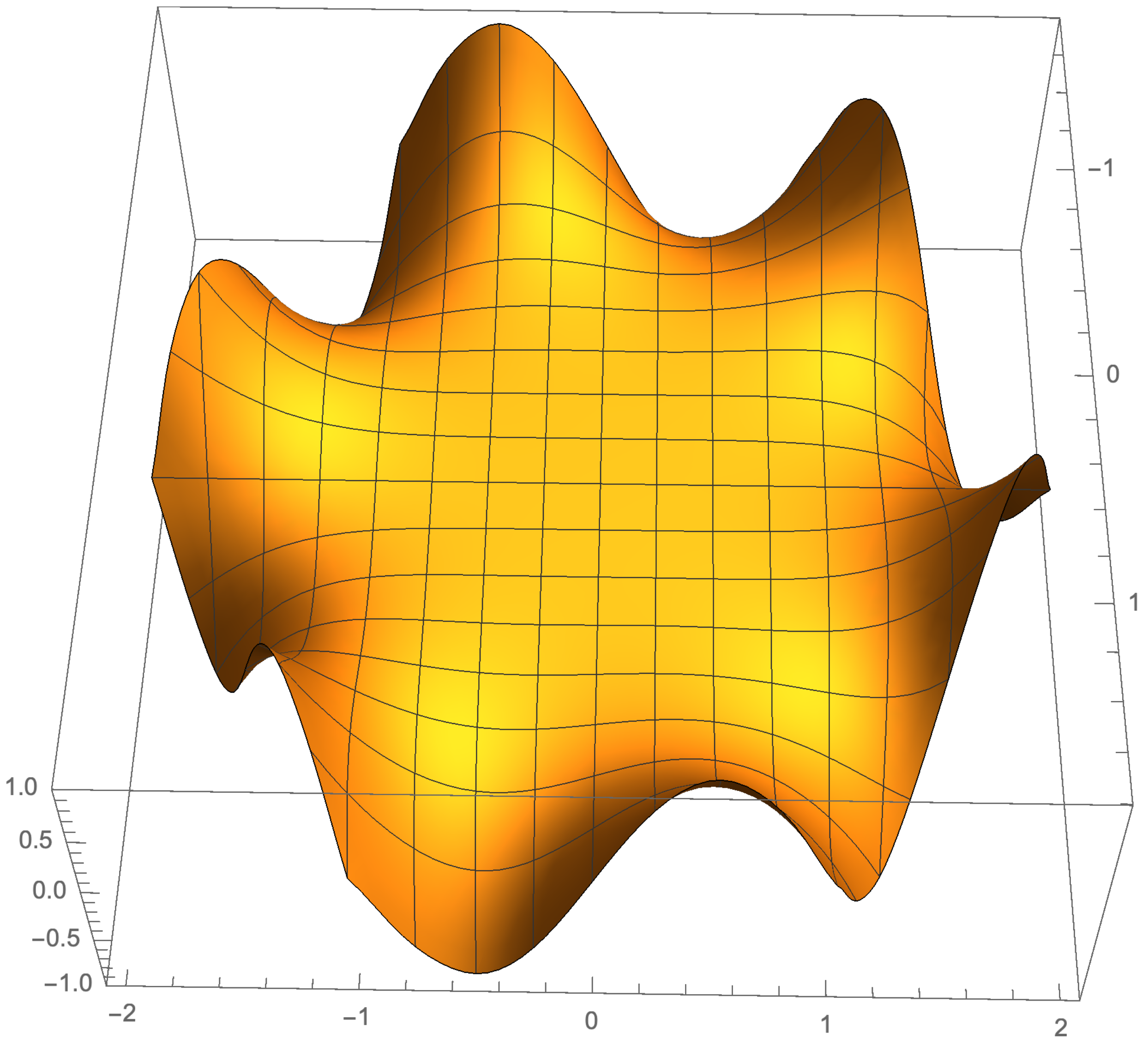
For the second example we employ the Dirichlet datum and the parameter ; see Figure 3.
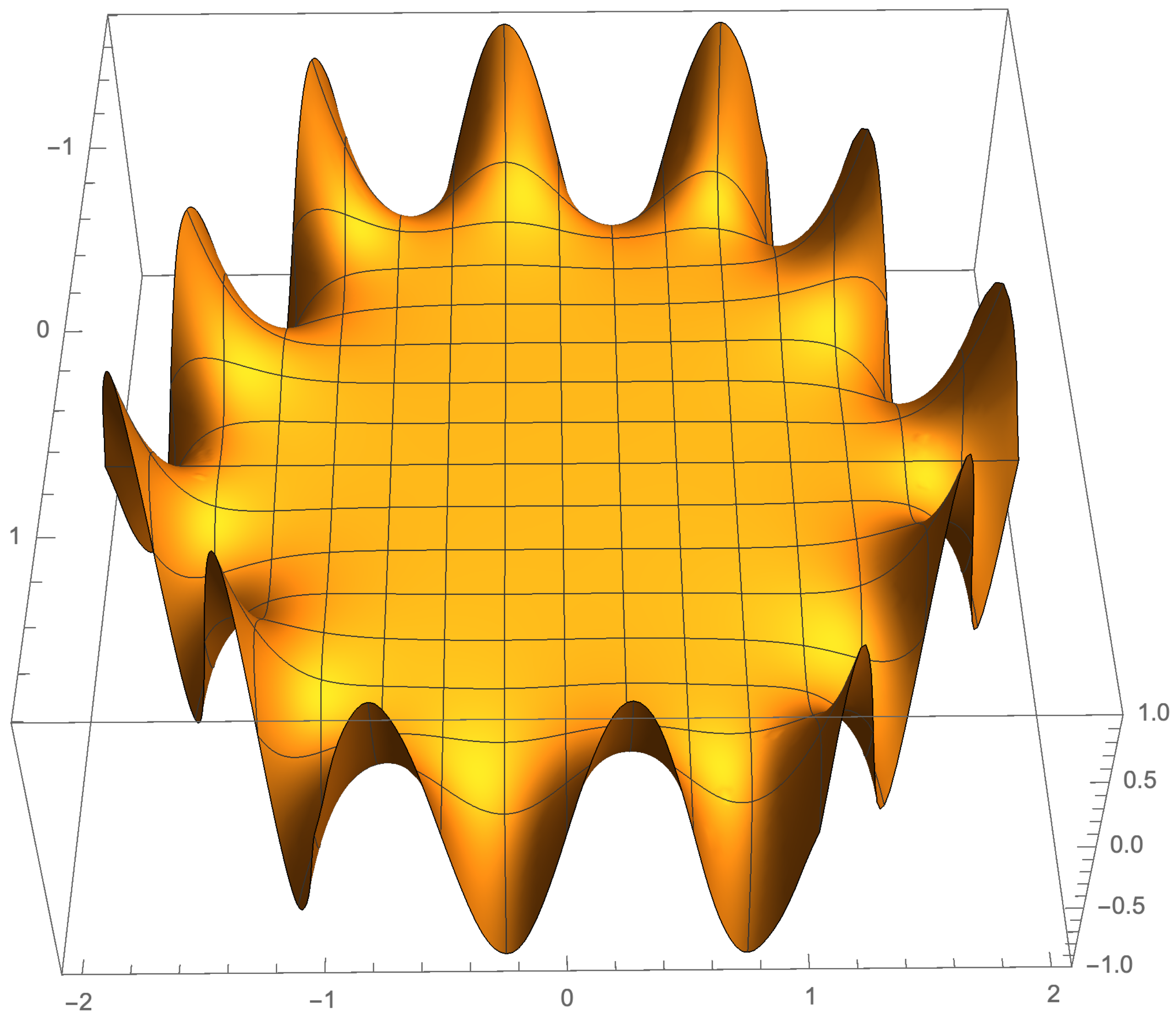
For the third example we employ the Dirichlet datum and the parameter ; see Figure 4.
5.2. Even Case
In this case we employ the Dirichlet datum and the parameter at the known part of the rhs of the formula (37), namely the expression
where and are given by (38) and (39), respectively; see Figure 5.
We also depict the deviation of from the above expression evaluated at the side of the hexagon, namely at and . This is equal to the contribution , with given by (40); see Figure 6.
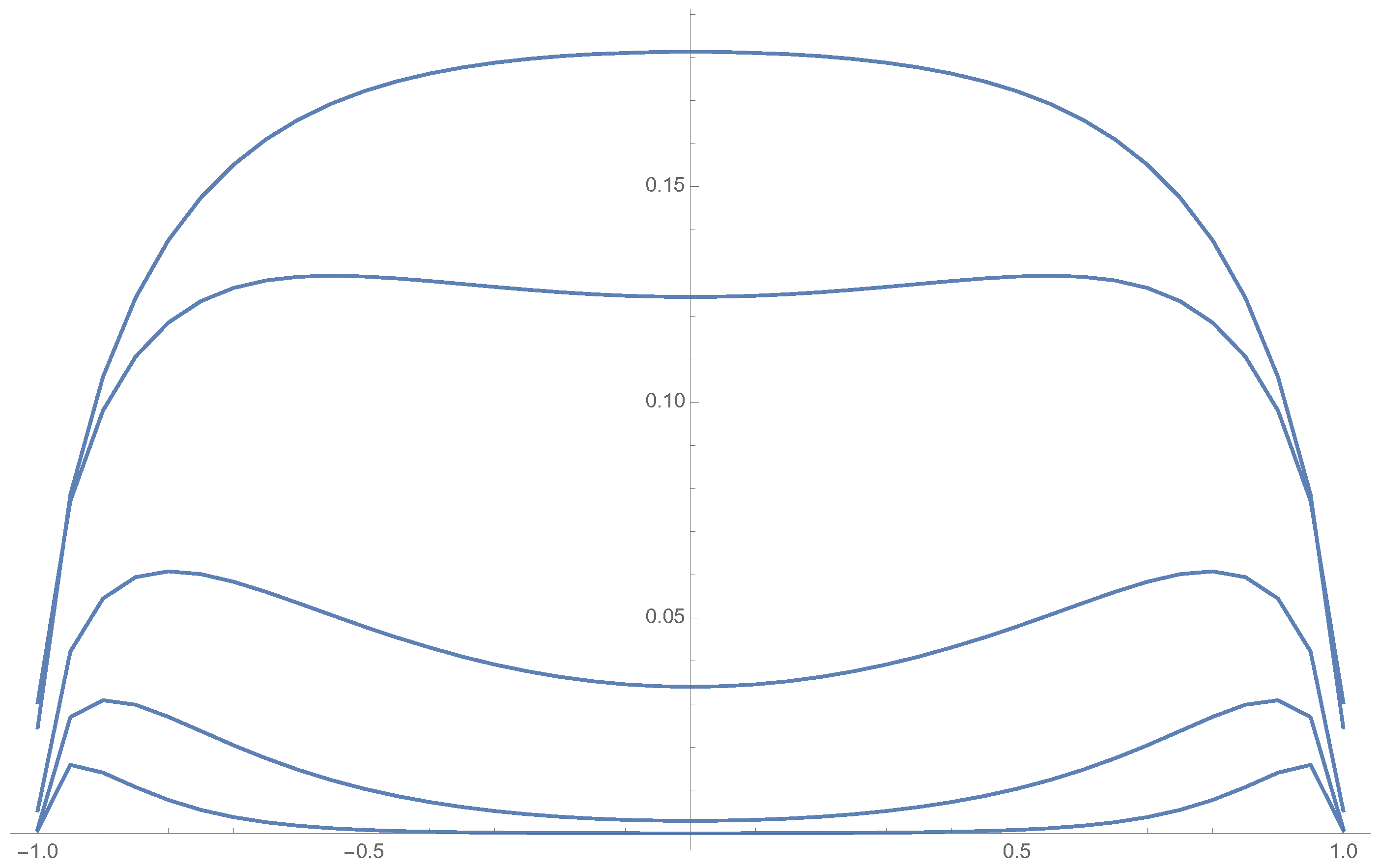
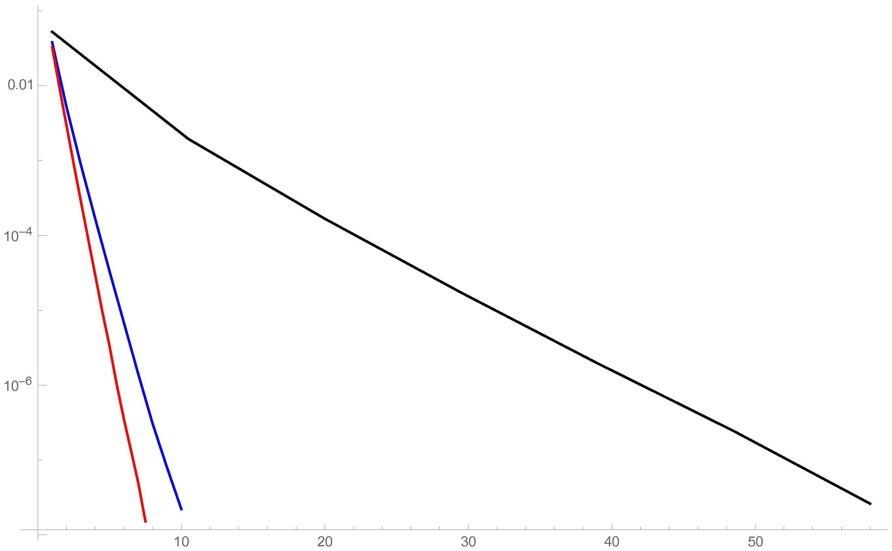
Furthermore, we depict the latter contribution for the different values of , where it is clearly shown that the error decreases drastically with the increase of ; see Figure 7. We observe exponential decay for : in Figure 8 we depict the deviation from the actual Dirichlet data for three points on side (1) of the hexagon, namely , with in the intervals , respectively.
6. Conclusions
In this work we have presented the explicit solution of a particular boundary value problem for the modified Helmholtz equation in a regular hexagon: we have solved the case where the same Dirichlet datum is prescribed in all sides of the hexagon, and this function is odd. This explicit solution is described in Proposition 1. We have also obtained an approximate analytical representation for the solution for the case that is even. The exact representation is given by Equation (37), where the terms and are given in terms of , but the terms involve the unknown Neumann boundary value. However, these terms are exponentially small as . Thus, for the case of large , Equation (37) provides the solution to this problem with an exponentially small error. The above analytical results were verified numerically in Section 5. The rigorous investigation on the analytical and numerical accuracy of the latter approximate formula will be presented in future work.
It should be noted that the arbitrary Dirichlet problem can be decomposed into 6 separate and simpler Dirichlet BVPs, which are defined in Section 2.3; the first of these BVPs is the symmetric Dirichlet problem. The analysis of the remaining problems is a work in progress.
Author Contributions
Conceptualization, K.K. and A.S.F.; methodology, K.K. and A.S.F.; validation, K.K. and A.S.F.; formal analysis, K.K. and A.S.F.; investigation, K.K. and A.S.F.; writing–original draft preparation, K.K. and A.S.F.; writing–review and editing, K.K. and A.S.F.; visualization, K.K. and A.S.F. All authors have read and agreed to the published version of the manuscript.
Funding
A.S.F. was supported by EPSRC, UK, via a senior fellowship.
Conflicts of Interest
The authors declare no conflict of interest.
References
- Fokas, A.S. A unified transform method for solving linear and certain nonlinear PDEs. Proc. R. Soc. Lond. A Math. Phys. Eng. Sci. 1997, 453, 1411–1443. [Google Scholar] [CrossRef]
- Fokas, A.S. On the integrability of linear and nonlinear partial differential equations. J. Math. Phys. 2000, 41, 4188–4237. [Google Scholar] [CrossRef]
- Fokas, A.S. A new transform method for evolution partial differential equations. IMA J. Appl. Math. 2002, 67, 559–590. [Google Scholar] [CrossRef]
- Biondini, G.; Wang, D. Initial-boundary-value problems for discrete linear evolution equations. IMA J. Appl. Math. 2010, 75, 968–997. [Google Scholar] [CrossRef]
- Deconinck, B.; Trogdon, T.; Vasan, V. The method of Fokas for solving linear partial differential equations. SIAM Rev. 2014, 56, 159–186. [Google Scholar] [CrossRef]
- Fokas, A.S. A Unified Approach to Boundary Value Problems; SIAM: Garden Grove, CA, USA, 2008. [Google Scholar]
- Pelloni, B. The spectral representation of two-point boundary-value problems for third-order linear evolution partial differential equations. Proc. R. Soc. Lond. A Math. Phys. Eng. Sci. 2005, 461, 2965–2984. [Google Scholar] [CrossRef]
- Pelloni, B.; Smith, D.A. Spectral theory of some non-selfadjoint linear differential operators. Proc. R. Soc. A Math. Phys. Eng. Sci. 2013, 469, 20130019. [Google Scholar] [CrossRef]
- Pelloni, B.; Smith, D.A. Evolution PDEs and augmented eigenfunctions. Half-line. J. Spectr. Theory 2016, 6, 185–213. [Google Scholar] [CrossRef] [Green Version]
- Smith, D.A. Well-posed two-point initial-boundary value problems with arbitrary boundary conditions. In Mathematical Proceedings of the Cambridge Philosophical Society; Cambridge University Press: Cambridge, UK, 2012; Volume 152, pp. 473–496. [Google Scholar]
- Fokas, A.S. Two-dimensional linear partial differential equations in a convex polygon. Proc. R. Soc. Lond. Ser. A Math. Phys. Eng. Sci. 2001, 457, 371–393. [Google Scholar] [CrossRef]
- Kalimeris, K. INITIAL and Boundary Value Problems in Two and Three Dimensions. Ph.D. Thesis, University of Cambridge, Cambridge, UK, 2010. [Google Scholar]
- Spence, E.A. Boundary Value Problems for Linear Elliptic PDEs. Ph.D. Thesis, University of Cambridge, Cambridge, UK, 2011. [Google Scholar]
- Batal, A.; Fokas, A.S.; Özsari, T. Uniform transform method for boundary value problems involving mixed derivatives. arXiv 2020, arXiv:2002.01057. [Google Scholar]
- Fokas, A.S.; Himonas, A.A.; Mantzavinos, D. The nonlinear Schrödinger equation on the half-line. Trans. Am. Math. Soc. 2017, 369, 681–709. [Google Scholar] [CrossRef] [Green Version]
- Himonas, A.A.; Mantzavinos, D. On the Initial-Boundary Value Problem for the Linearized Boussinesq Equation. Stud. Appl. Math. 2015, 134, 62–100. [Google Scholar] [CrossRef]
- Himonas, A.A.; Mantzavinos, D.; Yan, F. Initial-boundary value problems for a reaction-diffusion equation. J. Math. Phys. 2019, 60, 081509. [Google Scholar] [CrossRef]
- Özsari, T.; Yolcu, N. The initial-boundary value problem for the biharmonic Schrödinger equation on the half-line. Commun. Pure Appl. Anal. 2019, 18, 3285–3316. [Google Scholar] [CrossRef] [Green Version]
- Kalimeris, K.; Özsarı, T. An elementary proof of the lack of null controllability for the heat equation on the half line. Appl. Math. Lett. 2020, 104, 106241. [Google Scholar] [CrossRef] [Green Version]
- Crowdy, D.G.; Davis, A.M. Stokes flow singularities in a two-dimensional channel: A novel transform approach with application to microswimming. Proc. R. Soc. A 2013, 469, 20130198. [Google Scholar]
- Deconinck, B.; Oliveras, K. The instability of periodic surface gravity waves. J. Fluid Mech. 2011, 675, 141–167. [Google Scholar] [CrossRef] [Green Version]
- Fokas, A.S.; Kalimeris, K. Water waves with moving boundaries. J. Fluid Mech. 2017, 832, 641–665. [Google Scholar] [CrossRef]
- Oliveras, K. Stability of Periodic Surface Gravity Water Waves. Ph.D. Thesis, University of Washington, Seattle, WA, USA, 2009. [Google Scholar]
- Plümacher, D.; Oberlack, M.; Wang, Y.; Smuda, M. On a non-linear droplet oscillation theory via the unified method. Phys. Fluids 2020, 32, 067104. [Google Scholar] [CrossRef]
- Vasan, V.; Deconinck, B. The inverse water wave problem of bathymetry detection. J. Fluid Mech. 2013, 714, 562–590. [Google Scholar] [CrossRef] [Green Version]
- Ablowitz, M.J.; Fokas, A.S.; Musslimani, Z.H. On a new non-local formulation of water waves. J. Fluid Mech. 2006, 562, 313–343. [Google Scholar] [CrossRef] [Green Version]
- Nicholls, D. A high-order perturbation of surfaces (HOPS) approach to Fokas integral equations: Three-dimensional layered-media scattering. Q. Appl. Math. 2016, 74, 61–87. [Google Scholar] [CrossRef]
- Ashton, A.C.L. Laplace’s equation on convex polyhedra via the unified method. Proc. R. Soc. A Math. Phys. Eng. Sci. 2015, 471, 20140884. [Google Scholar] [CrossRef] [Green Version]
- Crowdy, D. A transform method for Laplace’s equation in multiply connected circular domains. IMA J. Appl. Math. 2015, 80, 1902–1931. [Google Scholar] [CrossRef] [Green Version]
- Dassios, G.; Fokas, A.S. The basic elliptic equations in an equilateral triangle. Proc. R. Soc. A Math. Phys. Eng. Sci. 2005, 461, 2721–2748. [Google Scholar] [CrossRef] [Green Version]
- Fokas, A.S.; Kapaev, A.A. A Riemann-Hilbert approach to the Laplace equation. J. Math. Anal. Appl. 2000, 251, 770–804. [Google Scholar] [CrossRef] [Green Version]
- Fokas, A.S.; Kapaev, A.A. On a transform method for the Laplace equation in a polygon. IMA J. Appl. Math. 2003, 68, 355–408. [Google Scholar] [CrossRef]
- Luca, E.; Crowdy, D.G. A transform method for the biharmonic equation in multiply connected circular domains. IMA J. Appl. Math. 2018, 83, 942–976. [Google Scholar] [CrossRef]
- Antipov, Y.A.; Fokas, A.S. The modified Helmholtz equation in a semi-strip. In Mathematical Proceedings of the Cambridge Philosophical Society; Cambridge University Press: Cambridge, UK, 2005; Volume 138, pp. 339–365. [Google Scholar]
- Ashton, A.C.L. On the rigorous foundations of the Fokas method for linear elliptic partial differential equations. Proc. R. Soc. A Math. Phys. Eng. Sci. 2012, 468, 1325–1331. [Google Scholar] [CrossRef]
- Ashton, A.C.L. The Spectral Dirichlet–Neumann Map for Laplace’s Equation in a Convex Polygon. SIAM J. Math. Anal. 2013, 45, 3575–3591. [Google Scholar] [CrossRef] [Green Version]
- Colbrook, M.J. Extending the unified transform: Curvilinear polygons and variable coefficient PDEs. IMA J. Numer. Anal. 2020, 40, 976–1004. [Google Scholar] [CrossRef]
- Colbrook, M.J.; Flyer, N.; Fornberg, B. On the Fokas method for the solution of elliptic problems in both convex and non-convex polygonal domains. J. Comput. Phys. 2018, 374, 996–1016. [Google Scholar] [CrossRef] [Green Version]
- Colbrook, M.J.; Fokas, A.S. Computing eigenvalues and eigenfunctions of the Laplacian for convex polygons. Appl. Numer. Math. 2018, 126, 1–17. [Google Scholar] [CrossRef]
- Colbrook, M.J.; Fokas, A.S.; Hashemzadeh, P. A Hybrid Analytical-Numerical Technique for Elliptic PDEs. SIAM J. Sci. Comput. 2019, 41, A1066–A1090. [Google Scholar] [CrossRef]
- de Barros, F.P.J.; Colbrook, M.J.; Fokas, A.S. A hybrid analytical-numerical method for solving advection-dispersion problems on a half-line. Int. J. Heat Mass Transf. 2019, 139, 482–491. [Google Scholar] [CrossRef]
- Davis, C.I.R.; Fornberg, B. A spectrally accurate numerical implementation of the Fokas transform method for Helmholtz-type PDEs. Complex Var. Elliptic Equ. 2014, 59, 564–577. [Google Scholar] [CrossRef]
- Fokas, A.S.; Nachbin, A. Water waves over a variable bottom: A non-local formulation and conformal mappings. J. Fluid Mech. 2012, 695, 288–309. [Google Scholar] [CrossRef]
- Fornberg, B.; Flyer, N. A numerical implementation of Fokas boundary integral approach: Laplace’s equation on a polygonal domain. Proc. R. Soc. A Math. Phys. Eng. Sci. 2011, 467, 2983–3003. [Google Scholar] [CrossRef] [Green Version]
- Grylonakis, E.N.G.; Filelis-Papadopoulos, C.K.; Gravvanis, G.A. A class of unified transform techniques for solving linear elliptic PDEs in convex polygons. Appl. Numer. Math. 2018, 129, 159–180. [Google Scholar] [CrossRef]
- Hashemzadeh, P.; Fokas, A.S.; Smitheman, S.A. A numerical technique for linear elliptic partial differential equations in polygonal domains. Proc. Math. Phys. Eng. Sci. 2015, 471, 20140747. [Google Scholar] [CrossRef]
- Trogdon, T.; Biondini, G. Evolution partial differential equations with discontinuous data. Q. Appl. Math. 2019, 77, 689–726. [Google Scholar] [CrossRef]
- Lamé, G. Mémoire sur la propagation de la chaleur dans les polyèdres, et principalement dans le prisme triangulaire régulier. J. I’Ecole Poly Tech. 1833, 22, 194–251. [Google Scholar]
- Fokas, A.S.; Kalimeris, K. Eigenvalues for the Laplace operator in the interior of an equilateral triangle. Comput. Methods Funct. Theory 2014, 14, 1–33. [Google Scholar] [CrossRef]
- Pinsky, M.A. The eigenvalues of an equilateral triangle. SIAM J. Math. Anal. 1980, 11, 819–827. [Google Scholar] [CrossRef]
- Pinsky, M.A. Completeness of the eigenfunctions of the equilateral triangle. SIAM J. Math. Anal. 1985, 16, 848–851. [Google Scholar] [CrossRef]
- Práger, M. Eigenvalues and eigenfunctions of the Laplace operator on an equilateral triangle. Appl. Math. 1998, 43, 311–320. [Google Scholar] [CrossRef] [Green Version]
- Terras, R.; Swanson, R. Image methods for constructing Green’s functions and eigenfunctions for domains with plane boundaries. J. Math. Phys. 1980, 21, 2140–2153. [Google Scholar] [CrossRef]
- McCartin, B.J. Eigenstructure of the equilateral triangle, Part I: The Dirichlet problem. Siam Rev. 2003, 45, 267–287. [Google Scholar] [CrossRef]
- McCartin, B.J. Eigenstructure of the equilateral triangle, Part II: The Neumann problem. Math. Probl. Eng. 2002, 8. [Google Scholar] [CrossRef]
- McCartin, B.J. Laplacian Eigenstructure of the Equilateral Triangle; Hikari Limited: Rousse, Bulgaria, 2011. [Google Scholar]
Figure 1.
The solution q given by (34) for and .
Figure 1.
The solution q given by (34) for and .

Figure 2.
The deviation of q (given by (34)) from the actual Dirichlet datum evaluated at the side of the hexagon; here we employ , and .
Figure 2.
The deviation of q (given by (34)) from the actual Dirichlet datum evaluated at the side of the hexagon; here we employ , and .

Figure 3.
The solution q given by (34) for and .
Figure 3.
The solution q given by (34) for and .

Figure 4.
The solution q given by (34) for and .
Figure 4.
The solution q given by (34) for and .

Figure 5.
The known part of the solution q given by (41) for and .
Figure 5.
The known part of the solution q given by (41) for and .

Figure 6.
The deviation of the known part of the solution q given by (41) from the actual Dirichlet datum , and , evaluated at the side of the hexagon.
Figure 6.
The deviation of the known part of the solution q given by (41) from the actual Dirichlet datum , and , evaluated at the side of the hexagon.

Figure 7.
The deviation of the known part of the solution q given by (41) from the actual Dirichlet datum and , evaluated at the side of the hexagon. This deviation is depicted for the different values of , and it decreases drastically with the increase of .
Figure 7.
The deviation of the known part of the solution q given by (41) from the actual Dirichlet datum and , evaluated at the side of the hexagon. This deviation is depicted for the different values of , and it decreases drastically with the increase of .

Figure 8.
The deviation of the known part of the solution q given by (41) from the actual Dirichlet datum , evaluated at three points of side (1) of the hexagon, namely in red, in blue, in black. The deviation is depicted against and it displays exponential decay.
Figure 8.
The deviation of the known part of the solution q given by (41) from the actual Dirichlet datum , evaluated at three points of side (1) of the hexagon, namely in red, in blue, in black. The deviation is depicted against and it displays exponential decay.

© 2020 by the authors. Licensee MDPI, Basel, Switzerland. This article is an open access article distributed under the terms and conditions of the Creative Commons Attribution (CC BY) license (http://creativecommons.org/licenses/by/4.0/).
Share and Cite
MDPI and ACS Style
Kalimeris, K.; Fokas, A.S. The Modified Helmholtz Equation on a Regular Hexagon—The Symmetric Dirichlet Problem. Axioms 2020, 9, 89. https://doi.org/10.3390/axioms9030089
AMA Style
Kalimeris K, Fokas AS. The Modified Helmholtz Equation on a Regular Hexagon—The Symmetric Dirichlet Problem. Axioms. 2020; 9(3):89. https://doi.org/10.3390/axioms9030089
Chicago/Turabian StyleKalimeris, Konstantinos, and Athanassios S. Fokas. 2020. "The Modified Helmholtz Equation on a Regular Hexagon—The Symmetric Dirichlet Problem" Axioms 9, no. 3: 89. https://doi.org/10.3390/axioms9030089
Note that from the first issue of 2016, this journal uses article numbers instead of page numbers. See further details here.