Initial Value Problem For Nonlinear Fractional Differential Equations With ψ-Caputo Derivative Via Monotone Iterative Technique


Abstract
:
1. Introduction
2. Preliminaries
3. Main Results
- (H1)
- (H2)
- There exists a constant such that
- Step 1: We show that the sequences are lower and upper solutions of problem (1), respectively and the following relation holds
- Step 2: The sequences , converge uniformly to their limit functions , respectively.
- Step 3: We prove that and are extremal solutions of problem (1) in .
- (H3)
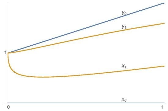
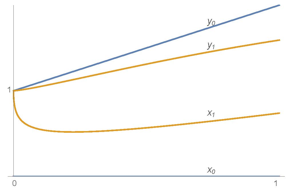
4. An Example
5. Conclusions
Author Contributions
Funding
Conflicts of Interest
References
- Hilfer, R. Applications of Fractional Calculus in Physics; World Scientific: Singapore, 2000. [Google Scholar]
- Oldham, K.B. Fractional differential equations in electrochemistry. Adv. Eng. Softw. 2010, 41, 9–12. [Google Scholar] [CrossRef]
- Sabatier, J.; Agrawal, O.P.; Machado, J.A.T. Advances in Fractional Calculus-Theoretical Developments and Applications in Physics and Engineering; Springer: Dordrecht, The Netherlands, 2007. [Google Scholar]
- Tarasov, V.E. Fractional Dynamics: Application of Fractional Calculus to Dynamics of Particles, Fields and Media; Springer Science & Business Media: Berlin/Heidelberg, Germany, 2010. [Google Scholar]
- Abbas, S.; Benchohra, M.; N’Guŕékata, G.M. Topics in Fractional Differential Equations; Springer: New York, NY, USA, 2015. [Google Scholar]
- Abbas, S.; Benchohra, M.; Graef, J.R.; Henderson, J. Implicit Fractional Differential and Integral Equations: Existence and Stability; De Gruyter: Berlin, Germany, 2018. [Google Scholar]
- Abbas, S.; Benchohra, M.; N’Guŕékata, G.M. Advanced Fractional Differential and Integral Equations; Nova Sci. Publ.: New York, NY, USA, 2014. [Google Scholar]
- Kilbas, A.A.; Srivastava, H.M.; Trujillo, J.J. Theory and Applications of Fractional Differential Equations; vol. 204 of North-Holland Mathematics Sudies; Elsevier Science B.V.: Amsterdam, The Netherlands, 2006. [Google Scholar]
- Miller, K.S.; Ross, B. An Introduction to Fractional Calculus and Fractional Differential Equations; Wiley: New York, NY, USA, 1993. [Google Scholar]
- Podlubny, I. Fractional Differential Equations; Academic Press: San Diego, CA, USA, 1999. [Google Scholar]
- Zhou, Y. Basic Theory of Fractional Differential Equations; World Scientific: Singapore, 2014. [Google Scholar]
- Zhou, Y. Fractional Evolution Equations and Inclusions; Analysis and Control; Elsevier, Acad. Press: Cambridge, MA, USA, 2016. [Google Scholar]
- Agarwal, R.P.; Benchohra, M.; Hamani, S. A survey onexistence results for boundary value problems of nonlinear fractional differential equations and inclusions. Acta Appl. Math. 2010, 109, 973–1033. [Google Scholar] [CrossRef]
- Benchohra, M.; Graef, J.R.; Hamani, S. Existence results for boundary value problems with non-linear fractional differential equations. Appl. Anal. 2008, 87, 851–863. [Google Scholar] [CrossRef]
- Benchohra, M.; Hamani, S.; Ntouyas, S.K. Boundary value problems for differential equations with fractional order and nonlocal conditions. Nonlinear Anal. 2009, 71, 2391–2396. [Google Scholar] [CrossRef]
- Benchohra, M.; Lazreg, J.E. Existence results for nonlinear implicit fractional differential equations. Surv. Math. Appl. 2014, 9, 79–92. [Google Scholar]
- Almeida, R. A Caputo fractional derivative of a function with respect to another function. Commun. Nonlinear Sci. 2017, 44, 460–481. [Google Scholar] [CrossRef]
- Abdo, M.S.; Panchal, S.K.; Saeed, A.M. Fractional boundary value problem with ψ-Caputo fractional derivative. Proc. Math. Sci. 2019, 129, 14. [Google Scholar] [CrossRef]
- Almeida, R. Fractional Differential Equations with Mixed Boundary Conditions. Bull. Malays. Math. Sci. Soc. 2019, 42, 1687–1697. [Google Scholar] [CrossRef] [Green Version]
- Almeida, R.; Malinowska, A.B.; Monteiro, M.T.T. Fractional differential equations with a Caputo derivative with respect to a kernel function and their applications. Math. Meth. Appl. Sci. 2018, 41, 336–352. [Google Scholar] [CrossRef] [Green Version]
- Almeida, R.; Malinowska, A.B.; Odzijewicz, T. Optimal Leader-Follower Control for the Fractional Opinion Formation Model. J. Optim. Theory Appl. 2019, 182, 1171–1185. [Google Scholar] [CrossRef] [Green Version]
- Almeida, R.; Jleli, M.; Samet, B. A numerical study of fractional relaxation-oscillation equations involving ψ-Caputo fractional derivative. Rev. R. Acad. Cienc. Exactas Fís. Nat. Ser. A Mat. RACSAM 2019, 113, 1873–1891. [Google Scholar] [CrossRef]
- Samet, B.; Aydi, H. Lyapunov-type inequalities for an anti-periodic fractional boundary value problem involving ψ-Caputo fractional derivative. J. Inequal. Appl. 2018, 2018, 286. [Google Scholar] [CrossRef] [PubMed] [Green Version]
- Abbas, S.; Benchohra, M.; Samet, B.; Zhou, Y. Coupled implicit Caputo fractional q-difference systems. Adv. Diff. Equ. 2019, 2019, 527. [Google Scholar] [CrossRef]
- Abbas, S.; Benchohra, M.; Hamidi, N.; Henderson, J. Caputo–Hadamard fractional differential equations in Banach spaces. Fract. Calc. Appl. Anal. 2018, 21, 1027–1045. [Google Scholar] [CrossRef]
- Abbas, S.; Benchohra, M.; Hamani, S.; Henderson, J. Upper and lower solutions method for Caputo-Hadamard fractional differential inclusions. Math. Morav. 2019, 23, 107–118. [Google Scholar] [CrossRef]
- Aghajani, A.; Pourhadi, E.; Trujillo, J.J. Application of measure of noncompactness to a Cauchy problem for fractional differential equations in Banach spaces. Fract. Calc. Appl. Anal. 2013, 16, 962–977. [Google Scholar] [CrossRef]
- Kucche, K.D.; Mali, A.D.; Sousa, J.V.C. On the nonlinear Ψ-Hilfer fractional differential equations. Comput. Appl. Math. 2019, 38, 25. [Google Scholar] [CrossRef]
- Wu, G.C.; Zeng, D.Q.; Baleanu, D. Fractional impulsive differential equations: Exact solutions, integral equations and short memory case. Fract. Calc Appl. Anal. 2019, 22, 180–192. [Google Scholar] [CrossRef]
- Wu, G.C.; Deng, Z.G.; Baleanu, D.; Zeng, D.Q. New variable order fractional chaotic systems for fast image encryption. Chaos 2019, 29, 11. [Google Scholar] [CrossRef]
- Ali, S.; Shah, K.; Jarad, F. On stable iterative solutions for a class of boundary value problem of nonlinear fractional order differential equations. Math. Methods Appl. Sci. 2019, 42, 969–981. [Google Scholar] [CrossRef]
- Al-Refai, M.; Ali Hajji, M. Monotone iterative sequences for nonlinear boundary value problems of fractional order. Nonlinear Anal. 2011, 74, 3531–3539. [Google Scholar] [CrossRef]
- Chen, C.; Bohner, M.; Jia, B. Method of upper and lower solutions for nonlinear Caputo fractional difference equations and its applications. Fract. Calc. Appl. Anal. 2019, 22, 1307–1320. [Google Scholar] [CrossRef]
- Dhaigude, D.; Rizqan, B. Existence and uniqueness of solutions of fractional differential equations with deviating arguments under integral boundary conditions. Kyungpook Math. J. 2019, 59, 191–202. [Google Scholar]
- Fazli, H.; Sun, H.; Aghchi, S. Existence of extremal solutions of fractional Langevin equation involving nonlinear boundary conditions. Int. J. Comput. Math. 2020. [Google Scholar] [CrossRef]
- Lin, X.; Zhao, Z. Iterative technique for a third-order differential equation with three-point nonlinear boundary value conditions. Electron. J. Qual. Theory Differ. Equ. 2016, 12, 10. [Google Scholar] [CrossRef]
- Ma, K.; Han, Z.; Sun, S. Existence and uniqueness of solutions for fractional q-difference Schrödinger equations. J. Appl. Math. Comput. 2020, 62, 611–620. [Google Scholar] [CrossRef]
- Mao, J.; Zhao, Z.; Wang, C. The unique iterative positive solution of fractional boundary value problem with q-difference. Appl. Math. Lett. 2020, 100, 106002. [Google Scholar] [CrossRef]
- Meng, S.; Cui, Y. The extremal solution to conformable fractional differential equations involving integral boundary condition. Mathematics 2019, 7, 186. [Google Scholar] [CrossRef] [Green Version]
- Wang, G.; Sudsutad, W.; Zhang, L.; Tariboon, J. Monotone iterative technique for a nonlinear fractional q-difference equation of Caputo type. Adv. Diff. Equ. 2016, 2016, 211. [Google Scholar] [CrossRef] [Green Version]
- Yang, W. Monotone iterative technique for a coupled system of nonlinear Hadamard fractional differential equations. J. Appl. Math. Comput. 2019, 59, 585–596. [Google Scholar] [CrossRef]
- Zhang, S. Monotone iterative method for initial value problem involving Riemann-Liouville fractional derivatives. Nonlinear Anal. 2009, 71, 2087–2093. [Google Scholar] [CrossRef]
- Gorenflo, R.; Kilbas, A.A.; Mainardi, F.; Rogosin, S.V. Mittag–Leffler Functions, Related Topics and Applications; Springer: New York, NY, USA, 2014. [Google Scholar]
- Diethelm, K.; Ford, N.J. Analysis of fractional differential equations. J. Math. Anal. Appl. 2002, 265, 229–248. [Google Scholar] [CrossRef] [Green Version]
- Nieto, J.J. Maximum principles for fractional differential equations derived from Mittag-Leffler functions. Appl. Math. Lett. 2010, 23, 1248–1251. [Google Scholar] [CrossRef] [Green Version]
- Royden, H.L. Real Analysis, 3rd ed.; Macmillan Publishing Company: New York, NY, USA, 1988. [Google Scholar]

© 2020 by the authors. Licensee MDPI, Basel, Switzerland. This article is an open access article distributed under the terms and conditions of the Creative Commons Attribution (CC BY) license (http://creativecommons.org/licenses/by/4.0/).
Share and Cite
Derbazi, C.; Baitiche, Z.; Benchohra, M.; Cabada, A. Initial Value Problem For Nonlinear Fractional Differential Equations With ψ-Caputo Derivative Via Monotone Iterative Technique. Axioms 2020, 9, 57. https://doi.org/10.3390/axioms9020057
Derbazi C, Baitiche Z, Benchohra M, Cabada A. Initial Value Problem For Nonlinear Fractional Differential Equations With ψ-Caputo Derivative Via Monotone Iterative Technique. Axioms. 2020; 9(2):57. https://doi.org/10.3390/axioms9020057
Chicago/Turabian StyleDerbazi, Choukri, Zidane Baitiche, Mouffak Benchohra, and Alberto Cabada. 2020. "Initial Value Problem For Nonlinear Fractional Differential Equations With ψ-Caputo Derivative Via Monotone Iterative Technique" Axioms 9, no. 2: 57. https://doi.org/10.3390/axioms9020057