Article

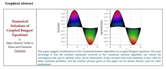
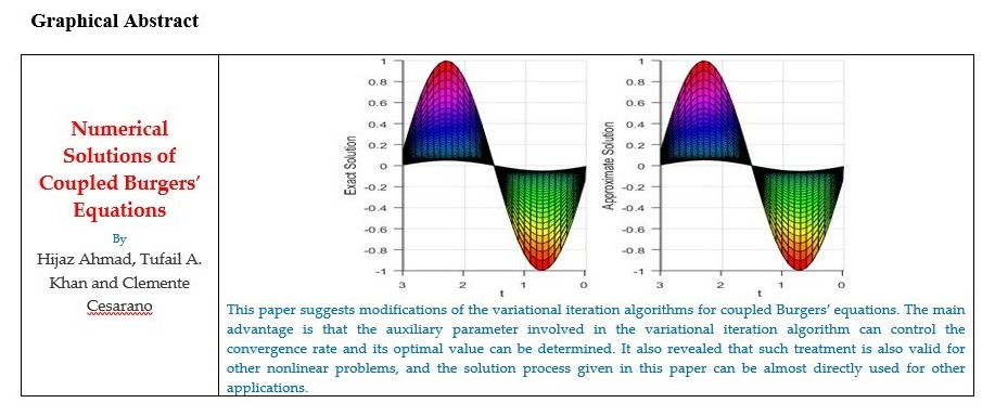
Numerical Solutions of Coupled Burgers’ Equations

1
Department of Basic Sciences, University of Engineering and Technology, Peshawar 25000, Pakistan
2
Section of Mathematics, International Telematic University Uninettuno, 39, 00186 Roma, Italy
*
Author to whom correspondence should be addressed.
Axioms 2019, 8(4), 119; https://doi.org/10.3390/axioms8040119
Submission received: 9 October 2019 / Revised: 20 October 2019 / Accepted: 21 October 2019 / Published: 23 October 2019

Abstract

:
In this article, two new modified variational iteration algorithms are investigated for the numerical solution of coupled Burgers’ equations. These modifications are made with the help of auxiliary parameters to speed up the convergence rate of the series solutions. Three numerical test problems are given to judge the behavior of the modified algorithms, and error norms are used to evaluate the accuracy of the method. Numerical simulations are carried out for different values of parameters. The results are also compared with the existing methods in the literature.

Graphical Abstract

1. Introduction

In recent years, coupled partial differential equations have been employed in various fields of engineering and applied sciences. Coupled Burgers’ equations are coupled partial differential equations (PDEs), and describe the approximation theory of flow through a shock wave traveling in a viscous fluid.
In this paper, the following type of coupled Burger equations will be investigated:
{ u t α 1 2 u x 2 + β 1 , 1 u x + β 1 , 2 u v x = 0 ,     t ( 0 ,   T ] ,         x [ a ,   b ] , v t α 2 2 v x 2 + β 2 , 2 v x + β 2 , 1 u v x = 0 ,     t ( 0 ,   T ] ,         x [ a ,   b ] ,
where α 1 and α 2 are positive and non-zero viscosity parameters, β 1 , 1 ,     β 1 , 2 ,     β 2 , 2 and β 2 , 1 are constants depend on the Stokes velocity. The initial and boundary conditions for coupled Burgers’ Equation (1) are the following:
{ u ( x , 0 ) = 1 ( x ) ,     x [ a ,   b ] , v ( x , 0 ) = 2 ( x ) ,     x [ a ,   b ] ,
{ u ( a , t ) = 1 ( t ) ,                 u ( b , t ) = 2 ( t )     x [ a ,   b ] , v ( a , t ) = 3 ( t ) ,                 v ( b , t ) = 4 ( t )     x [ a ,   b ] ,
Many authors have solved different types of coupled Burgers′ equations by different techniques such as the Fourier pseudospectral method [1] applied by Rashid and Ismail for one-dimensional coupled Burgers equations. A mesh-free interpolation method was employed by Islam et al. [2], where the radial basis function (RBF) collocation method has been formulated for the numerical treatment of coupled Burger equations and other nonlinear PDEs. Khater et al. [3] used the Chebyshev spectral collocation method, which has been developed using Chebyshev polynomials, and the Runge-Kutta 4th order method (RK4) method. Kya [4] used the decomposition method for the solution of a viscous coupled Burger equation, and obtained solutions in the form of a convergent power series. Mittal and Arora [5] proposed a scheme known as the Lai cubic B-spline collocation scheme for the solution of coupled viscous Burger equations, where the authors used a crank Nicholson scheme and cubic B-spline functions for time integration and space integration, respectively. Lai and Ma [6] proposed a new lattice Boltzmann model for the solution of coupled Burger equations, after selecting the distribution functions, Chapman–Enskog expansion was employed for the solution of coupled Burger equations. The Chebyshev–Legendre pseudospectral method [7] has been utilized by Rashid et al. for coupled viscous Burgers′ (VB) equations, where the leapfrog scheme and Chebyshev–Legendre Pseudo-Spectral method (CLPS) method were used for the time direction and space direction, respectively. Kumar and Pandit [8] used a composite numerical scheme for the numerical evaluation of coupled Burger equations, where the scheme was developed based on Haar wavelets and finite difference. Mohammadi and Mokhtari [9] used a reproducing Kernal method for an analytical solution in the form series of systems of Burger equations. At last, in 2019, Bak et al. [10] developed a new approach named a semi-Lagrangian approach for the numerical solution of coupled Burger equations. We compare our results with those of [10], and show the applicability of our proposed method to handle such problems as those that arise in applied science and engineering.
This paper aims to solve three types of coupled Burgers′ equations by employing variational iteration algorithm-II and one of the examples to be solved by modified variational iteration algorithm-I. The organization of the rest of the paper is as follows; in Section 2, we elucidate the variational iteration algorithm-II, in the next Section 3, the semi-numerical method is applied to three test problems, and a comparison is made with some other methods; lastly, some conclusions are drawn in the last Section 4.

2. Modified Variational Iteration Algorithm-II

Consider the nonlinear diffusion equation:
L [ w ( x , t ) ] + N [ w ( x , t ) ] = c ( x , t ) ,
where the terms   L [ w ( x , t ) ]   and N [ w ( x , t ) ] are linear and nonlinear terms in that order, while c ( x , t ) is the source term. For a given w 0 ( x , t ) , the approximate solution w n + 1 ( x , t ) of Equation (4) can be obtained as below:
w n + 1 ( x , t ) = w n ( x , t ) + 0 t λ ( s ) [ L { w n ( x , s ) } + N { w n ( x , s ) } ˜ c ( x , s ) ] d s ,    
In Equation (5), λ is a parameter, which is known as the Lagrange multiplier [11]. This Lagrange multiplier is obtained by variational theory, where w n ˜  is a term being restricted, which in turn gives δ w n ˜ = 0 and gives the following Lagrange multipliers:
λ = 1   f o r   m = 1 ,                                             λ = s t     f o r   m = 2 ,
and in general, the Lagrange multiplier for m ≥ 1:
λ = ( 1 ) m ( s t ) m 1 ( m 1 ) ! .
Putting the value of the Lagrange multiplier from Equation (6) in the correctional function shown in Equation (5), we get the following iterative formula:
w n + 1 ( x , t ) = w n ( x , t ) + 0 t ( 1 ) m ( s t ) m 1 ( m 1 ) ! [ L { w n ( x , s ) } + N { w n ( x , s ) } c ( x , s ) ] d s ,    
This is known as variational iteration algorithm-I [12,13,14], which is an advance improvement of the common Lagrange multiplier method [11]. These days, this technique [15,16,17,18,19,20,21,22,23] has been set up for offering a solution for a more extensive scope of problems, developing in several fields of pure and applied sciences. PDEs extensively arise in various physical applications such as propagation and the scattering of waves, magnetohydrodynamic flow through pipes, computational fluid dynamics, magnetic resonance imaging, the phenomena of turbulence and supersonic flow, the flow of a shock wave traveling in a viscous fluid, acoustic transmission, traffic and aerofoil flow theory, and the proposed technique has the ability to investigate these types problems effectively.
Inserting an auxiliary parameter in the variational iteration method and presenting a new modification of it, as below:
w n + 1 ( x , t ) = w n ( x , t ) + h 0 t ( 1 ) m ( s t ) m 1 ( m 1 ) ! [ L { w n ( x , s ) } + N { w n ( x , s ) } c ( x , s ) ] d s ,    
we call it modified variational iteration algorithm-I. We will apply this method for a test problem for verifying its accuracy and compactness. According to He et al. [21], we can construct a more concise iteration formulation, which can be written as:
w n + 1 ( x , t ) = w 0 ( x , t ) + 0 t ( 1 ) m ( s t ) m 1 ( m 1 ) ! [ N { w n ( x , s ) } c ( x , s ) ] d s ,    
Equation (9) is called variational iteration algorithm-II; we further modify it by coupling an auxiliary term, and named it modified variational iteration algorithm-II, which can be written as:
w n + 1 ( x , t ) = w 0 ( x , t ) + h 0 t ( 1 ) m ( s t ) m 1 ( m 1 ) ! [ N { w n ( x , s ) } c ( x , s ) ] d s ,    
The iterative algorithm does not contain unsure constants aside from an auxiliary parameter h , which is utilized to control the convergence of the obtained solution ideally by limiting the norm 2 of the residual error over the space of the given problem. The ideal decision of this h improves the precision and proficiency of the algorithm. In the wake of presenting h , Equation (10) takes the structure:
w 0 ( ζ )   is   a   proper   initial   approximation , w 1 ( ζ , h ) = w 0 ( ζ ) + h 0 ζ λ ( s ,   ζ ) [ N { w 0 ( s ) } c ( s ) ] d s , w n + 1 ( ζ , h ) = w 0 ( ζ , h ) + h 0 ζ λ ( s ,   ζ ) [ N { w n ( s ,   h ) } c ( s , h ) ] d s , n = 1 ,   2 ,   3 ,  
Now, we may start the procedures with the selective function w 0 ( x , t ) and use the above iteration structures to get the approximate solutions. The iteration structure shown in Equation (11) will give several approximations of w ( x ,   t ) , and the exact solutions are obtained at the limit of the resulting successive approximations, i.e.:
w ( x ,   t ) = Lim n w n ( x , t ) .
This algorithm is named MVIA-II. We utilize this modified algorithm for the solution of coupled nonlinear partial differential equations.

3. Numerical Assessments

In this section, we discuss three test problems of different types of coupled Burgers’ equations to check the accuracy of the proposed method. We assess the accuracy of the method by taking different values of parameters, and the obtained results are very encouraging and significant, while the error norms are calculated and compared with the error of the other methods available in the literature. For numerical computation, Maple 16 and MATLAB R2015a are used on a Dell core i3, 1.90-GHz PC with 4 GB of RAM.

3.1. Test Problem 1

Consider the coupled Burger′s Equation (1) with α 1 = α 2 = 1 , β 1 , 1 = β 2 , 2 = 2 and x [ 10 ,   10 ] . The equation becomes:
{ u t 2 u x 2 2 u x + β 1 , 2 u v x = 0 ,       t > 0 ,           x [ 10 ,   10 ] , v t 2 v x 2 2 v x + β 2 , 1 u v x = 0 ,     t > 0 ,         x [ 10 ,   10 ] ,
The exact solution was given by [10]:
{ u ( x , t ) = k ( 1 t a n h ( B ( x 2 B t ) ) ) , v ( x , t ) = k ( 2 β 2 , 1 1 2 β 1 , 2 1 t a n h ( B ( x 2 B t ) ) ) ,
where β 1 , 2 and β 2 , 1 are nonzero arbitrary constants, k = 0.05 and B = k ( 4 β 2 , 1 1 2 ( 2 β 1 , 2 1 ) ) . In this example, we investigate the proficiency and accuracy of the proposed algorithm by changing the values of arbitrary constants β 1 , 2 and β 2 , 1 , whose different magnitudes from each other produce the changed performance of u and v . The approximate numerical solutions are calculated with different parameters ( β 1 , 2   ,   β 2 , 1 ) = ( 0.1 ,   0.3 ) by varying the t from t   =   0.5 to 10.0 .
Constructing the correction function for the Equation (13) as:
u n + 1 ( x ,   t , h 1 ) = u n ( x , t , h 1 ) + h 1 0 t λ 1 ( ζ ) { u n ( x ,   ζ , h 1 ) ζ 2 u n ( x ,   ζ , h 1 ) x 2 ˜ 2 u n ( x ,   ζ , h 1 ) x ˜ + β 1 , 2 u n ( x ,   ζ , h 1 ) v n ( x ,   ζ , h 1 ) x ˜ } d ζ .
v n + 1 ( x ,   t , h ) = v n ( x , t , h ) + h 0 t λ 2 ( ζ ) { v n ( x ,   ζ , h ) ζ 2 v n ( x ,   ζ , h ) x 2 ˜ 2 v n ( x ,   ζ , h ) x ˜ + β 2 , 1 u n ( x ,   ζ , h ) v n ( x ,   ζ , h ) x ˜ } d ζ .
The values of λ 1 ( ζ ) and λ 2 ( ζ ) may be obtained most positively by the variational principle [24,25]. We obtain the estimation of λ 1 ( ζ ) and λ 2 ( ζ ) , which is λ 1 ( ζ ) = λ 2 ( ζ ) = 1 .
First, we use the modified variational iteration algorithm-I; then, we will use the modified algorithm-II for the solution of this test problem. Utilizing the estimation of λ 1 ( ζ ) and λ 2 ( ζ ) in Equations (15) and (16) results in the underneath iterative structure:
u n + 1 ( x ,   t , h ) = u n ( x , t , h 1 ) h 0 t { u n ( x ,   ζ , h ) ζ 2 u n ( x ,   ζ , h ) x 2 2 u n ( x ,   ζ , h ) x + β 1 , 2 u n ( x ,   ζ , h ) v n ( x ,   ζ , h ) x } d ζ .
v n + 1 ( x ,   t , h ) = v n ( x , t , h ) h 0 t { u n ( x ,   ζ , h 1 ) ζ 2 v n ( x ,   ζ , h ) x 2 2 v n ( x ,   ζ , h ) x + β 2 , 1 u n ( x ,   ζ , h ) v n ( x ,   ζ , h ) x } d ζ .
Introducing with a proper initial guess:
u ( x , 0 ) = k ( 1 t a n h ( B ( x ) ) ) ,
v ( x , 0 ) = k ( 2 ? 2 2 , 1 1 2 ? 2 1 , 2 1 t a n h ( B ( x ) ) ) ,
one can get the beneath different approximations by utilizing the recurrence relations shown in Equations (17) and (18) and β 1 , 2 = 0.1 ,     β 2 , 1 = 0.3 :
u 1 ( x , t , h ) = ( 11 h t e x p ( ( 11 x ) / 450 ) ( 299 e x p ( ( 11 x ) / 450 )   +   475 ) ) / ( 36450000 ( e x p ( ( 11 x ) / 450 )   +   1 ) ^ 3 )     t a n h ( ( 11 x ) / 900 ) / 45   +   1 / 20 ,
v 1 ( x , t , h ) = ( 11 h t e x p ( ( 11 x ) / 450 ) ( 47 e x p ( ( 11 x ) / 450 )   +   127 ) ) / ( 12150000 ( e x p ( ( 11 x ) / 450 )   +   1 ) ^ 3 )     t a n h ( ( 11 x ) / 900 ) / 45   +   1 / 40 ,
u 2 ( x , t ,   h ) = ( 11 h t e x p ( ( 11 x ) / 450 ) ( 299 e x p ( ( 11 x ) / 450 )   +   475 ) ) / ( 36450000 ( e x p ( ( 11 x ) / 450 )   +   1 ) ^ 3 )     h ( ( 11 t e x p ( ( 11 x ) / 225 ) ( 589808450 h ^ 2 t ^ 2   +   611112954375 h t   +   1082072925000000 h   1082072925000000 ) ) / ( 17936133750000000000 ( e x p ( ( 11 x ) / 450 )   +   1 ) ^ 7 )   ( 11 t e x p ( ( 11 x ) / 450 ) ( 147130425000000 e x p ( ( 11 x ) / 90 )   233735625000000 h   +   1817725050000000 e x p ( ( 11 x ) / 150 )   +   1990935450000000 e x p ( ( 11 x ) / 225 )   +   822257325000000 e x p ( ( 22 x ) / 225 )     147130425000000 h e x p ( ( 11 x ) / 90 )     1817725050000000 h e x p ( ( 11 x ) / 150 )     1990935450000000 h e x p ( ( 11 x ) / 225 )   822257325000000 h e x p ( ( 22 x ) / 225 )     372851758125 h t   +   643660226 h ^ 2 t ^ 2 e x p ( ( 11 x ) / 150 )   +   82850878 h ^ 2 t ^ 2 e x p ( ( 11 x ) / 225 )   +   226552898 h ^ 2 t ^ 2 e x p ( ( 22 x ) / 225 )   +   146715958125 h t e x p ( ( 11 x ) / 90 )   +   1368940196250 h t e x p ( ( 11 x ) / 150 ) +   440146203750 h t e x p ( ( 11 x ) / 225 )   +   837248754375 h t e x p ( ( 22 x ) / 225 )   +   233735625000000 ) ) / ( 17936133750000000000 ( e x p ( ( 11 x ) / 450 )   +   1 ) ^ 7 ) )     t a n h ( ( 11 x ) / 900 ) / 45   +   1 / 20 ,
v 2 ( x , t ,   h ) = ( 11 h t e x p ( ( 11 x ) / 450 ) ( 47 e x p ( ( 11 x ) / 450 )   +   127 ) ) / ( 12150000 ( e x p ( ( 11 x ) / 450 )   +   1 ) ^ 3 )     h ( ( 11 t e x p ( ( 11 x ) / 225 ) ( 53630830 h ^ 2 t ^ 2   +   22989470625 h t   +   91033875000000 h   91033875000000 ) ) / ( 1992903750000000000 ( e x p ( ( 11 x ) / 450 )   +   1 ) ^ 7 )   ( 11 t e x p ( ( 11 x ) / 450 ) ( 7709175000000 e x p ( ( 11 x ) / 90 )   20831175000000 h   +   129579750000000 e x p ( ( 11 x ) / 150 )   +   155823750000000 e x p ( ( 11 x ) / 225 )   +   51667875000000 e x p ( ( 22 x ) / 225 )     7709175000000 h e x p ( ( 11 x ) / 90 )     129579750000000 h e x p ( ( 11 x ) / 150 )     155823750000000 h e x p ( ( 11 x ) / 225 )   51667875000000 h e x p ( ( 22 x ) / 225 )     27835396875 h t   +   47729902 h ^ 2 t ^ 2 e x p ( ( 11 x ) / 150 )   +   42038546 h ^ 2 t ^ 2 e x p ( ( 11 x ) / 225 ) +   8746606 h ^ 2 t ^ 2 e x p ( ( 22 x ) / 225 )   +   3778396875 h t e x p ( ( 11 x ) / 90 )   +   115439073750 h t e x p ( ( 11 x ) / 150 )   +   77016926250 h t e x p ( ( 11 x ) / 225 )   +   47046470625 h t e x p ( ( 22 x ) / 225 ) +   20831175000000 ) ) / ( 1992903750000000000 ( e x p ( ( 11 x ) / 450 )   +   1 ) ^ 7 ) )   t a n h ( ( 11 x ) / 900 ) / 45   +   1 / 40 ,                                    
we stop the procedure at the third-order approximation. In order to find an appropriate value of h for the approximate solutions, a residual function can be defined as:
r 3 a ( x ,   t ,   h ) = u 3 ( x ,   t , h ) t 2 u 3 ( x ,   t , h ) x 2 2 u 3 ( x ,   t , h ) x + 0.1 u 3 ( x ,   t , h ) v 3 ( x ,   t , h ) x , r 3 b ( x ,   t ,   h ) = u 3 ( x ,   t , h ) t 2 u 3 ( x ,   t , h ) x 2 2 u 3 ( x ,   t , h ) x + 0.3 u 3 ( x ,   t , h ) v 3 ( x ,   t , h ) x ,
The square of the r 3 a ( x ,   t ,   h ) and r 3 b ( x ,   t ,   h ) functions with respect to the auxiliary term h in the domain ( x , t ) ϵ   [ 0 ,   1 ] × [ 0 ,   1 ] is:
e 3 a ( h ) = [ 1 ( 11 ) 2 i = 0 10 j = 10 10 ( r 3 ( i , j , h ) ) 2 ] 1 2 e 3 b ( h ) = [ 1 ( 11 ) 2 i = 0 10 j = 10 10 ( r 3 ( i , j , h ) ) 2 ] 1 2
For finding an optimum value of the auxiliary term h , the lowest point of the error of norm 2 of Function (19) is selected. The lowest point of e 3 a ( h ) , as h = 0.994178085892076 and e 3 b ( h ) as h = 0.996482304232335 is gained by means of Maple mathematical software. By replacing the value of the auxiliary term in u 3 ( x ,   t , h ) , the absolute error of the fourth-order approximation of the proposed algorithm decreases remarkably.
Now, we employ the modified variational iteration algorithm-II for the solution of test problem 1. Utilizing this estimation of λ ( ζ ) in Equation (13) results in the underneath iterative structure:
u n + 1 ( x ,   t , h 1 ) = u 0 ( x , t , h 1 ) h 1 0 t { 2 u n ( x ,   ζ , h 1 ) x 2 2 u n ( x ,   ζ , h 1 ) x + β 1 , 2 u n ( x ,   ζ , h 1 ) v n ( x ,   ζ , h 1 ) x } d ζ .
v n + 1 ( x ,   t , h ) = v 0 ( x , t , h ) h 0 t { 2 v n ( x ,   ζ , h ) x 2 2 v n ( x ,   ζ , h ) x + β 2 , 1 u n ( x ,   ζ , h ) v n ( x ,   ζ , h ) x } d ζ .
Introducing with a proper initial guess:
u ( x , 0 ) = k ( 1 t a n h ( B ( x ) ) ) ,
v ( x , 0 ) = k ( 2 ? 2 2 , 1 1 2 ? 2 1 , 2 1 t a n h ( B ( x ) ) ) ,
one can get the beneath different approximations by utilizing the recurrence relations shown in Equations (21) and (22) for β 1 , 2 = 0.1 and β 2 , 1 = 0.3 :
u 1 ( x , t , h ) = ( 11 h t e x p ( ( 11 x ) / 450 ) ( 299 e x p ( ( 11 x ) / 450 )   +   475 ) ) / ( 36450000 ( e x p ( ( 11 x ) / 450 )   +   1 ) ^ 3 )     t a n h ( ( 11 x ) / 900 ) / 45   +   1 / 20 ,
v 1 ( x , t , h ) = ( 11 h t e x p ( ( 11 x ) / 450 ) ( 47 e x p ( ( 11 x ) / 450 )   +   127 ) ) / ( 12150000 ( e x p ( ( 11 x ) / 450 )   +   1 ) ^ 3 )     t a n h ( ( 11 x ) / 900 ) / 45   +   1 / 40 ,
u 2 ( x , t ,   h ) = 1 / 20     h ( ( 11 t e x p ( ( 11 x ) / 225 ) ( 589808450 h ^ 2 t ^ 2   +   611112954375 h t     1082072925000000 ) ) / ( 17936133750000000000 ( e x p ( ( 11 x ) / 450 ) +   1 ) ^ 7 )     ( 11 t e x p ( ( 11 x ) / 450 ) ( 147130425000000 e x p ( ( 11 x ) / 90 ) +   1817725050000000 e x p ( ( 11 x ) / 150 )   +   1990935450000000 e x p ( ( 11 x ) / 225 )   +   822257325000000 e x p ( ( 22 x ) / 225 )     372851758125 h t   +   643660226 h ^ 2 t ^ 2 e x p ( ( 11 x ) / 150 )   +   82850878 h ^ 2 t ^ 2 e x p ( ( 11 x ) / 225 )   +   226552898 h ^ 2 t ^ 2 e x p ( ( 22 x ) / 225 )   +   146715958125 h t e x p ( ( 11 x ) / 90 )   +   1368940196250 h t e x p ( ( 11 x ) / 150 ) +   440146203750 h t e x p ( ( 11 x ) / 225 )   +   837248754375 h t e x p ( ( 22 x ) / 225 )   +   233735625000000 ) ) / ( 17936133750000000000 ( e x p ( ( 11 x ) / 450 ) +   1 ) ^ 7 ) )     t a n h ( ( 11 x ) / 900 ) / 45 ,
v 2 ( x , t ,   h ) = h ( ( 11 t e x p ( ( 11 x ) / 450 ) ( 7709175000000 e x p ( ( 11 x ) / 90 ) +   129579750000000 e x p ( ( 11 x ) / 150 )   +   155823750000000 e x p ( ( 11 x ) / 225 )   +   51667875000000 e x p ( ( 22 x ) / 225 )     27835396875 h t   +   47729902 h ^ 2 t ^ 2 e x p ( ( 11 x ) / 150 )   +   42038546 h ^ 2 t ^ 2 e x p ( ( 11 x ) / 225 )   +   8746606 h ^ 2 t ^ 2 e x p ( ( 22 x ) / 225 )   +   3778396875 h t e x p ( ( 11 x ) / 90 )   +   115439073750 h t e x p ( ( 11 x ) / 150 )   +   77016926250 h t e x p ( ( 11 x ) / 225 )   +   47046470625 h t e x p ( ( 22 x ) / 225 ) +   20831175000000 ) ) / ( 1992903750000000000 ( e x p ( ( 11 x ) / 450 )   +   1 ) ^ 7 )   ( 11 t e x p ( ( 11 x ) / 225 ) ( 53630830 h ^ 2 t ^ 2   +   22989470625 h t     91033875000000 ) ) / ( 1992903750000000000 ( e x p ( ( 11 x ) / 450 )   +   1 ) ^ 7 ) )   t a n h ( ( 11 x ) / 900 ) / 45   +   1 / 40 ,                                    
we stop the procedure at the third-order approximation. In order to find an appropriate value of h for the approximate solutions, a residual function can be defined as:
r 3 a ( x ,   t ,   h ) = u 3 ( x ,   t , h ) t 2 u 3 ( x ,   t , h ) x 2 2 u 3 ( x ,   t , h ) x + 0.1 u 3 ( x ,   t , h ) v 3 ( x ,   t , h ) x r 3 b ( x ,   t ,   h ) = u 3 ( x ,   t , h ) t 2 u 3 ( x ,   t , h ) x 2 2 u 3 ( x ,   t , h ) x + 0.3 u 3 ( x ,   t , h ) v 3 ( x ,   t , h ) x
The square of the r 3 a ( x ,   t ,   h ) and r 3 b ( x ,   t ,   h ) functions with respect to the auxiliary term h in the domain ( x , t ) ϵ   [ 0 ,   1 ] × [ 0 ,   1 ]  is:
e 3 a ( h ) = [ 1 ( 11 ) 2 i = 0 10 j = 10 10 ( r 3 ( i , j , h ) ) 2 ] 1 2 e 3 b ( h ) = [ 1 ( 11 ) 2 i = 0 10 j = 10 10 ( r 3 ( i , j , h ) ) 2 ] 1 2
For finding an optimum value of the auxiliary term h, the lowest point of the error of norm 2 of Function (24) is selected. The lowest point of e 3 a ( h ) as h = 1.00000000005237, and e 3 b ( h ) as h = 0.999999981901321   , are gained by means of Maple mathematical software. By replacing the value of the auxiliary term in u 4 ( x ,   t , h ) , the absolute error of the fourth-order approximation of the proposed algorithm decreases remarkably. A comparison is presented in the following tables with the Fourier pseudospectral method [1], meshfree interpolation method [2], Chebyshev spectral collocation method [3], decomposition method [4], cubic B-spline collocation scheme [5], new lattice Boltzmann model [6], and semi-Lagrangian approach [10].
In Table 1 and Table 2, the L 2 and L error norms are given for our proposed algorithm MVIA-II, MVIA-I, and finite difference method (FDM), as well as the lattice Boltzmann model (LBM) for u and v , respectively, while Table 3 shows the comparison of errors of different methods for showing the accuracy of our proposed method. We can see that MVIA-II produces more accurate results than both FDM and LBM. The L 2 and L error norms for different values of t are reported in Table 2 and Table 3, which show that the proposed method gives more accurate results than the previous methods that have been used before. Figure 1 and Figure 2 display the behavior of exact and numerical solutions for u and v by MVIA-II. Figure 3 presents the absolute error graphs for different values of t for u and v , while Figure 4 is devoted to a plot solution at different time levels computed by MVIA-II. It can be seen that the method is uniformly convergent and gives accurate results. It is clear from the figures and tables that the proposed method can handle the coupled Burgers’ equations very accurately.

3.2. Test Problem 2

Consider the coupled Burgers’ Equation (1) with α 1 = α 2 = 1 , β 1 , 1 = β 2 , 2 = 2 , β 1 , 2 = β 2 , 1 = 2.5 and x [ 20 ,   20 ] . The equation becomes:
{ u t 2 u x 2 2 u x + 2.5 u v x = 0 ,                 t > 0 ,         x [ 20 ,   20 ] , v t 2 v x 2 2 v x + 2.5 u v x = 0 ,                 t > 0 ,         x [ 20 ,   20 ] ,
The exact solution was given by [10]:
u ( x , t ) =   v ( x , t ) = k ( 1 t a n h ( 3 2 k ( x 3 k t ) ) ) .
where k is a non-zero arbitrary constant. We noticed that when the value of k increases, then the traveling waves become faster as time goes on, and the waveforms become increasingly steeper.
Constructing the correction function for Equation (25) as:
u n + 1 ( x ,   t , h ) = u n ( x , t , h ) + h 0 t λ 1 ( ζ ) { u n ( x ,   ζ , h ) ζ 2 u n ( x ,   ζ , h ) x 2 ˜ 2 u n ( x ,   ζ , h ) x ˜ + 2.5 u n ( x ,   ζ , h ) v n ( x ,   ζ , h ) x ˜ } d ζ .
v n + 1 ( x ,   t , h ) = v n ( x , t , h ) + h 0 t λ 2 ( ζ ) { v n ( x ,   ζ , h ) ζ 2 v n ( x ,   ζ , h ) x 2 ˜ 2 v n ( x ,   ζ , h ) x ˜ + 2.5 u n ( x ,   ζ , h ) v n ( x ,   ζ , h ) x ˜ } d ζ .
The values of λ 1 ( ζ ) and λ 2 ( ζ ) may be obtained most positively by the variational principle. We obtain the estimation of   λ 1 ( ζ ) and λ 2 ( ζ ) , which is λ 1 ( ζ )   = λ 2 ( ζ )   = 1 . Utilizing this estimation of λ ( ζ ) in Equations (27) and (28) results in the underneath iterative structure:
u n + 1 ( x ,   t , h ) = u 0 ( x , t , h ) h 0 t { 2 u n ( x ,   ζ , h ) x 2 2 u n ( x ,   ζ , h ) x + 2.5 u n ( x ,   ζ , h ) v n ( x ,   ζ , h ) x } d ζ .
v n + 1 ( x ,   t , h ) = v 0 ( x , t , h ) h 0 t { 2 v n ( x ,   ζ , h ) x 2 2 v n ( x ,   ζ , h ) x + 2.5 u n ( x ,   ζ , h ) v n ( x ,   ζ , h ) x } d ζ .
Introducing with a proper initial guess:
u 0 ( x , t ) = v 0 ( x , t ) = k ( 1 t a n h ( 3 2 k x )   .
one can get beneath different iterations by utilizing the recurrence relations shown in Equations (29) and (30), for k = 0.1 :
u 1 ( x , t , h ) = ( 9 k ^ 3 t ) / ( 2 c o s h ( ( 3 k x ) / 2 ) ^ 2 )     k ( t a n h ( ( 3 k x ) / 2 )     1 ) , v 1 ( x , t , h ) = ( 9 k ^ 3 t ) / ( 2 c o s h ( ( 3 k x ) / 2 ) ^ 2 )     k ( t a n h ( ( 3 k x ) / 2 )     1 ) , u 2 ( x , t ,   h ) = ( 9 k ^ 3 t ( 2 c o s h ( ( 3 k x ) / 2 ) ^ 3   +   27 k ^ 4 t ^ 2 s i n h ( ( 3 k x ) / 2 )   +   9 k ^ 2 t c o s h ( ( 3 k x ) / 2 ) ^ 2 s i n h ( ( 3 k x ) / 2 ) ) ) / ( 4 c o s h ( ( 3 k x ) / 2 ) ^ 5 )     k ( t a n h ( ( 3 k x ) / 2 )     1 ) , v 2 ( x , t ,   h ) = ( 9 k ^ 3 t ( 2 c o s h ( ( 3 k x ) / 2 ) ^ 3   +   27 k ^ 4 t ^ 2 s i n h ( ( 3 k x ) / 2 )   +   9 k ^ 2 t c o s h ( ( 3 k x ) / 2 ) ^ 2 s i n h ( ( 3 k x ) / 2 ) ) ) / ( 4 c o s h ( ( 3 k x ) / 2 ) ^ 5 )     k ( t a n h ( ( 3 k x ) / 2 )     1 ) ,                                    
we stop the procedure at u 4 ( x ,   t , h ) . In order to find an appropriate value of h for the approximate solutions, a residual function can be defined as:
r 4 ( x ,   t ,   h ) = u 4 ( x ,   t , h ) t 2 u 4 ( x ,   t , h ) x 2 2 u 4 ( x ,   t , h ) x + 2.5 u 4 ( x ,   t , h ) v 4 ( x ,   t , h ) x
The square of the r 4 ( x ,   t ,   h ) function with respect to the auxiliary term h in the domain ( x , t ) ϵ   [ 0 ,   1 ] × [ 0 ,   1 ]  is:
e 4 ( h ) = [ 1 ( 11 ) 2 i = 0 10 j = 0 10 ( r 4 ( i 10 , j 10 , h ) ) 2 ] 1 2
For finding an optimum value of the auxiliary term h , the lowest point of the error of norm 2 of Function (31) is selected. The lowest point of e 4 ( h ) , as h = 1.00000000005237, is gained by means of Maple mathematical software. By replacing the value of the auxiliary term in u 4 ( x ,   t , h ) , the absolute error of the fourth-order approximation of the proposed algorithm decreases remarkably.
In Table 4 and Table 5, L 2 and L error norms are given for our proposed algorithm MVIA-II, and other methods available in the literature. We can see that MVIA-II produces more accurate results than FDM, LBM, and CBSLM. The L 2 and L error norms for different values of t   are reported in Table 5, which shows that the proposed method gives more accurate results than previous methods used. Figure 5 displays the behavior of the exact and numerical solutions, while Figure 6 is devoted to a plot absolute error graph for different values of t. The method is uniformly convergent and gives accurate results. It is clear from the figures and tables that the proposed method can handle the coupled Burgers’ equations very accurately.

3.3. Test Problem 3

Consider the coupled Burger Equation (1) with α 1 = α 2 = 1 , β 1 , 1 = β 2 , 2 = 2 , β 1 , 2 = β 2 , 1 = 1 and x [ π ,   π ] . The equation becomes:
{ u t 2 u x 2 2 u u x + u v x = 0 ,   t > 0 ,           x [ π ,   π ] , v t 2 v x 2 2 v v x + u v x = 0 ,   t > 0 ,         x [ π ,   π ] ,
The exact solution was given by [10]:
u ( x , t ) = v ( x , t ) = e x p ( t ) s i n ( x )
where β 1 , 2 and β 2 , 1 are non-zero arbitrary constants. Constructing the correction function for Equation (33) as:
u n + 1 ( x ,   t , h 1 ) = u 0 ( x , t , h 1 ) + h 1 0 t λ 1 ( ζ ) { u n ( x ,   ζ , h 1 ) ζ 2 u n ( x ,   ζ , h 1 ) x 2 ˜ 2 u n ( x ,   ζ , h 1 ) x ˜ + u n ( x ,   ζ , h 1 ) v n ( x ,   ζ , h 1 ) x ˜ } d ζ .
v n + 1 ( x ,   t , h ) = v 0 ( x , t , h ) + h 0 t λ 2 ( ζ ) { v n ( x ,   ζ , h ) ζ 2 v n ( x ,   ζ , h ) x 2 ˜ 2 v n ( x ,   ζ , h ) x ˜ + u n ( x ,   ζ , h ) v n ( x ,   ζ , h ) x ˜ } d ζ .
The values of λ 1 ( ζ ) and λ 2 ( ζ ) may be obtained most positively by the variational principle. We obtain the estimation of λ 1 ( ζ ) and λ 2 ( ζ ) which is λ 1 ( ζ )   = λ 2 ( ζ )   = 1 . Utilizing this estimation of λ ( ζ ) in Equations (35) and (36) results in the underneath iterative structure:
u n + 1 ( x ,   t , h 1 ) = u 0 ( x , t , h 1 ) h 1 0 t { 2 u n ( x ,   ζ , h 1 ) x 2 2 u n ( x ,   ζ , h 1 ) x + u n ( x ,   ζ , h 1 ) v n ( x ,   ζ , h 1 ) x } d ζ .
v n + 1 ( x ,   t , h ) = v 0 ( x , t , h ) h 0 t { 2 v n ( x ,   ζ , h ) x 2 2 v n ( x ,   ζ , h ) x + u n ( x ,   ζ , h ) v n ( x ,   ζ , h ) x } d ζ .
Introducing with a proper initial guess:
u ( x , 0 ) = v ( x , 0 ) = s i n ( x ) ,
one can get the beneath different approximations by utilizing the recurrence relations shown in Equations (37) and (38):
u 1 ( x , t , h ) = s i n ( x ) ( h t     1 ) , v 1 ( x , t , h ) = s i n ( x ) ( h t     1 ) , u 2 ( x , t ,   h ) = ( s i n ( x ) ( h ^ 2 t ^ 2     2 h t   +   2 ) ) / 2 , v 2 ( x , t ,   h ) = ( s i n ( x ) ( h ^ 2 t ^ 2     2 h t   +   2 ) ) / 2 , u 3 ( x , t ,   h ) = ( s i n ( x ) ( h ^ 3 t ^ 3     3 h ^ 2 t ^ 2   +   6 h t     6 ) ) / 6 , v 3 ( x , t ,   h ) = ( s i n ( x ) ( h ^ 3 t ^ 3     3 h ^ 2 t ^ 2   +   6 h t     6 ) ) / 6 ,
we stop the procedure at the 11th-order approximation. In order to find an appropriate value of h for the approximate solutions, a residual function can be defined as:
r 11 a ( x ,   t ,   h ) = u 11 ( x ,   t , h ) t 2 u 11 ( x ,   t , h ) x 2 2 u 11 ( x ,   t , h ) x + u 11 ( x ,   t , h ) v 11 ( x ,   t , h ) x r 11 b ( x ,   t ,   h ) = u 11 ( x ,   t , h ) t 2 u 11 ( x ,   t , h ) x 2 2 u 11 ( x ,   t , h ) x + u 11 ( x ,   t , h ) v 11 ( x ,   t , h ) x
The square of the r 11 a ( x ,   t ,   h ) and r 11 b ( x ,   t ,   h ) functions with respect to the auxiliary term h in the domain x [ π ,   π ] is:
e 11 a ( h ) = [ 1 ( 11 ) 2 i = 0 10 j = 0 10 ( r 11 ( i 10 , j 10 , h ) ) 2 ] 1 2 e 11 b ( h ) = [ 1 ( 11 ) 2 i = 0 10 j = π π ( r 11 ( i 10 , j 10 , h ) ) 2 ] 1 2
For finding an optimum value of the auxiliary term h , the lowest point of the error of norm 2 of Function (40) is selected. The lowest point of e 11 ( h ) , as h = 1.00000000005237, is gained by means of Maple mathematical software. By replacing the value of the auxiliary term in u 11 ( x ,   t , h ) , the absolute error of the 11th-order approximation of the proposed algorithm decreases remarkably.
In Table 6, L 2 and L error norms are given for our proposed algorithm MVIA-II and other numerical methods available in the literature. We can see that MVIA-II produces more accurate results than the others. Figure 7 displays the comparison of exact and numerical solutions of u and v for t = 1 . Figure 8 is devoted to showing the behavior of exact and approximate solutions for u and v. It can be seen that the method is uniformly convergent and gives accurate results. It is clear from the figures and tables that the proposed method can handle the coupled Burgers’ equations very accurately.

4. Conclusions

In this paper, we have proposed a technique to acquire numerical simulations of coupled Burgers’ equations by modifying the variational iteration algorithm-II. The technique effectively gives extremely precise solutions using various values of parameters. The applicability, performance, and capability of the algorithm have been investigated over the presented test examples, either by ascertaining the maximum, relative, and absolute error norms for various time levels, or by contrasting the idea of numerical results with the nature of the solutions accessible in the literature. We conclude that the proposed algorithm provides an accurate numerical/analytical solution and can handle nonlinear coupled PDEs in a good and reliable manner in various cases.
The obtained results are acceptable and capable with the results that are accessible in the literature. The modified algorithm can be utilized without any need for discretization, linearization, or complex and lengthy calculations; rather, it is a simple solution process. The proposed algorithm is reasonable, has the easiest implementation, and is reliable as well. It can handle a large class of similar nonlinear coupled equations, which often arises in science and engineering.

Author Contributions

Conceptualization, H.A.; methodology, H.A.; software, H.A.; validation, H.A., T.A.K. and C.C.; formal analysis, H.A.; investigation, H.A.; resources, H.A.; data curation, H.A.; writing—original draft preparation, H.A.; writing—review and editing, H.A., T.A.K. and C.C.; visualization, H.A.; supervision, T.A.K. and C.C.; project administration, T.A.K. and C.C.; funding acquisition, C.C.

Acknowledgments

The first author thanks the Siraj-ul-Islam, Dean of faculty of allied Sciences, University of engineering & technology Peshawar, for his indispensable guidance, sympathetic encouragement, valuable suggestions and generous help during the course of study. All the authors thankfully acknowledge the fruitful comments and significant remarks of the Editor-in-Chief and unknown referees, which helped them improve the quality and readability of the paper and led to a significant improvement of the paper.

Conflicts of Interest

The authors declare no conflict of interest.

References

  1. Rashid, A.; Ismail, A.I.B.M. A Fourier Pseudospectral Method for Solving Coupled Viscous Burgers Equations. Comput. Methods Appl. Math. 2009, 9, 412–420. [Google Scholar] [CrossRef]
  2. Islam, S.-U.; Haq, S.; Uddin, M. A meshfree interpolation method for the numerical solution of the coupled nonlinear partial differential equations. Eng. Anal. Bound. Elem. 2009, 33, 399–409. [Google Scholar] [CrossRef]
  3. Khater, A.; Temsah, R.; Hassan, M. A Chebyshev spectral collocation method for solving Burgers’-type equations. J. Comput. Appl. Math. 2008, 222, 333–350. [Google Scholar] [CrossRef]
  4. Kaya, D. An explicit solution of coupled viscous Burgers′ equation by the decomposition method. Int. J. Math. Math. Sci. 2001, 27, 675–680. [Google Scholar] [CrossRef]
  5. Mittal, R.; Arora, G. Numerical solution of the coupled viscous Burgers’ equation. Commun. Nonlinear Sci. Numer. Simul. 2011, 16, 1304–1313. [Google Scholar] [CrossRef]
  6. Lai, H.; Ma, C. A new lattice Boltzmann model for solving the coupled viscous Burgers’ equation. Phys. A: Stat. Mech. Appl. 2014, 395, 445–457. [Google Scholar] [CrossRef]
  7. Rashid, A.; Abbas, M.; Ismail, A.I.M.; Majid, A.A. Numerical solution of the coupled viscous Burgers equations by Chebyshev–Legendre Pseudo-Spectral method. Appl. Math. Comput. 2014, 245, 372–381. [Google Scholar] [CrossRef]
  8. Kumar, M.; Pandit, S. A composite numerical scheme for the numerical simulation of coupled Burgers’ equation. Comput. Phys. Commun. 2014, 185, 809–817. [Google Scholar] [CrossRef]
  9. Mohammadi, M.; Mokhtari, R. A reproducing kernel method for solving a class of nonlinear systems of pdes. Math. Model. Anal. 2014, 19, 180–198. [Google Scholar] [CrossRef]
  10. Bak, S.; Kim, P.; Kim, D. A semi-Lagrangian approach for numerical simulation of coupled Burgers’ equations. Commun. Nonlinear Sci. Numer. Simul. 2019, 69, 31–44. [Google Scholar] [CrossRef]
  11. Inokuti, M.; Sekine, H.; Mura, T. General Use of the Lagrange Multiplier in Nonlinear Mathematical Physics; Pergamon Press: Oxford, UK, 1978. [Google Scholar]
  12. He, J.-H.; Wu, G.-C.; Austin, F. The variational iteration method which should be followed. Nonlinear Sci. Lett. A 2010, 1, 1–30. [Google Scholar]
  13. Ahmad, H. Variational Iteration Algorithm-I with an Auxiliary Parameter for Solving Fokker-Planck Equation. Earthline J. Math. Sci. 2019, 2, 29–37. [Google Scholar] [CrossRef]
  14. Ahmad, H.; Khan, T.A. Variational iteration algorithm-I with an auxiliary parameter for wave-like vibration equations. J. Low Freq. Noise Vib. Act. Control 2019, 38, 1113–1124. [Google Scholar] [CrossRef] [Green Version]
  15. Anjum, N.; He, J.-H. Laplace transform: Making the variational iteration method easier. Appl. Math. Lett. 2019, 92, 134–138. [Google Scholar] [CrossRef]
  16. Yu, D.-N.; He, J.-H.; Garcıa, A.G. Homotopy perturbation method with an auxiliary parameter for nonlinear oscillators. J. Low Freq. Noise Vib. Act. Control 2018, 38, 1540–1554. [Google Scholar] [CrossRef]
  17. He, J.-H. Variational approach to the Thomas–Fermi equation. Appl. Math. Comput. 2003, 143, 533–535. [Google Scholar] [CrossRef]
  18. He, J.-H. Variational iteration method—Some recent results and new interpretations. J. Comput. Appl. Math. 2007, 207, 3–17. [Google Scholar] [CrossRef]
  19. He, J.-H.; Wu, X.-H. Variational iteration method: New development and applications. Comput. Math. Appl. 2007, 54, 881–894. [Google Scholar] [CrossRef] [Green Version]
  20. Nadeem, M.; Ahmad, H. Variational Iteration Method for Analytical Solution of the Lane-Emden Type Equation with Singular Initial and Boundary Conditions. Earthline J. Math. Sci. 2019, 127–142. [Google Scholar] [CrossRef]
  21. Ahmad, H. Variational iteration method with an auxiliary parameter for solving differential equations of the fifth order. Nonlinear Sci. Lett. A 2018, 9, 27–35. [Google Scholar]
  22. Rafiq, M.; Ahmad, H.; Mohyud-Din, S.T. Variational iteration method with an auxiliary parameter for solving Volterra’s population model. Nonlinear Sci. Lett. A 2017, 8, 389–396. [Google Scholar]
  23. Nadeem, M.; Li, F.; Ahmad, H. Modified Laplace variational iteration method for solving fourth-order parabolic partial differential equation with variable coefficients. Comput. Math. Appl. 2019, 78, 2052–2062. [Google Scholar] [CrossRef]
  24. He, J.-H. Lagrange crisis and generalized variational principle for 3D unsteady flow. Int. J. Numer. Methods Heat Fluid Flow 2019. [Google Scholar] [CrossRef]
  25. He, J.-H.; Sun, C. A variational principle for a thin film equation. J. Math. Chem. 2019, 57, 2075–2081. [Google Scholar] [CrossRef]
Figure 1. Behavior of exact (Left) and approximate solutions (Right) of u for Test Problem 1.
Axioms 08 00119 g001
Figure 2. Behavior of exact (Left) and approximate solutions (Right) of v for Test Problem 1.
Axioms 08 00119 g002
Figure 3. Comparison of absolute errors for different values of t for Test Problem 1.
Axioms 08 00119 g003
Figure 4. Approximation solution of u (Left) and approximation solution of v (Right) for different values of t.
Axioms 08 00119 g004
Figure 5. Behavior of exact (Left) and approximate solution (Right) for Test Problem 2.
Axioms 08 00119 g005
Figure 6. Comparison of exact and approximate solution for Test Problem 2.
Axioms 08 00119 g006
Figure 7. Comparison of the exact and approximate solution for u and v for t = 1 for Test Problem 3.
Axioms 08 00119 g007
Figure 8. Comparison of the behavior of the exact and approximate solution for Test Problem 3.
Axioms 08 00119 g008
Table 1. Comparison of numerical results of u for different values of t and   x for Test Problem 1.
t β 1 , 2 β 2 , 1 L 2 L
CBCS
[5]
LBM
[6]
CBSLM [10]MVIA-IIMVIA-ICBCS
[5]
LBM
[6]
CBSLM
[10]
MVIA-IIMVIA-I
0.50.10.36.7307 × 10 4 6.7736   × 10 4 5.7744   × 10 4 7.0326   × 10 4 2.2440   × 10 4 6.5947   × 10 4 6.6014   × 10 4 5.6194   × 10 4 6.7509   × 10 4 2.1840   × 10 4
1.00.10.31.3173   × 10 3 1.3317   × 10 3 0.2346   × 10 3 1.4073   × 10 3 4.4886   × 10 4 1.3020   × 10 3 1.3045   × 10 3 1.2083   × 10 3 1.3500   × 10 3 4.3681   × 10 4
5.00.10.35.9329   × 10 3 6.1433   × 10 3 6.0584   × 10 3 7.0707   × 10 3 2.2464   × 10 3 6.1046   × 10 3 6.1515   × 10 3 6.0644   × 10 3 6.7445   × 10 3 2.1844   × 10 3
100.10.31.0760   × 10 2 1.1439   × 10 2 1.1365   × 10 2 1.4221   × 10 2 4.4981 × 10 3 1.1541   × 10 2 1.1713   × 10 2 1.1633   × 10 2 1.3468   × 10 2 4.3694   × 10 3
Table 2. Comparison of numerical results for v for different values of t and   x for Test Problem 1.
t β 1 , 2 β 2 , 1 L 2 L
CBCS
[5]
LBM
[6]
CBSLM
[10]
MVIA-IIMVIA-ICBCS
[5]
LBM
[6]
CBSLM
[10]
MVIA-IIMVIA-I
0.50.10.35.0960   × 10 4 5.0505
  × 10 4
4.3123   × 10 4 5.1860   × 10 4 2.5955
× 10 4
9.1286   × 10 4 5.6806   × 10 4 4.8567   × 10 4 6.2517   × 10 4 2.5169   × 10 4
1.00.10.39.9228   × 10 4 9.8477
  × 10 4
9.1399   × 10 4 1.0389   × 10 3 5.1920
× 10 4
1.8244   × 10 3 1.0942   × 10 3 1.0169   × 10 3 1.2509   × 10 3 5.0343   × 10 4
5.00.10.34.3800   × 10 3 4.3984
× 10 3
4.3400   × 10 3 5.2635   × 10 3 2.5996
  × 10 3
9.0708   × 10 3 4.6640   × 10 3 4.6046   × 10 3 6.2794   × 10 3 2.5190   × 10 3
100.10.37.8592   × 10 3 8.0429
× 10 3
7.9933   × 10 3 7.8956   × 10 2 5.2084
× 10 3
1.0815   × 10 2 8.2714   × 10 3 8.2233   × 10 3 7.9438   × 10 2 5.0426   × 10 3
Table 3. Comparison of absolute errors for different values of t and x for Test Problem 1.
u / v t β 1 , 2 β 2 , 1 [9][3][5][1][2]MVIA-IIMVIA-I
u 0.50.10.34:251   × 10 5 4:38   × 10 5 4:167   × 10 5 9:619   × 10 4 4:084   × 10 5 2.2743   × 10 4 1.1511   × 10 5
1.00.10.38:150   × 10 5 8:66   × 10 5 8:258   × 10 5 1:153   × 10 3 8:157   × 10 5 4.5485   × 10 4 2.3024   × 10 5
v 0.50.10.34:051   × 10 5 4:99   × 10 5 1:480   × 10 5 3:332   × 10 4 3:713   × 10 5 2.1639   × 10 4 6.9734   × 10 6
1.00.10.37:158   × 10 5 9:92   × 10 5 4:770   × 10 5 1:162   × 10 3 7:358   × 10 5 4.3275   × 10 4 1.3949   × 10 5
Table 4. Comparison of error norms different values of t and   x for Test Problem 2.
t L 2 L
FDM
[6]
LBM
[6]
MVIA-IIFDM
[6]
LBM
[6]
MVIA-II
1.01.5724   × 10 6 1.4829   × 10 6 7.8577   × 10 10 6.2856   × 10 7 5.7788   × 10 7 6.1316   × 10 13
2.02.9383   × 10 6 2.7955   × 10 6 2.6625   × 10 10 1.1138   × 10 6 1.0754   × 10 6 1.5700   × 10 9
3.04.1676   × 10 6 3.9298   × 10 6 8.7801   × 10 9 1.5879   × 10 6 1.4861   × 10 6 5.1132   × 10 8
4.05.2504   × 10 6 4.9434   × 10 6 2.9783   × 10 7 1.9868   × 10 6 1.8800   × 10 6 1.6959   × 10 6
5.06.1878   × 10 6 5.8615   × 10 6 3.4271   × 10 5 2.3468   × 10 6 2.2034   × 10 6 1.8436   × 10 4
Table 5. Comparison of error norms different values of t and   x for Test Problem 2.
u/v t L 2 L
LBM
[6]
CBSLM
[10]
MVIA-IILBM
[6]
CBSLM
[10]
MVIA-II
u12.992   × 10 23 3.0876   × 10 7 8.96888   × 10 9 2.6797   × 10 24 5.324   × 10 7 5.1556   × 10 8
2NaN6.2561   × 10 7 3.03807   × 10 7 NaN1.056   × 10 6 1.7139   × 10 6
v12.992   × 10 23 8.2321   × 10 8 8.96888   × 10 9 2.6797   × 10 24 1.479   × 10 7 5.1556   × 10 8
2NaN1.6134   × 10 7 3.03807   × 10 7 NaN2.639   × 10 7 1.7139   × 10 6
Table 6. Comparison of L 2 and L error norms for different values of t   for Test Problem 3.
t L 2 L
[9][5]MVIA-II[9][5]MVIA-II
0.12.5   × 10 6 2.05   × 10 6 5.33   × 10 11 2.5   × 10 6 1.86   × 10 6 4.81   × 10 11
0.58.8   × 10 6 1.02   × 10 5 2.46   × 10 10 4.8   × 10 6 6.22   × 10 6 1.49   × 10 11
1.01.1   × 10 5 2.04   × 10 5 6.22   × 10 8 3.7   × 10 5 7.56   × 10 6 2.29   × 10 8

