Periodically Forced Nonlinear Oscillatory Acoustic Vacuum

Abstract

In this work, we study the in-plane oscillations of a finite lattice of particles coupled by linear springs under distributed harmonic excitation. Melnikov-type analysis is applied for the persistence of periodic oscillations of a reduced system.

1. Introduction

We analytically study the persistence of periodic oscillations for certain three-dimensional systems of ordinary differential equations (ODEs) with periodic perturbations and a slowly-varying variable. The considered ODEs are derived from a model of a finite lattice of particles coupled by linear springs under distributed harmonic excitation, which is described in detail in Section 2. This model presents a low-energy nonlinear acoustic vacuum. We refer the reader for more motivations, further details and applications to [1,2]. Following the computations of [1], we consider just two modes in Section 3, and we postpone higher modes investigation to our future paper, since another approach will be used. Melnikov analysis is demonstrated in Section 4 for finding conditions for the existence of periodic solutions for the perturbed ODEs corresponding to two modes. More precisely, following [1], we derive a three-dimensional periodically-perturbed system of ODEs with a slowly-varying variable. Then, we analyze an unperturbed autonomous system of ODEs to compute its family of periodic solutions by revising the results of [1] in more detail. Since we are interested in the persistence of periodic solutions for the perturbed ODEs, we compute the corresponding Melnikov functions by [3]. Due to the difficulty of finding simple roots of these Melnikov functions explicitly, we outline an asymptotic approach for the location of some of them. Note that the simple roots of Melnikov functions predict the persistence and location of periodic solutions for perturbed ODEs. This is a novelty and a contribution of our paper. Section 5 outlines possible future research along with summarizing our achievements in this paper.

2. The Model

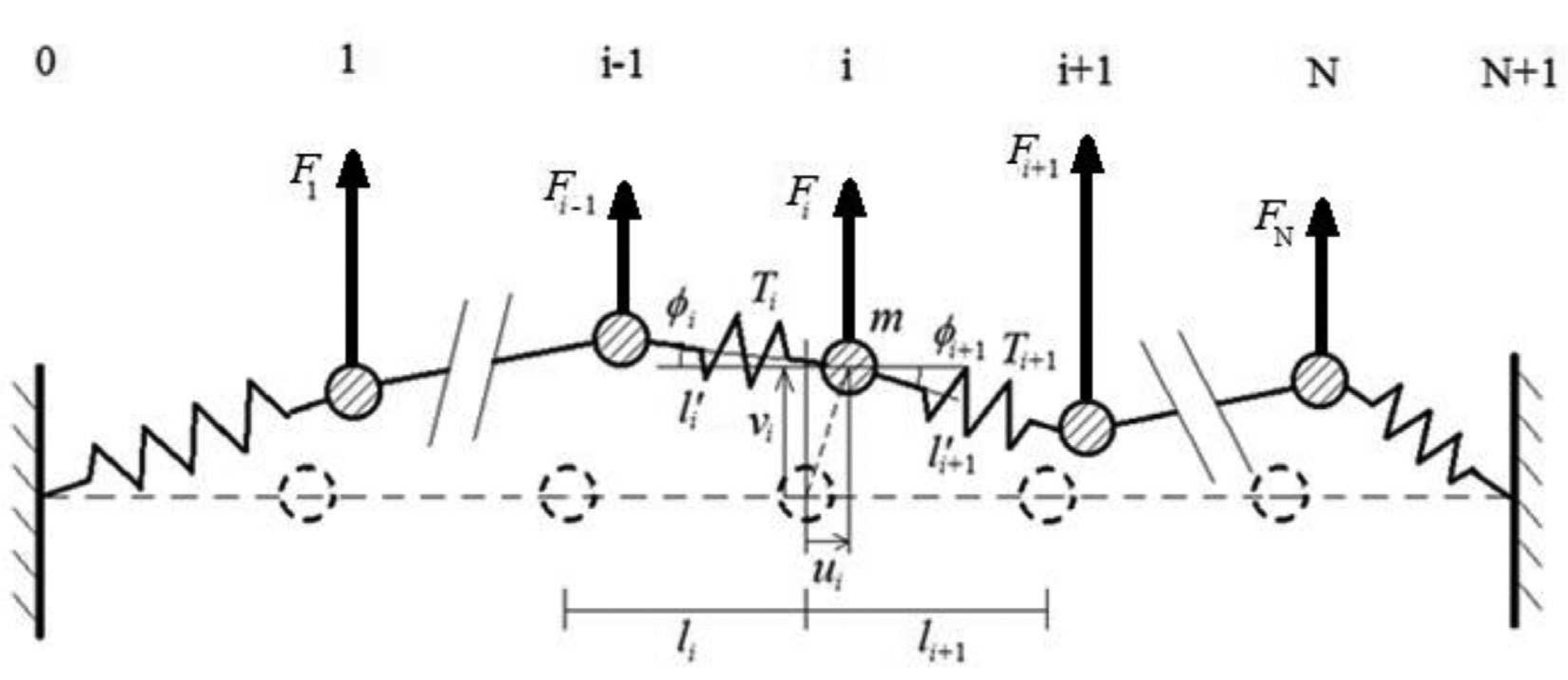
We consider a lattice consisting of N identical particles coupled by identical linear springs (they are un-stretched when the lattice is in the horizontal position) and executing in-plane oscillations (see Figure 1). Fixed boundary conditions and dissipative terms are imposed, and the transverse harmonic forces are also applied. The equations of motion can be expressed as follows,

$$\begin{array}{ccc}{\displaystyle m\frac{d^2{u}_i}{d{t}^2}+\left(T_i-\xi \frac{d{ϵ}_i}{dt}\right)cos{\varphi }_i-\left(T_{i+1}-\xi \frac{d{ϵ}_{i+1}}{dt}\right)cos{\varphi }_{i+1}}\hfill & =\hfill & 0\hfill \\ {\displaystyle m\frac{d^2{v}_i}{d{t}^2}+\left(T_i-\xi \frac{d{ϵ}_i}{dt}\right)sin{\varphi }_i-\left(T_{i+1}-\xi \frac{d{ϵ}_{i+1}}{dt}\right)sin{\varphi }_{i+1}-F_i}\hfill & =\hfill & 0\hfill \end{array}$$

(1)

with $u_i,v_i$ being the longitudinal and transversal displacements of the i-th particle, respectively, ${\varphi }_i$ the angle between the i-th spring and the horizontal direction, $\xi$ the damping coefficient, ${ϵ}_i=l_i^{\prime }-l_i$ the deformation of the i-th spring, $F_i$ the exciting transverse force and m the mass of each particle of the lattice. The tensile forces are proportional to the deformations of the springs, and considering the geometry of the deformed state of the lattice (see Figure 1), one may write:

$$\begin{array}{ccc}{\displaystyle T_i}\hfill & =\hfill & k(l_i^{\prime }-l_i),\hfill \\ {\displaystyle {ϵ}_i=l_i^{\prime }-l_i}\hfill & =\hfill & {[{(v_i-v_{i-1})}^2+{(l_i+u_i-u_{i-1})}^2]}^{1/2}-l_i\hfill \end{array}$$

with $l_i$ being the equilibrium length of the i-th spring (each spring has the same length) and k the linear stiffness coefficient of each coupling spring. Introducing ${\delta }_i={ϵ}_i/l_i$, $s_i=u_i/l_i$, $w_i=v_i/l_i$, $c=\xi /{\left(km\right)}^{1/2}$, where $s_i$ and $w_i$ are the normalized axial and transverse displacements, and the “slow” time scale $\tau ={\left(\frac{k}{m}\right)}^{1/2}t$, Equation (1) can be rewritten in normalized form:

$$\begin{array}{ccc}{\displaystyle \frac{d^2{s}_i}{d{\tau }^2}}\hfill & =\hfill & {\delta }_{i}cos{\varphi }_i-{\delta }_{i-1}cos{\varphi }_{i-1}+c{\delta }_i^{\prime }cos{\varphi }_i-c{\delta }_{i-1}^{\prime }cos{\varphi }_{i-1}\hfill \\ {\displaystyle \frac{d^2{w}_i}{d{\tau }^2}}\hfill & =\hfill & {\delta }_{i}sin{\varphi }_i-{\delta }_{i-1}sin{\varphi }_{i-1}+c{\delta }_i^{\prime }sin{\varphi }_i-c{\delta }_{i-1}^{\prime }sin{\varphi }_{i-1}+f_i,\hfill \end{array}$$

(2)

where:

$$\begin{array}{ccc}\hfill {\displaystyle {\delta }_i}& =\hfill & {[{(w_{i+1}-w_i)}^2+(1+s_{i+1}-s_i)]}^{1/2}-1,\hfill \\ \hfill {\displaystyle {\delta }_i^{\prime }}& =\hfill & \frac{(w_{i+1}-w_i)(w_{i+1}^{\prime }-w_i^{\prime })+(1+s_{i+1}-s_i)(s_{i+1}^{\prime }-s_i^{\prime })}{{[{(w_{i+1}-w_i)}^2+{(1+s_{i+1}-s_i)}^2]}^{1/2}}\hfill \end{array}$$

and:

$$\begin{array}{ccc}\hfill {\displaystyle cos{\varphi }_i}& \hfill =& \frac{1+s_{i+1}-s_i}{{[{(w_{i+1}-w_i)}^2+{(1+s_{i+1}-s_i)}^2]}^{1/2}},\hfill \\ \hfill {\displaystyle sin{\varphi }_i}& \hfill =& \frac{w_{i+1}-w_i}{{[{(w_{i+1}-w_i)}^2+{(1+s_{i+1}-s_i)}^2]}^{1/2}},\hfill \\ \hfill {\displaystyle f_i}& \hfill =& \frac{F_i}{k}.\hfill \end{array}$$

The normalized system (2) is referred to as the “exact lattice” in the following sections.

According to the previous research [1], when we introduce this system (2) without extra transverse force and damping terms, an interesting feature is that in the low energy limit and under the assumption that the axial displacements are assumed to be an order of magnitude smaller compared to the transverse ones, it was shown that, correct to the leading order of approximation, the transverse oscillations decouple from the axial ones and are governed by the following reduced system of equations for predominantly transverse oscillations of the particles:

$$\begin{array}{c}{\displaystyle \frac{d^2{w}_i}{d{\tau }^2}+2^{-1}{(N+1)}^{-1}\sum _{q=0}^N{(w_{q+1}-w_q)}^2(2w_i-w_{i+1}-w_{i-1})=0,}\\ {\displaystyle i=1,\cdots ,N,w_0\left(0\right)=w_{N+1}\left(0\right)=0.}\end{array}$$

(3)

Then, the nearly linear axial oscillations are driven by the transverse responses (see [1,2] for more details). Therefore, we focus our analysis like in [1] just on Equation (3), which presents a low-energy nonlinear acoustic vacuum, because in the absence of linear terms, it possesses zero speed of sound in the context of classical linear acoustics. What is more, it is notable that the existence of the strongly nonlocal multiplier $2^{-1}{(N+1)}^{-1}{\sum }_{q=0}^N{(w_{q+1}-w_q)}^2$ indicates that the response of each particle is dependent (and hence, it is coupled) on the responses of all other particles. Equation (3) admits N exact nonlinear standing waves, or nonlinear normal modes (NNMs), in the form:

$$w_i\left(\tau \right)=A_p\left(\tau \right)sin\frac{\pi pi}{N+1},i=1,\cdots ,N$$

for the p-th NNM, $1\le p\le N$, where $A_p\left(\tau \right)$ denotes the p-th modal amplitude. These, by construction, are mutually orthogonal, and there are no other NNMs in this system, nor any NNM bifurcations [1]. Substituting this NNM ansatz into Equation (3) yields a set of N uncoupled nonlinear equations governing the time-dependent amplitudes of the NNMs:

$$A_p^{″}\left(\tau \right)+(1/4){\omega }_p^4{A}_p^3\left(\tau \right)=0$$

with:

$${\omega }_p=2sin\frac{\pi p}{2(N+1)},$$

which is the p-th natural frequency of the corresponding linear system Equation (3) and the prime denoting differentiation with respect to $\tau$. The exciting force, which is applied on each particle in the transverse direction, is expressed as:

$$f_i=F_{p}cos{\omega }_p\tau sin\frac{pi\pi }{n+1}$$

where $i=1,\cdots ,N$, for the p-th NNM, $1\le p\le N$, and this exciting force includes NNMs in the form $sin\frac{pi\pi }{n+1},i=1,\cdots ,N,$ for the p-th NNM, $1\le p\le N$ and the p-th natural linear frequency ${\omega }_p$.

The frequency of the p-th NNM is tunable with the force and energy, and it also paves the way for nonlinear resonances between NNMs widely separated in the nonlinear spectrum, given that their energies tune their frequencies to satisfy certain rational relationships.

Summarizing, we can write (3) as:

$$\frac{d^{2}w}{d{\tau }^2}+2^{-1}{(N+1)}^{-1}\langle Mw,w\rangle Mw=0,$$

where $w=[w_1,\cdots ,w_N]\in {\mathbb{R}}^N$, M is a symmetric matrix given by

$$M=\left(\begin{array}{ccccc}2& -1& 0& \cdots & 0\\ -1& 2& -1& \cdots & 0\\ ⋮& ⋮& ⋮& ⋮& ⋮\\ 0& \cdots & -1& 2& -1\\ 0& \cdots & 0& -1& 2\end{array}\right)$$

and $\langle ·,·\rangle$ is the standard scalar product on ${\mathbb{R}}^N$. The eigenvectors of M are ${\underline{\varphi }}_p=[sin\frac{p\pi }{N+1},\cdots ,sin\frac{pN\pi }{N+1}]$ with the corresponding eigenvalues ${\omega }_p^2$, $1\le p\le N$. Moreover, it holds (see [4], p. 37):

$$\begin{array}{c}\langle {\underline{\varphi }}_p,{\underline{\varphi }}_p\rangle ={\displaystyle \sum _{i=1}^N}{sin}^2\frac{pi\pi }{N+1}=\frac{N+1}{2},\\ \langle {\underline{\varphi }}_p,{\underline{\varphi }}_k\rangle ={\displaystyle \sum _{i=1}^N}sin\frac{pi\pi }{N+1}sin\frac{ki\pi }{N+1}\\ =\frac{1}{2}{\displaystyle \sum _{i=1}^N}\left(cos\frac{(p-k)i\pi }{N+1}-cos\frac{(p+k)i\pi }{N+1}\right)=0,p\ne k.\end{array}$$

The forced (3) has the form:

$$\frac{d^{2}w}{d{\tau }^2}+2^{-1}{(N+1)}^{-1}\langle Mw,w\rangle Mw=\sum _{p=1}^N{F}_{p}cos{\omega }_p\tau {\underline{\varphi }}_p.$$

(4)

Therefore, considering the basis ${\{{\underline{\varphi }}_p\}}_{p=1}^N$ of ${\mathbb{R}}^N$, we take $w\left(\tau \right)={\sum }_{p=1}^N{C}_p\left(\tau \right){\underline{\varphi }}_p$ in (4) to get:

$$C_p^{″}\left(\tau \right)+\frac{1}{4}\left(\sum _{i=1}^N{C}_i^2\left(\tau \right){\omega }_i^2\right){\omega }_p^2{C}_p\left(\tau \right)=F_{p}cos{\omega }_p\tau ,1\le p\le N.$$

(5)

Next, applying the coordinate transformation to (5):

$$A_p\left(\tau \right)=\frac{{\omega }_p}{2}{C}_p\left(\tau \right),1\le p\le N,$$

we get:

$$A_p^{″}\left(\tau \right)+\left(\sum _{i=1}^N{A}_i^2\left(\tau \right)\right){\omega }_p^2{A}_p\left(\tau \right)=\frac{F_p{\omega }_p}{2}cos{\omega }_p\tau ,1\le p\le N.$$

3. Two-Mode System

In this paper, we consider just two modes: k and p, so we study the system:

$$\begin{array}{ccc}{\displaystyle A_k^{″}\left(\tau \right)+[A_k^2\left(\tau \right)+A_p^2\left(\tau \right)]{\omega }_k^2{A}_k\left(\tau \right)+ϵ{\mu }_{1}cos\left({\omega }_k\tau \right)}\hfill & =\hfill & 0\hfill \\ {\displaystyle A_p^{″}\left(\tau \right)+[A_k^2\left(\tau \right)+A_p^2\left(\tau \right)]{\omega }_p^2{A}_p\left(\tau \right)+ϵ{\mu }_{2}cos\left({\omega }_p\tau \right)}\hfill & =\hfill & 0,\hfill \end{array}$$

(6)

for $ϵ\ne 0$ small and parameters ${\mu }_1$, ${\mu }_2$. Using the transformation:

$$\begin{array}{ccc}{\displaystyle {\psi }_1\left(\tau \right)}\hfill & =\hfill & A_k^{\prime }\left(\tau \right)+j\Omega A_k\left(\tau \right)\equiv {\zeta }_1\left(\tau \right)e^{j\Omega \tau }\hfill \\ {\displaystyle {\psi }_2\left(\tau \right)}\hfill & =\hfill & A_p^{\prime }\left(\tau \right)+j\Omega A_p\left(\tau \right)\equiv {\zeta }_2\left(\tau \right)e^{j\Omega \tau },\hfill \end{array}$$

and performing an averaging approach like in [1], Equation (6) is modified to the form:

$$\begin{array}{ccc}{\displaystyle {\zeta }_1^{\prime }+\frac{j\Omega }{2}{\zeta }_1-\frac{j{\omega }_k^2}{8{\Omega }^3}({\zeta }_2^2{\zeta }_1^{\ast }+2|{\zeta }_2{|}^2{\zeta }_1+3|{\zeta }_1{|}^2{\zeta }_1)+ϵ{\mu }_{1}cos\left({\omega }_k\tau \right)e^{-j\Omega \tau }}\hfill & =\hfill & 0\hfill \\ {\displaystyle {\zeta }_2^{\prime }+\frac{j\Omega }{2}{\zeta }_2-\frac{j{\omega }_p^2}{8{\Omega }^3}({\zeta }_1^2{\zeta }_2^{\ast }+2|{\zeta }_1{|}^2{\zeta }_2+3|{\zeta }_2{|}^2{\zeta }_2)+ϵ{\mu }_{2}cos\left({\omega }_p\tau \right)e^{-j\Omega \tau }}\hfill & =\hfill & 0.\hfill \end{array}$$

Introducing ${\zeta }_i=a_i{e}^{j{\beta }_i}$ and $\Delta ={\beta }_2-{\beta }_1$, we get:

$$\begin{array}{ccc}\hfill {\displaystyle a_1^{\prime }+\frac{{\omega }_k^2}{8{\Omega }^3}{a}_2^2{a}_{1}sin2\Delta +ϵ{\mu }_{1}cos\left({\omega }_k\tau \right)cos(\Omega \tau +{\beta }_1)}& \hfill =& 0\hfill \\ \hfill {\displaystyle a_2^{\prime }-\frac{{\omega }_p^2}{8{\Omega }^3}{a}_1^2{a}_{2}sin2\Delta +ϵ{\mu }_{2}cos\left({\omega }_p\tau \right)cos(\Omega \tau +{\beta }_1+\Delta )}& \hfill =& 0\hfill \\ \hfill {\displaystyle {\Delta }^{\prime }-\frac{{\omega }_p^2}{8{\Omega }^3}(3a_2^2+a_1^{2}cos2\Delta +2a_1^2)+\frac{{\omega }_k^2}{8{\Omega }^3}(3a_1^2+a_2^{2}cos2\Delta +2a_2^2)}\\ \hfill {\displaystyle -\frac{ϵ{\mu }_2}{a_2}cos\left({\omega }_p\tau \right)sin(\Omega \tau +{\beta }_1+\Delta )+\frac{ϵ{\mu }_1}{a_1}cos\left({\omega }_k\tau \right)sin(\Omega \tau +{\beta }_1)}& \hfill =& 0\hfill \end{array}$$

(7)

where we consider ${\beta }_1$ as a constant parameter. Now, by introducing the coordinate transformations $a_1=(\frac{\rho }{{\omega }_p})sin\theta$ and $a_2=(\frac{\rho }{{\omega }_k})cos\theta$ into Equation (7), we get:

$$\begin{array}{c}\hfill {\displaystyle {\rho }^{\prime }=-ϵ{\mu }_1{\omega }_{p}sin\theta cos\left({\omega }_k\tau \right)cos(\Omega \tau +{\beta }_1)-ϵ{\mu }_2{\omega }_{k}cos\theta cos\left({\omega }_p\tau \right)cos(\Omega \tau +\Delta +{\beta }_1)}\\ \hfill {\displaystyle {\theta }^{\prime }+\frac{{\rho }^2}{16{\Omega }^3}sin2\theta sin2\Delta +ϵ{\mu }_1{\omega }_p\frac{cos\theta }{\rho }cos\left({\omega }_k\tau \right)cos(\Omega \tau +{\beta }_1)}\\ \hfill {\displaystyle -ϵ{\mu }_2{\omega }_k\frac{sin\theta }{\rho }cos\left({\omega }_p\tau \right)cos(\Omega \tau +\Delta +{\beta }_1)=0}\\ \hfill {\displaystyle {\Delta }^{\prime }-\frac{{\rho }^2}{8{\Omega }^3}\left[\frac{3{\omega }_p^2}{{\omega }_k^2}{cos}^2\theta -\frac{3{\omega }_k^2}{{\omega }_p^2}{sin}^2\theta -cos2\theta (2+cos2\Delta )\right]}\\ \hfill {\displaystyle -\frac{ϵ{\mu }_2{\omega }_k}{\rho cos\theta }cos\left({\omega }_p\tau \right)sin(\Omega \tau +\Delta +{\beta }_1)+\frac{ϵ{\mu }_1{\omega }_p}{\rho sin\theta }cos\left({\omega }_k\tau \right)sin(\Omega \tau +{\beta }_1)=0.}\end{array}$$

In the rest of the paper, we assume ${\omega }_p={\omega }_k=P$ and $\Omega =kP$ for a natural number k, so we study the periodically-perturbed system:

$$\begin{array}{c}\hfill {\displaystyle {\rho }^{\prime }=-ϵ{\mu }_{1}sin\theta cos\left(P\tau \right)cos(kP\tau +{\beta }_1)-ϵ{\mu }_{2}cos\theta cos\left(P\tau \right)cos(kP\tau +\Delta +{\beta }_1)}\\ \hfill {\displaystyle {\theta }^{\prime }+\frac{{\rho }^2}{16k^3{P}^3}sin2\theta sin2\Delta +ϵ{\mu }_1\frac{cos\theta }{\rho }cos\left(P\tau \right)cos(kP\tau +{\beta }_1)}\\ \hfill {\displaystyle -ϵ{\mu }_2\frac{sin\theta }{\rho }cos\left(P\tau \right)cos(kP\tau +\Delta +{\beta }_1)=0}\\ \hfill {\displaystyle {\Delta }^{\prime }-\frac{{\rho }^2}{4k^3{P}^3}cos2\theta {sin}^2\Delta +\frac{ϵ{\mu }_1}{\rho sin\theta }cos\left(P\tau \right)sin(kP\tau +{\beta }_1)}\\ \hfill {\displaystyle -\frac{ϵ{\mu }_2}{\rho cos\theta }cos\left(P\tau \right)sin(kP\tau +\Delta +{\beta }_1)=0}\end{array}$$

(8)

where we scaled $P{\mu }_i\leftrightarrow {\mu }_i$, $i=1,2$. We may suppose:

$${\mu }_1^2+{\mu }_2^2=1.$$

First, consider the unperturbed case where $ϵ=0$, so the system:

$$\begin{array}{c}\hfill {\displaystyle {\rho }^{\prime }=0}\\ \hfill {\displaystyle {\theta }^{\prime }+\frac{{\rho }^2}{16k^3{P}^3}sin2\theta sin2\Delta =0}\\ \hfill {\displaystyle {\Delta }^{\prime }-\frac{{\rho }^2}{4k^3{P}^3}cos2\theta {sin}^2\Delta =0.}\end{array}$$

(9)

By introducing the temporal variable ${\tau }_2=\frac{{\rho }^2}{8k^3{P}^3}\tau$ in Equation (9), we get:

$$\begin{array}{ccc}\hfill {\displaystyle \frac{d\theta }{d{\tau }_2}}& \hfill =& \hfill -\frac{1}{2}sin2\theta sin2\Delta \\ \hfill {\displaystyle \frac{d\Delta }{d{\tau }_2}}& \hfill =& \hfill 2cos2\theta {sin}^2\Delta \end{array}$$

(10)

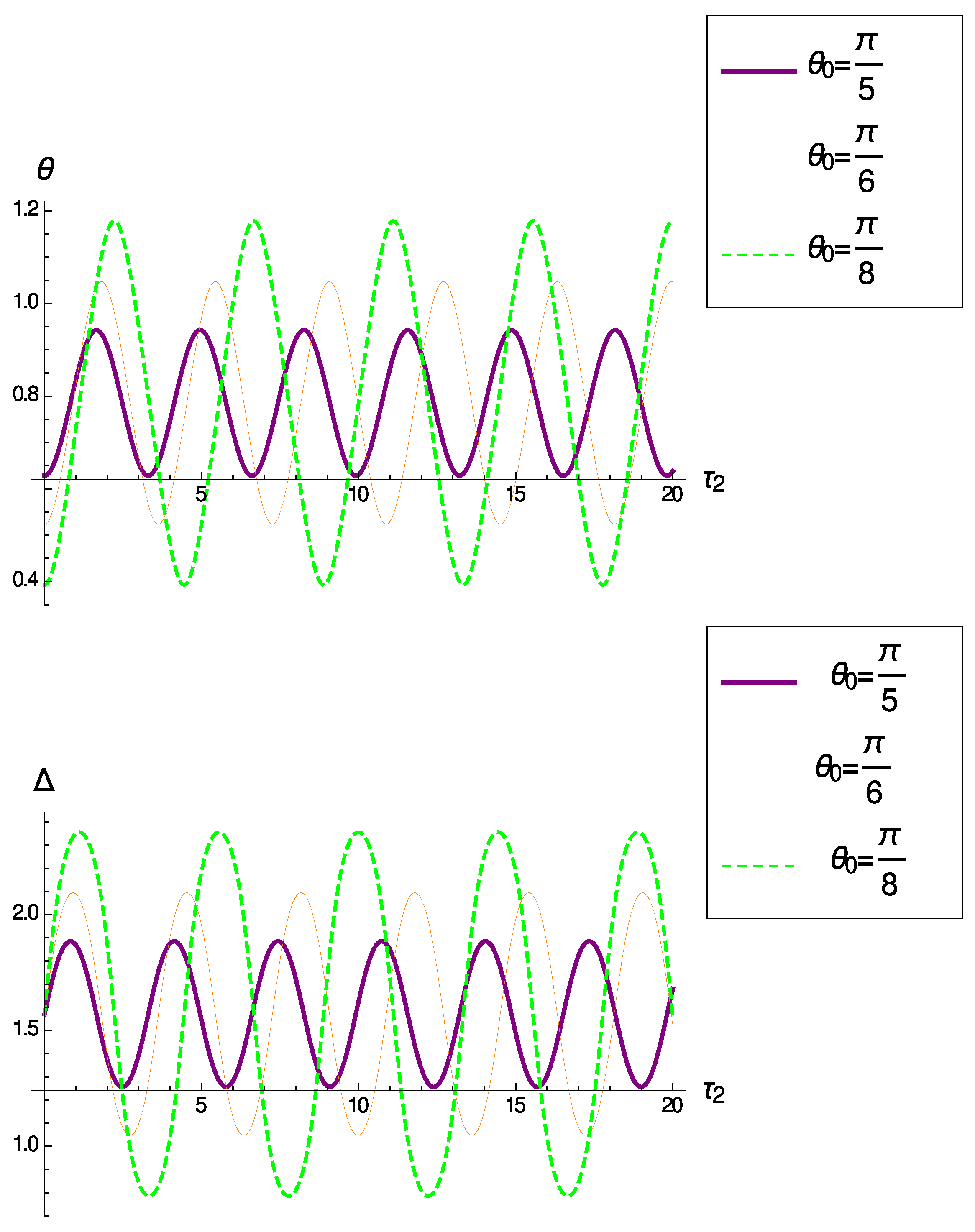
which is fully integrable and gives us the first integral $I=sin2\theta sin\Delta =K=const.$ of the degenerate slow flow. If we consider the following initial conditions: $\theta \left(0\right)={\theta }_0$, where $0<{\theta }_0<\frac{\pi }{4}$ and $\Delta \left(0\right)=\pi /2$, then we get $K=sin2{\theta }_0\in (0,1)$. To find exact solutions of (10), we first derive:

$$\begin{array}{c}\frac{d{\tau }_2}{d\theta }=-\frac{2}{sin2\theta sin2\Delta }=-\frac{1}{Kcos\Delta }=\frac{1}{K\sqrt{1-{sin}^2\Delta }}\\ =\frac{1}{K\sqrt{1-\frac{K^2}{{sin}^{2}2\theta }}}=\frac{1}{K}\frac{sin2\theta }{\sqrt{{sin}^{2}2\theta -K^2}},\end{array}$$

for ${\tau }_2>0$ small, since (10) gives $0<\theta <\frac{\pi }{2}$, $0<\Delta <\pi$ (see Figure 2) and $\frac{d\Delta }{d{\tau }_2}\left(0\right)=2cos2{\theta }_0>0$, so for ${\tau }_2>0$ small, we have $\Delta \left({\tau }_2\right)>\frac{\pi }{2}$.

By using the formula in [4] ((2.599.4) p. 205), we obtain:

$${\tau }_2={\int }_{{\theta }_0}^{\theta }\frac{1}{K}\frac{sin2\theta }{\sqrt{{sin}^{2}2\theta -K^2}}d\theta =\frac{1}{2K}\left(\frac{\pi }{2}-{sin}^{-1}\left(\frac{cos2\theta }{\sqrt{1-K^2}}\right)\right),$$

which gives:

$$\theta \left({\tau }_2\right)=\frac{1}{2}{cos}^{-1}\left(\sqrt{1-K^2}cos\left(2K{\tau }_2\right)\right),$$

(11)

recalling $0<\theta <\frac{\pi }{2}$. Of course, Formula (11) holds for all ${\tau }_2$, not just for small positive ones. Next, using (10) and (11), we have:

$$\frac{d\Delta }{d{\tau }_2}=2\sqrt{1-K^2}cos\left(2K{\tau }_2\right){sin}^2\Delta ,$$

which can be easily solved to arrive at:

$$\Delta \left({\tau }_2\right)=\pi -{cot}^{-1}\left(\frac{\sqrt{1-K^2}}{K}sin\left(2K{\tau }_2\right)\right).$$

Hence, the exact solution of the system (10) is given as:

$$\begin{array}{c}\theta \left({\tau }_2\right)=\frac{1}{2}{cos}^{-1}\left(\sqrt{1-K^2}cos\left(2K{\tau }_2\right)\right)\\ \Delta \left({\tau }_2\right)=\pi -{cot}^{-1}\left(\frac{\sqrt{1-K^2}}{K}sin\left(2K{\tau }_2\right)\right)\end{array}$$

where the period is:

$$T\left({\theta }_0\right)=\frac{2}{K}{\int }_{{\theta }_0}^{\frac{\pi }{2}-{\theta }_0}\frac{d\theta }{{\left(1-\frac{{sin}^{2}2{\theta }_0}{{sin}^{2}2\theta }\right)}^{1/2}}=\frac{\pi }{K}.$$

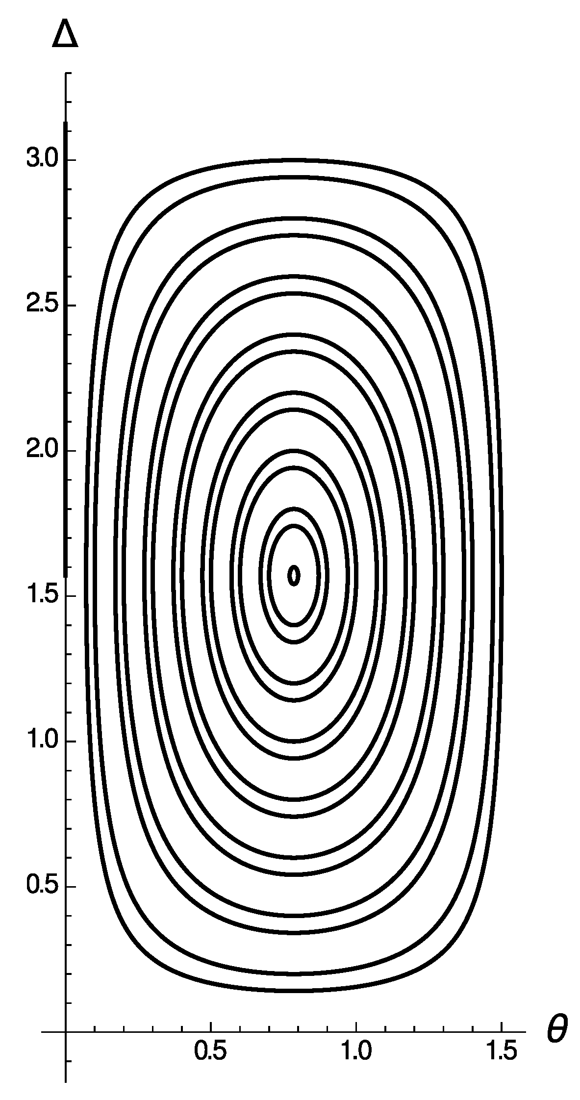
It is easy to verify the following symmetry property (see Figure 3):

$$\Delta \left({\tau }_2+\frac{T}{2}\right)=\pi -\Delta \left({\tau }_2\right),\theta \left({\tau }_2+\frac{T}{2}\right)=\frac{\pi }{2}-\theta \left({\tau }_2\right).$$

Summarizing, the exact solution of the unperturbed (9) is the following:

$$\begin{array}{c}\rho \left(\tau \right)=const.\\ \theta \left(\tau \right)=\frac{1}{2}{cos}^{-1}\left(\sqrt{1-K^2}cos\left(\frac{K{\rho }^2}{4k^3{P}^3}\tau \right)\right)\\ \Delta \left(\tau \right)=\pi -{cot}^{-1}\left(\frac{\sqrt{1-K^2}}{K}sin\left(\frac{K{\rho }^2}{4k^3{P}^3}\tau \right)\right)\end{array}$$

with the period:

$$T=\frac{8k^3{P}^3\pi }{K{\rho }^2}.$$

Consequently, for any:

$$\rho >2k{P}^2\sqrt{k},$$

taking:

$$K\left(\rho \right)=\frac{4k^3{P}^4}{{\rho }^2}\in (0,1),$$

Equation (9) has the $T=2\pi /P$-periodic solution:

$$\begin{array}{c}\theta (\rho ,\tau )=\frac{1}{2}{cos}^{-1}\left(\frac{\sqrt{{\rho }^4-16k^6{P}^8}}{{\rho }^2}cos\left(P\tau \right)\right)\\ \Delta (\rho ,\tau )=\pi -{cot}^{-1}\left(\frac{\sqrt{{\rho }^4-16k^6{P}^8}}{4k^3{P}^4}sin\left(P\tau \right)\right).\end{array}$$

(12)

4. Melnikov Analysis for Periodic Oscillations

Writing (8) as:

$$\begin{array}{c}\hfill {\displaystyle {\theta }^{\prime }+\frac{{\rho }^2}{16k^3{P}^3}sin2\theta sin2\Delta =ϵ{\rho }^{-1}{g}_1(\rho ,\theta ,\Delta ,\tau )}\\ \hfill {\displaystyle {\Delta }^{\prime }-\frac{{\rho }^2}{4k^3{P}^3}cos2\theta {sin}^2\Delta =ϵ{\rho }^{-1}{g}_2(\rho ,\theta ,\Delta ,\tau )}\\ \hfill {\displaystyle {\rho }^{\prime }=ϵg_3(\rho ,\theta ,\Delta ,\tau )}\end{array}$$

and using [5], (3.5.11), p. 111, with $\alpha =0$, and [6], Lemma 2.5, p. 283, we compute the Melnikov function:

$$M({\beta }_1,\rho )=\left(M_1({\beta }_1,\rho ),M_2({\beta }_1,\rho )\right)$$

as:

$$\begin{array}{c}{M}_1({\beta }_1,\rho )={\int }_0^T\left(\frac{\partial I}{\partial \theta }{\rho }^{-1}{g}_1+\frac{\partial I}{\partial \Delta }{\rho }^{-1}{g}_2-\frac{\partial I}{\partial \theta }\frac{\partial \theta }{\partial \rho }{g}_3-\frac{\partial I}{\partial \Delta }\frac{\partial \Delta }{\partial \rho }{g}_3\right)d\tau \\ ={\int }_0^T\left(\frac{\partial I}{\partial \theta }{\rho }^{-1}{g}_1+\frac{\partial I}{\partial \Delta }{\rho }^{-1}{g}_2\right)d\tau -\frac{dK}{d\rho }{\int }_0^T{g}_{3}d\tau \end{array}$$

(13)

since differentiating by $\rho$ the identity:

$$I\left(\theta \right(\rho ,\tau ),\Delta (\rho ,\tau \left)\right)=K\left(\rho \right),$$

we get:

$$\frac{\partial I}{\partial \theta }\frac{\partial \theta }{\partial \rho }+\frac{\partial I}{\partial \Delta }\frac{\partial \Delta }{\partial \rho }=\frac{dK}{d\rho },$$

which is independent of $\tau$, and:

$$M_2({\beta }_1,\rho )={\int }_0^T{g}_{3}d\tau .$$

(14)

Formulas (13) and (14) are similar to [3], (2.7). We are looking for a simple zero of M, which is equivalent to considering:

$$\begin{array}{c}\overline{M}({\beta }_1,\rho )=\left({\overline{M}}_1({\beta }_1,\rho ),{\overline{M}}_2({\beta }_1,\rho )\right)\\ {\overline{M}}_1({\beta }_1,\rho )={\int }_0^T\left(\frac{\partial I}{\partial \theta }{g}_1+\frac{\partial I}{\partial \Delta }{g}_2\right)d\tau ,{\overline{M}}_2({\beta }_1,\rho )={\int }_0^T{g}_{3}d\tau .\end{array}$$

Since:

$$g_i={\mu }_1{g}_{i1}+{\mu }_2{g}_{i2},i=1,2,3$$

for:

$$\begin{array}{c}{\displaystyle g_{11}(\rho ,\theta ,\Delta ,\tau )=-cos\theta cos\left(P\tau \right)cos(kP\tau +{\beta }_1)}\hfill \\ {\displaystyle g_{12}(\rho ,\theta ,\Delta ,\tau )=sin\theta cos\left(P\tau \right)cos(kP\tau +\Delta +{\beta }_1)}\hfill \\ {\displaystyle g_{21}(\rho ,\theta ,\Delta ,\tau )=-\frac{cos\left(P\tau \right)}{sin\theta }sin(kP\tau +{\beta }_1)}\hfill \\ {\displaystyle g_{22}(\rho ,\theta ,\Delta ,\tau )=\frac{cos\left(P\tau \right)}{cos\theta }sin(kP\tau +\Delta +{\beta }_1)}\hfill \\ {\displaystyle g_{31}(\rho ,\theta ,\Delta ,\tau )=-sin\theta cos\left(P\tau \right)cos(kP\tau +{\beta }_1)}\hfill \\ {\displaystyle g_{32}(\rho ,\theta ,\Delta ,\tau )=-cos\theta cos\left(P\tau \right)cos(kP\tau +\Delta +{\beta }_1)}\hfill \end{array}$$

we get:

$${\overline{M}}_i({\beta }_1,\rho )={\mu }_1{\overline{M}}_{i1}({\beta }_1,\rho )+{\mu }_2{\overline{M}}_{i2}({\beta }_1,\rho ),i=1,2,$$

for

$${\overline{M}}_{1j}({\beta }_1,\rho )={\int }_0^T\left(\frac{\partial I}{\partial \theta }{g}_{1j}+\frac{\partial I}{\partial \Delta }{g}_{2j}\right)d\tau ,{\overline{M}}_{2j}({\beta }_1,\rho )={\int }_0^T{g}_{3j}d\tau ,j=1,2.$$

To solve:

$${\mu }_1{\overline{M}}_{i1}({\beta }_1,\rho )+{\mu }_2{\overline{M}}_{i2}({\beta }_1,\rho )=0,i=1,2,$$

we first solve the scalar equation:

$$\tilde{M}({\beta }_1,\rho )={\overline{M}}_{11}({\beta }_1,\rho ){\overline{M}}_{22}({\beta }_1,\rho )-{\overline{M}}_{12}({\beta }_1,\rho ){\overline{M}}_{21}({\beta }_1,\rho )=0$$

(15)

to get its root ${\beta }_{1,0}$ and ${\rho }_0$. Then, we look for ${\mu }_{1,0}$ and ${\mu }_{2,0}$ with ${\mu }_{1,0}^2+{\mu }_{2,0}^2=1$ such that:

$$\begin{array}{c}{\mu }_{1,0}{\overline{M}}_{i1}({\beta }_{1,0},{\rho }_0)+{\mu }_{2,0}{\overline{M}}_{i2}({\beta }_{1,0},{\rho }_0)=0,i=1,2\\ det\left(\begin{array}{c}{\mu }_{1,0}\nabla {\overline{M}}_{11}{({\beta }_{1,0},{\rho }_0)}^{\top }+{\mu }_{2,0}\nabla {\overline{M}}_{12}{({\beta }_{1,0},{\rho }_0)}^{\top }\\ {\mu }_{1,0}\nabla {\overline{M}}_{21}{({\beta }_{1,0},{\rho }_0)}^{\top }+{\mu }_{2,0}\nabla {\overline{M}}_{22}{({\beta }_{1,0},{\rho }_0)}^{\top }\end{array}\right)\ne 0.\end{array}$$

(16)

Summarizing, we have the following result.

Theorem 1.

If there are ${\beta }_{1,0}\in [0,2\pi )$, ${\rho }_0$ satisfying (15), ${\mu }_{1,0}$ and ${\mu }_{2,0}$ with ${\mu }_{1,0}^2+{\mu }_{2,0}^2=1$ solving (16), then for any ${\mu }_1$ near ${\mu }_{1,0}$ and ${\mu }_2$ near ${\mu }_{2,0}$ with ${\mu }_1^2+{\mu }_2^2=1$ and $ϵ\ne 0$ small, there are ${\beta }_1\left(ϵ\right)$ near ${\beta }_{1,0}$ and $\rho \left(ϵ\right)$ near ${\rho }_0$ such that (8) with ${\beta }_1={\beta }_1\left(ϵ\right)$ and $\rho =\rho \left(ϵ\right)$ has a $T=2\pi /P$-periodic solution near (12) with $\rho =\rho \left(ϵ\right)$.

Note:

$$\begin{array}{c}{\overline{M}}_{11}({\beta }_1,\rho )=-{\int }_0^T(2cos\left(2\theta (\rho ,\tau )\right)sin\Delta (\rho ,\tau )cos\theta (\rho ,\tau )cos\left(P\tau \right)cos(kP\tau +{\beta }_1)\\ +2cos\theta (\rho ,\tau )cos\Delta (\rho ,\tau )cos\left(P\tau \right)sin(kP\tau +{\beta }_1)\left)\right)d\tau \\ {\overline{M}}_{12}({\beta }_1,\rho )={\int }_0^T(2cos\left(2\theta (\rho ,\tau )\right)sin\Delta (\rho ,\tau )sin\theta (\rho ,\tau )cos\left(P\tau \right)cos(kP\tau +\Delta (\rho ,\tau )+{\beta }_1)\\ +2sin\theta (\rho ,\tau )cos\Delta (\rho ,\tau )cos\left(P\tau \right)sin(kP\tau +\Delta (\rho ,\tau )+{\beta }_1))d\tau \\ {\overline{M}}_{21}({\beta }_1,\rho )=-{\int }_0^{T}sin\theta (\rho ,\tau )cos\left(P\tau \right)cos(kP\tau +{\beta }_1)d\tau \\ {\overline{M}}_{22}({\beta }_1,\rho )=-{\int }_0^{T}cos\theta (\rho ,\tau )cos\left(P\tau \right)cos(kP\tau +\Delta (\rho ,\tau )+{\beta }_1)d\tau .\end{array}$$

Next, taking $\rho \to \infty$ in (12), we obtain:

$$\begin{array}{c}\theta (\infty ,\tau )=\left\{\begin{array}{c}{\displaystyle \frac{P\tau }{2}\tau \in \left[0,\frac{\pi }{P}\right],}\hfill \\ {\displaystyle \pi -\frac{P\tau }{2}\tau \in \left[\frac{\pi }{P},\frac{2\pi }{P}\right],}\hfill \end{array}\right.\\ \Delta (\infty ,\tau )=\left\{\begin{array}{c}{\displaystyle \pi \tau \in \left(0,\frac{\pi }{P}\right),}\hfill \\ {\displaystyle 0\tau \in \left(\frac{\pi }{P},\frac{2\pi }{P}\right),}\hfill \\ {\displaystyle \frac{\pi }{2}\tau \in \left\{0,\frac{\pi }{P},\frac{2\pi }{P}\right\},}\hfill \end{array}\right.\\ \frac{\partial \theta }{\partial \rho }(\infty ,\tau )=0,\frac{\partial \Delta }{\partial \rho }(\infty ,\tau )=0.\end{array}$$

(17)

Hence:

$$\begin{array}{c}{\overline{M}}_{11}({\beta }_1,\infty )={\int }_0^{\frac{2\pi }{P}}2cos\frac{P\tau }{2}cos\left(P\tau \right)sin(kP\tau +{\beta }_1)d\tau \\ =\frac{16k(4k^2-5)cos{\beta }_1}{(16k^4-40k^2+9)P}\\ {\overline{M}}_{12}({\beta }_1,\infty )={\int }_0^{\frac{2\pi }{P}}2sin\frac{P\tau }{2}cos\left(P\tau \right)sin(kP\tau +{\beta }_1))d\tau \\ =-\frac{8(4k^2+3)sin{\beta }_1}{(16k^4-40k^2+9)P}\\ {\overline{M}}_{21}({\beta }_1,\infty )=-{\int }_0^{\frac{2\pi }{P}}sin\frac{P\tau }{2}cos\left(P\tau \right)cos(kP\tau +{\beta }_1)d\tau \\ =\frac{4(4k^2+3)cos{\beta }_1}{(16k^4-40k^2+9)P}\\ {\overline{M}}_{22}({\beta }_1,\infty )={\int }_0^{\frac{2\pi }{P}}cos\frac{P\tau }{2}cos\left(P\tau \right)cos(kP\tau +{\beta }_1)d\tau \\ =-\frac{8k(4k^2-5)sin{\beta }_1}{(16k^4-40k^2+9)P}.\end{array}$$

Then, (15) gives as $\rho \to \infty$,

$$\tilde{M}({\beta }_1,\infty )=-\frac{16sin2{\beta }_1}{(4k^2-9)P^2}$$

with asymptotic solutions ${\beta }_{1,0}^{\infty }$ satisfying either $sin{\beta }_{1,0}^{\infty }=0$ or $cos{\beta }_{1,0}^{\infty }=0$. The asymptotic equation of (16) is as follows:

$$\begin{array}{c}0={\mu }_{1,0}{\overline{M}}_{11}({\beta }_{1,0}^{\infty },\infty )+{\mu }_{2,0}{\overline{M}}_{12}({\beta }_{1,0}^{\infty },\infty )\\ ={\mu }_{1,0}\frac{16k(4k^2-5)cos{\beta }_{1,0}^{\infty }}{(16k^4-40k^2+9)P}-{\mu }_{2,0}\frac{8(4k^2+3)sin{\beta }_{1,0}^{\infty }}{(16k^4-40k^2+9)P},\end{array}$$

which has solutions: ${\mu }_{1,0}^{\infty }=0$ and ${\mu }_{2,0}^{\infty }=\pm 1$ when $sin{\beta }_{1,0}^{\infty }=0$ or ${\mu }_{1,0}^{\infty }=\pm 1$ and ${\mu }_{2,0}^{\infty }=0$ when $cos{\beta }_{1,0}^{\infty }=0$. However, $\frac{\partial {\overline{M}}_{ij}}{\partial \rho }({\beta }_1,\infty )=0$ for $i,j\in \{1,2\}$, so Theorem 1 cannot be applied directly. Note we consider just the first asymptotic equation of (16), since the second one is a scalar multiple of the first one.

On the other hand, following the method of [5], p. 111, we get the following result.

Corollary 1.

For any $\rho >0$ sufficiently large and $ϵ\ne 0$ sufficiently small, there is ${\mu }_1(\rho ,ϵ)$, ${\mu }_2(\rho ,ϵ)$ with ${\mu }_1^2(\rho ,ϵ)+{\mu }_2^2(\rho ,ϵ)=1$ and ${\beta }_1(\rho ,ϵ)$ such that (8) has a T-periodic solution near (17) for $ϵ\ne 0$ small and either ${\mu }_1(\infty ,0)=0$, ${\mu }_2(\infty ,0)=\pm 1$, $sin{\beta }_1(\infty ,0)=0$ or ${\mu }_1(\infty ,0)=\pm 1$, ${\mu }_2(\infty ,0)=0$, $cos{\beta }_1(\infty ,0)=0$.

Proof. 

The bifurcation equation has the form (see [5], p. 111):

$${\mu }_1{\overline{M}}_{i1}({\beta }_1,\rho )+{\mu }_2{\overline{M}}_{i2}({\beta }_1,\rho )=O\left(ϵ\right),i=1,2,{\mu }_1^2+{\mu }_2^2=1$$

i.e.,

$$sin\Gamma {\overline{M}}_{i1}({\beta }_1,\rho )+cos\Gamma {\overline{M}}_{i2}({\beta }_1,\rho )=O\left(ϵ\right),i=1,2$$

(18)

for ${\mu }_1=sin\Gamma$ and ${\mu }_2=cos\Gamma$. For $\rho =\infty$ and $ϵ=0$, (18) takes the form:

$$\begin{array}{c}\frac{16k(4k^2-5)}{(16k^4-40k^2+9)P}sin\Gamma cos{\beta }_1-\frac{8(4k^2+3)}{(16k^4-40k^2+9)P}cos\Gamma sin{\beta }_1=0\\ \frac{4(4k^2+3)cos{\beta }_1}{(16k^4-40k^2+9)P}sin\Gamma cos{\beta }_1-\frac{8k(4k^2-5)}{(16k^4-40k^2+9)P}cos\Gamma sin{\beta }_1=0.\end{array}$$

(19)

The determinant of (19) is $-\frac{32}{(4k^2-9)P^2}\ne 0$, so (19) has the only solutions:

$$sin{\Gamma }_{\infty }=sin{\beta }_{1,0}^{\infty }=0,cos{\Gamma }_{\infty }=cos{\beta }_{1,0}^{\infty }=0.$$

The determinants of Jacobians of (19) at these zeros are as follows:

$$\begin{array}{c}det\left(\begin{array}{cc}\frac{16k(4k^2-5)}{(16k^4-40k^2+9)P}cos{\Gamma }_{\infty }cos{\beta }_{1,0}^{\infty }& -\frac{8(4k^2+3)}{(16k^4-40k^2+9)P}cos{\Gamma }_{\infty }cos{\beta }_{1,0}^{\infty }\\ \frac{4(4k^2+3)cos{\beta }_{1,0}^{\infty }}{(16k^4-40k^2+9)P}cos{\Gamma }_{\infty }cos{\beta }_{1,0}^{\infty }& -\frac{8k(4k^2-5)}{(16k^4-40k^2+9)P}cos{\Gamma }_{\infty }cos{\beta }_{1,0}^{\infty }\end{array}\right)\\ =-\frac{32{cos}^2{\Gamma }_{\infty }{cos}^2{\beta }_{1,0}^{\infty }}{(4k^2-9)P^2}\ne 0\end{array}$$

and:

$$\begin{array}{c}det\left(\begin{array}{cc}\frac{8(4k^2+3)}{(16k^4-40k^2+9)P}sin{\Gamma }_{\infty }sin{\beta }_{1,0}^{\infty }& -\frac{16k(4k^2-5)}{(16k^4-40k^2+9)P}sin{\Gamma }_{\infty }sin{\beta }_{1,0}^{\infty }\\ \frac{8k(4k^2-5)}{(16k^4-40k^2+9)P}sin{\Gamma }_{\infty }sin{\beta }_{1,0}^{\infty }& -\frac{4(4k^2+3)cos{\beta }_{1,0}^{\infty }}{(16k^4-40k^2+9)P}sin{\Gamma }_{\infty }sin{\beta }_{1,0}^{\infty }\end{array}\right)\\ =\frac{32{sin}^2{\Gamma }_{\infty }{sin}^2{\beta }_{1,0}^{\infty }}{(4k^2-9)P^2}\ne 0,\end{array}$$

respectively. Hence, the zeroes ${\Gamma }_{\infty }$ and ${\beta }_{1,0}^{\infty }$ are simple, so we can apply the implicit function theorem to get the result. The proof is complete. ☐

5. Discussion

Melnikov analysis is applied for the persistence of periodic oscillations for periodically-perturbed systems of ODEs with a slowly-varying variable. The ODEs are obtained from a model of a finite lattice of particles coupled by linear springs under distributed harmonic excitation, which presents a low-energy nonlinear acoustic vacuum (see [1]), but we consider just two modes. We extend the study of [1] to a problem with small exciting harmonic forces. We apply an analytical method based on derivation of Melnikov functions and then on the location of their simple roots. Melnikov functions are derived by using the approach of [3,5] developed for slowly-varying ODEs. Since the Melnikov functions are rather complicated, we follow an asymptotic way for solving the corresponding Melnikov equations. It would be nice to solve these Melnikov equations numerically for finding other simple roots, which is postponed to our next research. These roots determine and locate periodic solutions of the periodically-perturbed systems of ODEs derived from the two-mode low-energy nonlinear acoustic vacuum system. Moreover, our next investigation will be also to consider higher numbers of modes represented by a system of ODEs in (5). The method used will be different from that in this paper, since it will be based on the results of Section 3.3 of [5]. Note that higher modes of (2) were numerically studied in [2], which is another challenge for our study.

References

1. Manevich, L.I.; Vakakis, A.F. Nonlinear oscillatory acoustic vacuum. SIAM J. Appl. Math. 2014, 74, 1742–1762. [Google Scholar] [CrossRef]
2. Zhang, Z.; Manevitch, L.I.; Smirnov, V.; Bergman, L.; Vakakis, A.F. Extreme nonlinear energy exchanges in a geometrically nonlinear lattice oscillating in the plane. J. Mech. Phys. Solids 2018, 110, 1–20. [Google Scholar] [CrossRef]
3. Wiggins, S.; Holmes, P. Periodic orbits in slowly varying oscillators. SIAM J. Math. Anal. 1987, 18, 592–611. [Google Scholar] [CrossRef]
4. Gradshteyn, I.S.; Ryzhik, I.M. Table of Integrals, Series, and Products, 7th ed.; Academic Press: Cambridge, MA, USA, 2007. [Google Scholar]
5. Fečkan, M. Topological Degree Approach to Bifurcation Problems; Springer: Berlin, Germany, 2008. [Google Scholar]
6. Hale, J.K. Ordinary Differential Equations, 2nd ed.; Robert E. Krieger Publishing Company, Inc.: Malabar, FL, USA, 1980. [Google Scholar]
Figure 1. Forced and damped lattice oscillating in the plane (see [2]).
Axioms 07 00069 g001
Figure 2. Top panel: Graph for θ for different initial values of θ 0 . Bottom panel: Graph for Δ for different initial values of θ 0 .
Axioms 07 00069 g002
Figure 3. Orbits in the phase portrait of (10), where ( θ , Δ ) [ 0 , π 2 ] × [ 0 , π ] .
Axioms 07 00069 g003