Decision-Making with Bipolar Neutrosophic TOPSIS and Bipolar Neutrosophic ELECTRE-I

Abstract

Technique for the order of preference by similarity to ideal solution (TOPSIS) and elimination and choice translating reality (ELECTRE) are widely used methods to solve multi-criteria decision making problems. In this research article, we present bipolar neutrosophic TOPSIS method and bipolar neutrosophic ELECTRE-I method to solve such problems. We use the revised closeness degree to rank the alternatives in our bipolar neutrosophic TOPSIS method. We describe bipolar neutrosophic TOPSIS method and bipolar neutrosophic ELECTRE-I method by flow charts. We solve numerical examples by proposed methods. We also give a comparison of these methods.

1. Introduction

The theory of fuzzy sets was introduced by Zadeh [1]. Fuzzy set theory allows objects to be members of the set with a degree of membership, which can take any value within the unit closed interval $[0,1]$. Smarandache [2] originally introduced neutrosophy, a branch of philosophy which examines the origin, nature, and scope of neutralities, as well as their connections with different intellectual spectra. To apply neutrosophic set in real-life problems more conveniently, Smarandache [2] and Wang et al. [3] defined single-valued neutrosophic sets which takes the value from the subset of $[0,1]$. Thus, a single-valued neutrosophic set is an instance of neutrosophic set, and can be used feasibly to deal with real-world problems, especially in decision support. Deli et al. [4] dealt with bipolar neutrosophic sets, which is an extension of bipolar fuzzy sets [5].

Multi-criteria decision making (MCDM) is a process to make an ideal choice that has the highest degree of achievement from a set of alternatives that are characterized in terms of multiple conflicting criteria. Hwang and Yoon [6] developed the TOPSIS method, which is one of the most favorable and effective MCDM methods to solve MCDM problems. In classical MCDM methods, the attribute values and weights are determined precisely. To deal with problems consisting of incomplete and vague information, in 2000 Chen [7] conferred the fuzzy version of TOPSIS method for the first time. Chung and Chu [8] presented fuzzy TOPSIS method under group decision for facility location selection problem. Hadi et al. [9] proposed the fuzzy inferior ratio method for multiple attribute decision making problems. Joshi and Kumar [10] discussed the TOPSIS method based on intuitionistic fuzzy entropy and distance measure for multi criteria decision making. A comparative study of multiple criteria decision making methods under stochastic inputs is described by Kolios et al. [11]. Akram et al. [12,13,14] considered decision support systems based on bipolar fuzzy graphs. Applications of bipolar fuzzy sets to graphs have been discussed in [15,16]. Faizi et al. [17] presented group decision making for hesitant fuzzy sets based on characteristic objects method. Recently, Alghamdi et al. [18] have studied multi-criteria decision-making methods in bipolar fuzzy environment. Dey et al. [19] considered TOPSIS method for solving the decision making problem under bipolar neutrosophic environment.

On the other hand, the ELECTRE is one of the useful MCDM methods. This outranking method was proposed by Benayoun et al. [20], which was later referred to as ELECTRE-I method. Different versions of ELECTRE method have been developed as ELECTRE-I, II, III, IV and TRI. Hatami-Marbini and Tavana [21] extended the ELECTRE-I method and gave an alternative fuzzy outranking method to deal with uncertain and linguistic information. Aytac et al. [22] considered fuzzy ELECTRE-I method for evaluating catering firm alternatives. Wu and Chen [23] proposed the multi-criteria analysis approach ELECTRE based on intuitionistic fuzzy sets. In this research article, we present bipolar neutrosophic TOPSIS method and bipolar neutrosophic ELECTRE-I method to solve MCDM problems. We use the revised closeness degree to rank the alternatives in our bipolar neutrosophic TOPSIS method. We describe bipolar neutrosophic TOPSIS method and bipolar neutrosophic ELECTRE-I method by flow charts. We solve numerical examples by proposed methods. We also give a comparison of these methods. For other notions and applications that are not mentioned in this paper, the readers are referred to [24,25,26,27,28,29].

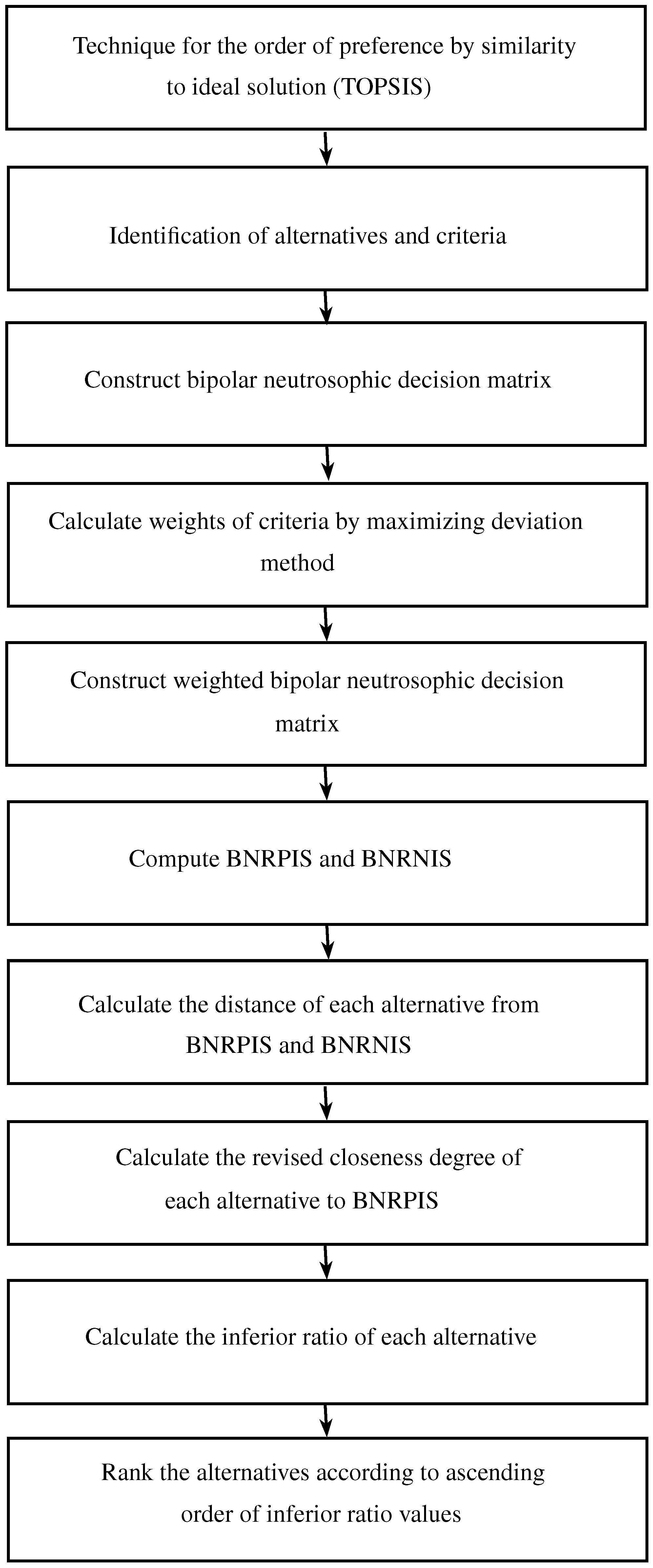
2. Bipolar Neutrosophic TOPSIS Method

Definition 1.

Ref. [4] Let C be a nonempty set. A bipolar neutrosophic set (BNS) $\tilde{B}$ on C is defined as follows

$$\begin{array}{c}\hfill \tilde{B}=\{c,〈T_{\tilde{B}}^{+}\left(c\right),I_{\tilde{B}}^{+}\left(c\right),F_{\tilde{B}}^{+}\left(c\right),T_{\tilde{B}}^{-}\left(c\right),I_{\tilde{B}}^{-}\left(c\right),F_{\tilde{B}}^{-}\left(c\right)〉|c\in C\},\end{array}$$

where, $T_{\tilde{B}}^{+}\left(c\right),I_{\tilde{B}}^{+}\left(c\right),F_{\tilde{B}}^{+}\left(c\right):C\to [0,1]and{T}_{\tilde{B}}^{-}\left(c\right),I_{\tilde{B}}^{-}\left(c\right),F_{\tilde{B}}^{-}\left(c\right):C\to [-1,0]$.

We now describe our proposed bipolar neutrosophic TOPSIS method.

Let $S=\{S_1,S_2,\cdots ,S_m\}$ be a set of m favorable alternatives and let $T=\{T_1,T_2,\cdots ,T_n\}$ be a set of n attributes. Let $W={[w_1{w}_2\cdots w_n]}^T$ be the weight vector such that $0\le w_j\le 1$ and ${\displaystyle \sum _{j=1}^n}{w}_j=1.$ Suppose that the rating value of each alternative $S_i,(i=1,2,\cdots ,m)$ with respect to the attributes $T_j,(j=1,2,\cdots ,n)$ is given by decision maker in the form of bipolar neutrosophic sets (BNSs). The steps of bipolar neutrosophic TOPSIS method are described as follows:

(i)

Each value of alternative is estimated with respect to n criteria. The value of each alternative under each criterion is given in the form of BNSs and they can be expressed in the decision matrix as

$$K={\left[k_{ij}\right]}_{m\times n}=\left[\begin{array}{cccc}{k}_{11}& k_{12}& \cdots & k_{1n}\\ k_{21}& k_{22}& \cdots & k_{2n}\\ ·& ·& \cdots & .\\ ·& ·& \cdots & ·\\ k_{m1}& k_{m2}& \cdots & k_{mn}\end{array}\right].$$

Each entry $k_{ij}=<T_{ij}^{+},I_{ij}^{+},F_{ij}^{+},T_{ij}^{-},I_{ij}^{-},F_{ij}^{-}>$, where, $T_{ij}^{+},I_{ij}^{+}$ and $F_{ij}^{+}$ represent the degree of positive truth, indeterminacy and falsity membership, respectively, whereas, $T_{ij}^{-},I_{ij}^{-}$ and $F_{ij}^{-}$ represent the degree of negative truth, indeterminacy and falsity membership, respectively, such that $T_{ij}^{+},I_{ij}^{+},F_{ij}^{+}\in [0,1]$, $T_{ij}^{-},I_{ij}^{-},F_{ij}^{-}\in [-1,0]$ and $0\le T_{ij}^{+}+I_{ij}^{+}+F_{ij}^{+}-T_{ij}^{-}-I_{ij}^{-}-F_{ij}^{-}\le 6$, $i=1,2,3,\dots ,m$; $j=1,2,3,\dots ,n$.

(ii)

Suppose that the weights of the criteria are not equally assigned and they are totally unknown to the decision maker. We use the maximizing deviation method [30] to determine the unknown weights of the criteria. Therefore, the weight of the attribute $T_j$ is given as

$$\begin{array}{c}\hfill w_j=\frac{{\displaystyle \sum _{i=1}^m}{\displaystyle \sum _{l=1}^m}|k_{ij}-k_{lj}|}{\sqrt{{\displaystyle \sum _{j=1}^n}{\left({\displaystyle \sum _{i=1}^m}{\displaystyle \sum _{l=1}^m}|k_{ij}-k_{lj}|\right)}^2}},\end{array}$$

and the normalized weight of the attribute $T_j$ is given as

$$\begin{array}{c}\hfill w_j^{*}=\frac{{\displaystyle \sum _{i=1}^m}{\displaystyle \sum _{l=1}^m}|k_{ij}-k_{lj}|}{{\displaystyle \sum _{j=1}^n}\left({\displaystyle \sum _{i=1}^m}{\displaystyle \sum _{l=1}^m}|k_{ij}-k_{lj}|\right)}.\end{array}$$

(iii)

The accumulated weighted bipolar neutrosophic decision matrix is computed by multiplying the weights of the attributes to aggregated decision matrix as follows:

$$K\otimes W={\left[k_{ij}^{w_j}\right]}_{m\times n}=\left[\begin{array}{cccc}{k}_{11}^{w_1}& k_{12}^{w_2}& \cdots & k_{1n}^{w_n}\\ k_{21}^{w_1}& k_{22}^{w_2}& \cdots & k_{2n}^{w_n}\\ ·& ·& \cdots & ·\\ ·& ·& \cdots & ·\\ k_{m1}^{w_1}& k_{m2}^{w_2}& \cdots & k_{mn}^{w_n}\end{array}\right].$$

where

$$\begin{array}{cc}\hfill k_{ij}^{w_j}& =<T_{ij}^{w_j+},I_{ij}^{w_j+},F_{ij}^{w_j+},T_{ij}^{w_j-},I_{ij}^{w_j-},F_{ij}^{w_j-}>\hfill \\ & =<1-{(1-T_{ij}^{+})}^{w_j},{(I_{ij}^{+})}^{w_j},{(F_{ij}^{+})}^{w_j},-{(-T_{ij}^{-})}^{w_j},-{(-I_{ij}^{-})}^{w_j},-(1-{(1-(-F_{ij}^{-}))}^{w_j})>,\hfill \end{array}$$

(iv)

Two types of attributes, benefit type attributes and cost type attributes, are mostly applicable in real life decision making. The bipolar neutrosophic relative positive ideal solution (BNRPIS) and bipolar neutrosophic relative negative ideal solution (BNRNIS) for both type of attributes are defined as follows:

$$\begin{array}{ccc}\hfill BNRPIS& =& (〈{}^{+}{T}_1^{w_1+}{,}^{+}{I}_1^{w_1+}{,}^{+}{F}_1^{w_1+}{,}^{+}{T}_1^{w_1-}{,}^{+}{I}_1^{w_1-}{,}^{+}{F}_1^{w_1-}〉,{\langle }^{+}{T}_2^{w_2+}{,}^{+}{I}_2^{w_2+}{,}^{+}{F}_2^{w_2+}{,}^{+}{T}_2^{w_2-},\hfill \\ & & \hfill {}^{+}{I}_2^{w_2-}{,}^{+}{F}_2^{w_2-}\rangle ,\dots ,〈{}^{+}{T}_n^{w_n+}{,}^{+}{I}_n^{w_n+}{,}^{+}{F}_n^{w_n+}{,}^{+}{T}_n^{w_n-}{,}^{+}{I}_n^{w_n-}{,}^{+}{F}_n^{w_n-}〉),\\ \hfill BNRNIS& =& (〈{}^{-}{T}_1^{w_1+}{,}^{-}{I}_1^{w_1+}{,}^{-}{F}_1^{w_1+}{,}^{-}{T}_1^{w_1-}{,}^{-}{I}_1^{w_1-}{,}^{-}{F}_1^{w_1-}〉,{\langle }^{-}{T}_2^{w_2+}{,}^{-}{I}_2^{w_2+}{,}^{-}{F}_2^{w_2+}{,}^{-}{T}_2^{w_2-},\hfill \\ & & \hfill {}^{-}{I}_2^{w_2-}{,}^{-}{F}_2^{w_2-}\rangle ,...,〈{}^{-}{T}_n^{w_n+}{,}^{-}{I}_n^{w_n+}{,}^{-}{F}_n^{w_n+}{,}^{-}{T}_n^{w_n-}{,}^{-}{I}_n^{w_n-}{,}^{-}{F}_n^{w_n-}〉),\end{array}$$

such that, for benefit type criteria, $j=1,2,\dots ,n$

$$\begin{array}{ccc}\hfill 〈{}^{+}{T}_j^{w_j+}{,}^{+}{I}_j^{w_j+}{,}^{+}{F}_j^{w_j+}{,}^{+}{T}_j^{w_j-}{,}^{+}{I}_j^{w_j-}{,}^{+}{F}_j^{w_j-}〉& =& \langle max\left(T_{ij}^{w_j+}\right),min\left(I_{ij}^{w_j+}\right),min\left(F_{ij}^{w_j+}\right),\hfill \\ & & min\left(T_{ij}^{w_j-}\right),max\left(I_{ij}^{w_j-}\right),max\left(F_{ij}^{w_j-}\right)\rangle ,\hfill \\ \hfill 〈{}^{-}{T}_j^{w_j+}{,}^{-}{I}_j^{w_j+}{,}^{-}{F}_j^{w_j+}{,}^{-}{T}_j^{w_j-}{,}^{-}{I}_j^{w_j-}{,}^{-}{F}_j^{w_j-}〉& =& \langle min\left(T_{ij}^{w_j+}\right),max\left(I_{ij}^{w_j+}\right),max\left(F_{ij}^{w_j+}\right),\hfill \\ & & max\left(T_{ij}^{w_j-}\right),min\left(I_{ij}^{w_j-}\right),min\left(F_{ij}^{w_j-}\right)\rangle .\hfill \end{array}$$

Similarly, for cost type criteria, $j=1,2,\dots ,n$

$$\begin{array}{ccc}\hfill 〈{}^{+}{T}_j^{w_j+}{,}^{+}{I}_j^{w_j+}{,}^{+}{F}_j^{w_j+}{,}^{+}{T}_j^{w_j-}{,}^{+}{I}_j^{w_j-}{,}^{+}{F}_j^{w_j-}〉& =& \langle min\left(T_{ij}^{w_j+}\right),max\left(I_{ij}^{w_j+}\right),max\left(F_{ij}^{w_j+}\right),\hfill \\ & & max\left(T_{ij}^{w_j-}\right),min\left(I_{ij}^{w_j-}\right),min\left(F_{ij}^{w_j-}\right)\rangle ,\hfill \\ \hfill 〈{}^{-}{T}_j^{w_j+}{,}^{-}{I}_j^{w_j+}{,}^{-}{F}_j^{w_j+}{,}^{-}{T}_j^{w_j-}{,}^{-}{I}_j^{w_j-}{,}^{-}{F}_j^{w_j-}〉& =& \langle max\left(T_{ij}^{w_j+}\right),min\left(I_{ij}^{w_j+}\right),min\left(F_{ij}^{w_j+}\right),\hfill \\ & & min\left(T_{ij}^{w_j-}\right),max\left(I_{ij}^{w_j-}\right),max\left(F_{ij}^{w_j-}\right)\rangle .\hfill \end{array}$$

(v)

The normalized Euclidean distance of each alternative $〈T_{ij}^{w_j+},I_{ij}^{w_j+},F_{ij}^{w_j+},T_{ij}^{w_j-},I_{ij}^{w_j-},F_{ij}^{w_j-}〉$ from the BNRPIS $〈{}^{+}{T}_j^{w_j+}{,}^{+}{I}_j^{w_j+}{,}^{+}{F}_j^{w_j+}{,}^{+}{T}_j^{w_j-}{,}^{+}{I}_j^{w_j-}{,}^{+}{F}_j^{w_j-}〉$ can be calculated as

$$d_N(S_i,BNRPIS)=\sqrt{\frac{1}{6n}{\displaystyle \sum _{j=1}^n}\left\{\begin{array}{c}{\left(T_{ij}^{w_j+}{-}^{+}{T}_j^{w_j+}\right)}^2+{\left(I_{ij}^{w_j+}{-}^{+}{I}_j^{w_j+}\right)}^2+{\left(F_{ij}^{w_j+}{-}^{+}{F}_j^{w_j+}\right)}^2+\hfill \\ \hfill {\left(T_{ij}^{w_j-}{-}^{+}{T}_j^{w_j-}\right)}^2+{\left(I_{ij}^{w_j-}{-}^{+}{I}_j^{w_j-}\right)}^2+{\left(F_{ij}^{w_j-}{-}^{+}{F}_j^{w_j-}\right)}^2\end{array}\right\}},$$

and the normalized Euclidean distance of each alternative $〈T_{ij}^{w_j+},I_{ij}^{w_j+},F_{ij}^{w_j+},T_{ij}^{w_j-},I_{ij}^{w_j-},F_{ij}^{w_j-}〉$ from the BNRNIS $〈{}^{-}{T}_j^{w_j+}{,}^{-}{I}_j^{w_j+}{,}^{-}{F}_j^{w_j+}{,}^{-}{T}_j^{w_j-}{,}^{-}{I}_j^{w_j-}{,}^{-}{F}_j^{w_j-}〉$ can be calculated as

$$d_N(S_i,BNRNIS)=\sqrt{\frac{1}{6n}\underset{j=1}{\sum ^n}\left\{\begin{array}{c}{\left(T_{ij}^{w_j+}{-}^{-}{T}_j^{w_j+}\right)}^2+{\left(I_{ij}^{w_j+}{-}^{-}{I}_j^{w_j+}\right)}^2+{\left(F_{ij}^{w_j+}{-}^{-}{F}_j^{w_j+}\right)}^2+\hfill \\ \hfill {\left(T_{ij}^{w_j-}{-}^{-}{T}_j^{w_j-}\right)}^2+{\left(I_{ij}^{w_j-}{-}^{-}{I}_j^{w_j-}\right)}^2+{\left(F_{ij}^{w_j-}{-}^{-}{F}_j^{w_j-}\right)}^2\end{array}\right\}}.$$

(vi)

Revised closeness degree of each alternative to BNRPIS represented as ${\rho }_i$ and it is calculated using formula

$$\begin{array}{c}\hfill \rho \left(S_i\right)=\frac{d_N(S_i,BNRNIS)}{max\left\{d_N(S_i,BNRNIS)\right\}}-\frac{d_N(S_i,BNRPIS)}{min\left\{d_N(S_i,BNRPIS)\right\}},i=1,2,\dots ,m.\end{array}$$

(vii)

By using the revised closeness degrees, the inferior ratio to each alternative is determined as follows:

$$\begin{array}{c}\hfill IR\left(i\right)=\frac{\rho \left(S_i\right)}{\underset{1\le i\le m}{min}\left(\rho \left(S_i\right)\right)}.\end{array}$$

It is clear that each value of $IR\left(i\right)$ lies in the closed unit interval [0,1].

(viii)

The alternatives are ranked according to the ascending order of inferior ratio values and the best alternative with minimum choice value is chosen.

Geometric representation of the procedure of our proposed bipolar neutrosophic TOPSIS method is shown in Figure 1.

3. Applications

In this section, we apply bipolar neutrosophic TOPSIS method to solve real life problems: the best electronic commerce web site, heart surgeon and employee were chosen.

3.1. Electronic Commerce Web Site

Electronic Commerce (e-commerce, for short) is a process of trading the services and goods through electronic networks like computer structures as well as the internet. In recent times e-commerce has become a very fascinating and convenient choice for both the businesses and customers. Many companies are interested in advancing their online stores rather than the brick and mortar buildings, because of the appealing requirements of customers for online purchasing. Suppose that a person wants to launch his own online store for selling his products. He will choose the e-commerce web site that has comparatively better ratings and that is most popular among internet users. After initial screening four web sites, $S_1=$ Shopify, $S_2=3d$ Cart, $S_3=$ BigCommerce and $S_4=$ Shopsite, are considered. Four attributes, $T_1=$ Customer satisfaction, $T_2=$ Comparative prices, $T_3=$ On-time delivery and $T_4=$ Digital marketing, are designed to choose the best alternative.

Step 1.

The decision matrix in the form of bipolar neutrosophic information is given as in

Table 1. Bipolar neutrosophic decision matrix.

$\mathit{S}\setminus \mathit{T}$	${\mathit{T}}_1$	${\mathit{T}}_2$	${\mathit{T}}_3$	${\mathit{T}}_4$
$S_1$	($0.4,0.2,0.5,$	($0.5,0.3,0.3,$	($0.2,0.7,0.5,$	($0.4,0.6,0.5,$
	$-0.6,-0.4,-0.4$)	$-0.7,-0.2,-0.4$)	$-0.4,-0.4,-0.3$)	$-0.3,-0.7,-0.4$)
$S_2$	($0.3,0.6,0.1,$	($0.2,0.6,0.1,$	($0.4,0.2,0.5,$	($0.2,0.7,0.5,$
	$-0.5,-0.7,-0.5$)	$-0.5,-0.3,-0.7$)	$-0.6,-0.3,-0.1$)	$-0.5,-0.3,-0.2$)
$S_3$	($0.3,0.5,0.2,$	($0.4,0.5,0.2,$	($0.9,0.5,0.7,$	($0.3,0.7,0.6,$
	$-0.4,-0.3,-0.7$)	$-0.3,-0.8,-0.5$)	$-0.3,-0.4,-0.3$)	$-0.5,-0.5,-0.4$)
$S_4$	($0.6,0.7,0.5,$	($0.8,0.4,0.6,$	($0.6,0.3,0.6,$	($0.8,0.3,0.2,$
	$-0.2,-0.1,-0.3$)	$-0.1,-0.3,-0.4$)	$-0.1,-0.4,-0.2$)	$-0.1,-0.3,-0.1$)

:

Step 2.

The normalized weights of the criteria are calculated by using maximizing deviation method as given below:

$$w_1=0.2567,w_2=0.2776,w_3=0.2179,w_4=0.2478,\mathrm{where}{\displaystyle \sum _{j=1}^4}{w}_j=1.$$

Step 3.

The weighted bipolar neutrosophic decision matrix is constructed by multiplying the weights to decision matrix as given in

Table 2. Weighted bipolar neutrosophic decision matrix.

$\mathit{S}\setminus \mathit{T}$	${\mathit{T}}_1$	${\mathit{T}}_2$	${\mathit{T}}_3$	${\mathit{T}}_4$
$S_1$	$(0.123,0.662,0.837,$	$(0.175,0.716,0.716,$	$(0.047,0.925,0.86,$	$(0.119,0.881,0.842,$
	$-0.877,-0.79,-0.123)$	$-0.906,-0.64,-0.132)$	$-0.819,-0.819,-0.075)$	$-0.742,-0.915,-0.119)$
$S_2$	$(0.087,0.877,0.554,$	$(0.06,0.868,0.528,$	$(0.105,0.704,0.86,$	$(0.054,0.915,0.842,$
	$-0.837,-0.913,-0.163)$	$-0.825,-0.716,-0.284)$	$-0.895,-0.769,-0.023)$	$-0.842,-0.742,-0.054)$
$S_3$	$(0.087,0.837,0.662,$	$(0.132,0.825,0.64,$	$(0.395,0.86,0.925,$	$(0.085,0.915,0.881,$
	$-0.79,-0.734,-0.226)$	$-0.716,-0.94,-0.175)$	$-0.769,-0.819,-0.75)$	$-0.842,-0.842,-0.119)$
$S_4$	$(0.21,0.913,0.837,$	$(0.36,0.775,0.868,$	$(0.181,0.769,0.895,$	$(0.329,0.742,0.671,$
	$-0.662,-0.554,-0.087)$	$-0.528,-0.716,-0.132)$	$-0.605,-0.819,-0.047)$	$-0.565,-0.742,-0.026)$

:

Step 4.

The BNRPIS and BNRNIS are given by

$$\begin{array}{ccc}\hfill BNRPIS& =& \hfill <(0.21,0.662,0.554,-0.877,-0.554,-0.087),\\ & & \hfill (0.06,0.868,0.868,-0.528,-0.94,-0.284),\\ & & \hfill (0.395,0.704,0.86,-0.895,-0.769,-0.023),\\ & & \hfill (0.329,0.742,0.671,-0.842,-0.742,-0.062)>;\end{array}$$

$$\begin{array}{ccc}\hfill BNRNIS& =& \hfill <(0.087,0.913,0.837,-0.662,-0.913,-0.266),\\ & & \hfill (0.36,0.716,0.528,-0.906,-0.64,-0.132),\\ & & \hfill (0.047,0.925,0.925,-0.605,-0.819,-0.075),\\ & & \hfill (0.054,0.915,0.881,-0.565,-0.915,-0.119)>.\end{array}$$

Step 5.

The normalized Euclidean distances of each alternative from the BNRPISs and the BNRNISs are given as follows:

$$\begin{array}{cc}\hfill d_N(S_1,BNRPIS)& =0.1805,d_N(S_1,BNRNIS)=0.1125,\hfill \\ \hfill d_N(S_2,BNRPIS)& =0.1672,d_N(S_2,BNRNIS)=0.1485,\hfill \\ \hfill d_N(S_3,BNRPIS)& =0.135,d_N(S_3,BNRNIS)=0.1478,\hfill \\ \hfill d_N(S_4,BNRPIS)& =0.155,d_N(S_4,BNRNIS)=0.1678.\hfill \end{array}$$

Step 6.

The revised closeness degree of each alternative is given as

$$\rho \left(S_1\right)=-0.667,\rho \left(S_2\right)=-0.334,\rho \left(S_3\right)=-0.119,\rho \left(S_4\right)=-0.148.$$

Step 7.

The inferior ratio to each alternative is given as

$$IR\left(1\right)=1,IR\left(2\right)=0.52,IR\left(3\right)=0.18,IR\left(4\right)=0.22.$$

Step 8.

Ordering the web stores according to ascending order of alternatives, we obtain: $S_3<S_4<S_2<S_1$. Therefore, the person will choose the BigCommerce for opening a web store.

3.2. Heart Surgeon

Suppose that a heart patient wants to select a best cardiac surgeon for heart surgery. After initial screening, five surgeons are considered for further evaluation. These surgeons represent the alternatives and are denoted by $S_1,S_2,S_3,S_4$, and $S_5$ in our MCDM problem. Suppose that he concentrates on four characteristics, $T_1=$ Availability of medical equipment, $T_2=$ Surgeon reputation, $T_3=$ Expenditure and $T_4=$ Suitability of time, in order to select the best surgeon. These characteristics represent the criteria for this MCDM problem.

Step 1.

The decision matrix in the form of bipolar neutrosophic information is given as in

Table 3. Bipolar neutrosophic decision matrix.

$\mathit{S}\setminus \mathit{T}$	${\mathit{T}}_1$	${\mathit{T}}_2$	${\mathit{T}}_3$	${\mathit{T}}_4$
$S_1$	$(0.6,0.5,0.3,$	$(0.5,0.7,0.4,$	$(0.3,0.5,0.5,$	$(0.5,0.3,0.6,$
	$-0.5,-0.7,-0.4)$	$-0.6,-0.4,-0.5)$	$-0.7,-0.3,-0.4)$	$-0.4,-0.7,-0.5)$
$S_2$	$(0.9,0.3,0.2,$	$(0.7,0.4,0.2,$	$(0.4,0.7,0.6,$	$(0.8,0.3,0.2,$
	$-0.3,-0.6,-0.5)$	$-0.4,-0.5,-0.7)$	$-0.6,-0.3,-0.3)$	$-0.5,-0.5,-0.7)$
$S_3$	$(0.4,0.6,0.6,$	$(0.5,0.3,0.6,$	$(0.7,0.5,0.3,$	$(0.4,0.6,0.7,$
	$-0.7,-0.4,-0.3)$	$-0.6,-0.4,-0.4)$	$-0.4,-0.4,-0.6)$	$-0.5,-0.4,-0.4)$
$S_4$	$(0.8,0.5,0.3,$	$(0.6,0.4,0.3,$	$(0.4,0.5,0.7,$	$(0.5,0.4,0.6,$
	$-0.3,-0.4,-0.5)$	$-0.5,-0.7,-0.8)$	$-0.5,-0.4,-0.2)$	$-0.6,-0.7,-0.3)$
$S_5$	$(0.6,0.4,0.6,$	$(0.4,0.7,0.6,$	$(0.6,0.3,0.5,$	$(0.5,0.7,0.4$,
	$-0.4,-0.7,-0.3)$	$-0.7,-0.5,-0.6)$	$-0.3,-0.7,-0.4)$	$-0.3,-0.6,-0.5)$

:

Step 2.

The normalized weights of the criteria are calculated by using maximizing deviation method as given below:

$$w_1=0.2480,w_2=0.2424,w_3=0.2480,w_4=0.2616,\mathrm{where}{\displaystyle \sum _{j=1}^4}{w}_j=1.$$

Step 3.

The weighted bipolar neutrosophic decision matrix is constructed by multiplying the weights to decision matrix as given in

Table 4. Weighted bipolar neutrosophic decision matrix.

$\mathit{S}\setminus \mathit{T}$	${\mathit{T}}_1$	${\mathit{T}}_2$	${\mathit{T}}_3$	${\mathit{T}}_4$
$S_1$	$(0.203,0.842,0.742,$	$(0.155,0.917,0.801,$	$(0.085,0.842,0.842,$	$(0.166,0.730,0.875,$
	$-0.842,-0.915,-0.119)$	$-0.884,-0.801,-0.677)$	$-0.915,-0.742,-0.119)$	$-0.787,-0.911,-0.166)$
$S_2$	$(0.435,0.742,0.671,$	$(0.253,0.801,0.677,$	$(0.119,0.915,0.881,$	$(0.344,0.730,0.656,$
	$-0.742,-0.881,-0.158)$	$-0.801,-0.845,-0.253)$	$-0.881,-0.742,-0.085)$	$-0.656,-0.834,-0.270)$
$S_3$	$(0.119,0.881,0.881,$	$(0.155,0.747,0.884,$	$(0.258,0.842,0.742,$	$(0.125,0.875,0.911,$
	$-0.915,-0.797,-0.085)$	$-0.884,-0.801,-0.116)$	$-0.797,-0.797,-0.203)$	$-0.834,-0.787,-0.125)$
$S_4$	$(0.329,0.842,0.742,$	$(0.199,0.801,0.747,$	$(0.119,0.842,0.915,$	$(0.166,0.787,0.875,$
	$-0.742,-0.797,-0.158)$	$-0.845,-0.917,-0.323)$	$-0.842,-0.797,-0.054)$	$-0.875,-0.911,-0.089)$
$S_5$	$(0.203,0.797,0.881,$	$(0.116,0.917,0.884,$	$(0.203,0.742,0.842,$	$(0.166,0.911,0.787,$
	$-0.797,-0.915,-0.085)$	$-0.917,-0.845,-0.199)$	$-0.742,-0.915,-0.119)$	$-0.730,-0.875,-0.166)$

:

Step 4.

The BNRPIS and BNRNIS are given by

$$\begin{array}{ccc}\hfill BNRPIS& =& \hfill <(0.435,0.742,0.671,-0.915,-0.797,-0.085),\\ & & \hfill (0.253,0.747,0.677,-0.917,-0.801,-0.116),\\ & & \hfill (0.085,0.915,0.915,-0.742,-0.915,-0.203),\\ & & \hfill (0.344,0.730,0.656,-0.875,-0.787,-0.089)>;\end{array}$$

$$\begin{array}{ccc}\hfill BNRNIS& =& \hfill <(0.119,0.881,0.881,-0.742,-0.915,-0.158),\\ & & \hfill (0.116,0.917,0.884,-0.801,-0.917,-0.323),\\ & & \hfill (0.258,0.742,0.742,-0.915,-0.742,-0.054),\\ & & \hfill (0.125,0.911,0.911,-0.656,-0.911,-0.270)>.\end{array}$$

Step 5.

The normalized Euclidean distances of each alternative from the BNRPISs and the BNRNISs are given as follows:

$$\begin{array}{cc}\hfill d_N(S_1,BNRPIS)& =0.1176,d_N(S_1,BNRNIS)=0.0945,\hfill \\ \hfill d_N(S_2,BNRPIS)& =0.0974,d_N(S_2,BNRNIS)=0.1402,\hfill \\ \hfill d_N(S_3,BNRPIS)& =0.1348,d_N(S_3,BNRNIS)=0.1043,\hfill \\ \hfill d_N(S_4,BNRPIS)& =0.1089,d_N(S_4,BNRNIS)=0.1093,\hfill \\ \hfill d_N(S_5,BNRPIS)& =0.1292,d_N(S_5,BNRNIS)=0.0837.\hfill \end{array}$$

Step 6.

The revised closeness degree of each alternative is given as

$$\rho \left(S_1\right)=-0.553,\rho \left(S_2\right)=0,\rho \left(S_3\right)=-0.64,\rho \left(S_4\right)=-0.338,\rho \left(S_5\right)=-0.729$$

Step 7.

The inferior ratio to each alternative is given as

$$IR\left(1\right)=0.73,IR\left(2\right)=0,IR\left(3\right)=0.88,IR\left(4\right)=0.46,IR\left(5\right)=1.$$

Step 8.

Ordering the alternatives in ascending order, we obtain: $S_2<S_4<S_1<S_3<S_5$. Therefore, $S_2$ is best among all other alternatives.

3.3. Employee (Marketing Manager)

Process of employee selection has an analytical importance for any kind of business. According to firm hiring requirements and the job position, this process may vary from a very simple process to a complicated procedure. Suppose that a company wants to hire an employee for the post of marketing manager. After initial screening, four candidates are considered as alternatives and denoted by $S_1,S_2,S_3\mathrm{and}{S}_4$ in our MCDM problem. The requirements for this post, $T_1=$ Confidence, $T_2=$ Qualification, $T_3=$ Leading skills and $T_4=$ Communication skills, are considered as criteria in order to select the most relevant candidate.

Step 1.

The decision matrix in the form of bipolar neutrosophic information is given as in

Table 5. Bipolar neutrosophic decision matrix.

$\mathit{S}\setminus \mathit{T}$	${\mathit{T}}_1$	${\mathit{T}}_2$	${\mathit{T}}_3$	${\mathit{T}}_4$
$S_1$	$(0.8,0.5,0.3,$	$(0.7,0.3,0.2,$	$(0.5,0.4,0.6,$	$(0.9,0.3,0.2,$
	$-0.3,-0.6,-0.5)$	$-0.3,-0.5,-0.4)$	$-0.5,-0.3,-0.4)$	$-0.3,-0.4,-0.2)$
$S_2$	$(0.5,0.7,0.6$	$(0.4,0.7,0.5,$	$(0.6,0.8,0.5,$	$(0.5,0.3,0.6,$
	$-0.4,-0.2,-0.4)$	$-0.6,-0.2,-0.3)$	$-0.3,-0.5,-0.7)$	$-0.6,-0.4,-0.3)$
$S_3$	$(0.4,0.6,0.8,$	$(0.6,0.3,0.5,$	$(0.3,0.5,0.7,$	$(0.5,0.7,0.4,$
	$-0.7,-0.3,-0.4)$	$-0.2,-0.4,-0.6)$	$-0.8,-0.4,-0.2)$	$-0.6,-0.3,-0.5)$
$S_4$	$(0.7,0.3,0.5,$	$(0.5,0.4,0.6,$	$(0.6,0.4,0.3,$	$(0.4,0.5,0.7,$
	$-0.4,-0.2,-0.5)$	$-0.4,-0.5,-0.3)$	$-0.3,-0.5,-0.7)$	$-0.6,-0.5,-0.3)$

:

Step 2.

The normalized weights of the criteria are calculated by using maximizing deviation method as given below:

$$w_1=0.25,w_2=0.2361,w_3=0.2708,w_4=0.2431,\mathrm{where}{\displaystyle \sum _{j=1}^4}{w}_j=1.$$

Step 3.

The weighted bipolar neutrosophic decision matrix is constructed by multiplying the weights to decision matrix as given in

Table 6. Weighted bipolar neutrosophic decision matrix.

$\mathit{S}\setminus \mathit{T}$	${\mathit{T}}_1$	${\mathit{T}}_2$	${\mathit{T}}_3$	${\mathit{T}}_4$
$S_1$	$(0.3313,0.8409,0.7401,$	$(0.2474,0.7526,0.6839,$	$(0.1711,0.7803,0.8708,$	$(0.4287,0.7463,0.6762,$
	$-0.7401,-0.8801,-0.1591)$	$-0.7256,-0.8490,-0.1136)$	$-0.8289,-0.7218,-0.1292)$	$-0.7463,-0.8003,-0.0528)$
$S_2$	$(0.1591,0.9147,0.8801,$	$(0.1136,0.9192,0.8490,$	$(0.2197,0.9414,0.8289,$	$(0.1551,0.7463,0.8832,$
	$-0.7953,-0.6687,-0.1199)$	$-0.8864,-0.6839,-0.0808)$	$-0.7218,-0.8289,-0.2782)$	$-0.8832,-0.8003,-0.0831)$
$S_3$	$(0.1199,0.8801,0.9457,$	$(0.1945,0.7526,0.8490,$	$(0.0921,0.8289,0.9079,$	$(0.1551,0.9169,0.8003,$
	$-0.9147,-0.7401,-0.1199)$	$-0.6839,-0.8055,-0.1945)$	$-0.9414,-0.7803,-0.0586)$	$-0.8832,-0.7463,-0.1551)$
$S_4$	$(0.2599,0.7401,0.8409,$	$(0.1510,0.8055,0.8864,$	$(0.2197,0.7803,0.7218,$	$(0.1168,0.8449,0.9169,$
	$-0.7953,-0.6687,-0.1591)$	$-0.8055,-0.8490,-0.0808)$	$-0.7218,-0.8289,-0.2782)$	$-0.8832,-0.8449,-0.0831)$

:

Step 4.

The BNRPIS and BNRNIS are given by

$$\begin{array}{ccc}\hfill BNRPIS& =& \hfill <(0.3313,0.7401,0.7401,-0.9147,-0.6687,-0.1199),\\ & & \hfill (0.2474,0.7526,0.6839,-0.8864,-0.6839,-0.0808),\\ & & \hfill (0.2197,0.7803,0.7218,-0.9414,-0.7218,-0.0586),\\ & & \hfill (0.4287,0.7463,0.6762,-0.8832,-0.7463,-0.0528)>;\end{array}$$

$$\begin{array}{ccc}\hfill BNRNIS& =& \hfill <(0.1199,0.9147,0.9457,-0.7401,-0.8801,-0.1591),\\ & & \hfill (0.1136,0.9192,0.8864,-0.6839,-0.8490,-0.1945),\\ & & \hfill (0.0921,0.9414,0.9079,-0.7218,-0.8289,-0.2782),\\ & & \hfill (0.1168,0.9169,0.9169,-0.7463,-0.8449,-0.1551)>.\end{array}$$

Step 5.

The normalized Euclidean distances of each alternative from the BNRPISs and the BNRNISs are given as follows:

$$\begin{array}{cc}\hfill d_N(S_1,BNRPIS)& =0.0906,d_N(S_1,BNRNIS)=0.1393,\hfill \\ \hfill d_N(S_2,BNRPIS)& =0.1344,d_N(S_2,BNRNIS)=0.0953,\hfill \\ \hfill d_N(S_3,BNRPIS)& =0.1286,d_N(S_3,BNRNIS)=0.1011,\hfill \\ \hfill d_N(S_4,BNRPIS)& =0.1293,d_N(S_4,BNRNIS)=0.0999.\hfill \end{array}$$

Step 6.

The revised closeness degree of each alternative is given as

$$\rho \left(S_1\right)=0,\rho \left(S_2\right)=-0.799,\rho \left(S_3\right)=-0.694,\rho \left(S_4\right)=-0.780.$$

Step 7.

The inferior ratio to each alternative is given as

$$IR\left(1\right)=0,IR\left(2\right)=1,IR\left(3\right)=0.87,IR\left(4\right)=0.98.$$

Step 8.

Ordering the alternatives in ascending order, we obtain: $S_1<S_3<S_4<S_2$. Therefore, the company will select the candidate $S_1$ for this post.

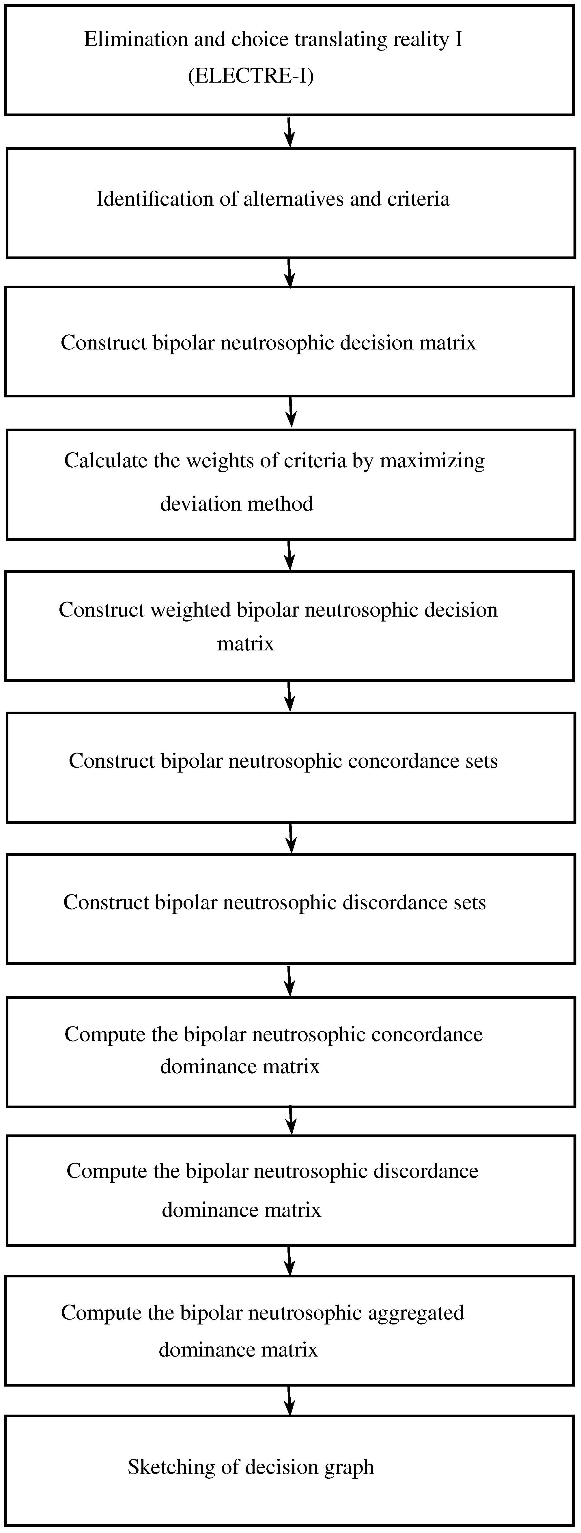
4. Bipolar Neutrosophic ELECTRE-I Method

In this section, we propose bipolar neutrosophic ELECTRE-I method to solve MCDM problems. Consider a set of alternatives, denoted by $S=\{S_1,S_2,S_3,\cdots ,S_m\}$ and the set of criteria, denoted by $T=\{T_1,T_2,T_3,\cdots ,T_n\}$ which are used to evaluate the alternatives.

(i–iii)

As in the section of bipolar neutrosophic TOPSIS, the rating values of alternatives with respect to the criteria are expressed in the form of matrix ${\left[k_{ij}\right]}_{m\times n}$. The weights $w_j$ of the criteria $T_j$ are evaluated by maximizing deviation method and the weighted bipolar neutrosophic decision matrix ${\left[k_{ij}^{w_j}\right]}_{m\times n}$ is constructed.

(iv)

The bipolar neutrosophic concordance sets $E_{xy}$ and bipolar neutrosophic discordance sets $F_{xy}$ are defined as follows:

$$\begin{array}{c}\hfill E_{xy}=\{1\le j\le n|{\rho }_{xj}\ge {\rho }_{yj}\},x\ne y,x,y=1,2,\cdots ,m,\\ \hfill F_{xy}=\{1\le j\le n|{\rho }_{xj}\le {\rho }_{yj}\},x\ne y,x,y=1,2,\cdots ,m,\end{array}$$

where, ${\rho }_{ij}=T_{ij}^{+}+I_{ij}^{+}+F_{ij}^{+}+T_{ij}^{-}+I_{ij}^{-}+F_{ij}^{-},i=1,2,\cdots ,m,j=1,2,\cdots ,n$.

(v)

The bipolar neutrosophic concordance matrix E is constructed as follows:

$$E=\left[\begin{array}{cccccc}-& e_{12}& ·& ·& ·& e_{1m}\\ e_{21}& -& ·& ·& ·& e_{2m}\\ ·\\ ·\\ ·\\ e_{m1}& e_{m2}& ·& ·& ·& -\end{array}\right],$$

where, the bipolar neutrosophic concordance indices $e_{{xy}^{\prime }}s$ are determined as

$$\begin{array}{c}\hfill e_{xy}=\sum _{j\in E_{xy}}{w}_j.\end{array}$$

(vi)

The bipolar neutrosophic discordance matrix F is constructed as follows:

$$F=\left[\begin{array}{cccccc}-& f_{12}& ·& ·& ·& f_{1m}\\ f_{21}& -& ·& ·& ·& f_{2m}\\ ·\\ ·\\ ·\\ f_{m1}& f_{m2}& ·& ·& ·& -\end{array}\right],$$

where, the bipolar neutrosophic discordance indices $f_{{xy}^{\prime }}s$ are determined as

$$\begin{array}{c}\hfill f_{xy}=\frac{\underset{j\in F_{xy}}{max}\sqrt{\frac{1}{6n}\left\{\begin{array}{c}{(T_{xj}^{w_j+}-T_{yj}^{w_j+})}^2+{(I_{xj}^{w_j+}-I_{yj}^{w_j+})}^2+{(F_{xj}^{w_j+}-F_{yj}^{w_j+})}^2+\hfill \\ \hfill {(T_{xj}^{w_j-}-T_{yj}^{w_j-})}^2+{(I_{xj}^{w_j-}-I_{yj}^{w_j-})}^2+{(F_{xj}^{w_j-}-F_{yj}^{w_j-})}^2\end{array}\right\}}}{\underset{j}{max}\sqrt{\frac{1}{6n}\left\{\begin{array}{c}{(T_{xj}^{w_j+}-T_{yj}^{w_j+})}^2+{(I_{xj}^{w_j+}-I_{yj}^{w_j+})}^2+{(F_{xj}^{w_j+}-F_{yj}^{w_j+})}^2+\hfill \\ \hfill {(T_{xj}^{w_j-}-T_{yj}^{w_j-})}^2+{(I_{xj}^{w_j-}-I_{yj}^{w_j-})}^2+{(F_{xj}^{w_j-}-F_{yj}^{w_j-})}^2\end{array}\right\}}}.\end{array}$$

(vii)

Concordance and discordance levels are computed to rank the alternatives. The bipolar neutrosophic concordance level $\widehat{e}$ is defined as the average value of the bipolar neutrosophic concordance indices as

$$\begin{array}{c}\hfill \widehat{e}=\frac{1}{m(m-1)}\sum _{\begin{array}{c}x=1,\\ x\ne y\end{array}}^m\sum _{\begin{array}{c}y=1,\\ y\ne x\end{array}}^m{e}_{xy},\end{array}$$

similarly, the bipolar neutrosophic discordance level $\widehat{f}$ is defined as the average value of the bipolar neutrosophic discordance indices as

$$\begin{array}{c}\hfill \widehat{f}=\frac{1}{m(m-1)}\sum _{\begin{array}{c}x=1,\\ x\ne y\end{array}}^m\sum _{\begin{array}{c}y=1,\\ y\ne x\end{array}}^m{f}_{xy}.\end{array}$$

(viii)

The bipolar neutrosophic concordance dominance matrix $\varphi$ on the basis of $\widehat{e}$ is determined as follows:

$$\varphi =\left[\begin{array}{cccccc}-& {\varphi }_{12}& ·& ·& ·& {\varphi }_{1m}\\ {\varphi }_{21}& -& ·& ·& .& {\varphi }_{2m}\\ ·\\ ·\\ ·\\ {\varphi }_{m1}& {\varphi }_{m2}& ·& ·& ·& -\end{array}\right],$$

where, ${\varphi }_{xy}$ is defined as

$$\begin{array}{c}\hfill {\varphi }_{xy}=\left\{\begin{array}{cc}1,\hfill & \mathrm{if}{e}_{xy}\ge \widehat{e},\hfill \\ 0,\hfill & \mathrm{if}{e}_{xy}<\widehat{e}.\hfill \end{array}\right.\end{array}$$

(ix)

The bipolar neutrosophic discordance dominance matrix $\psi$ on the basis of $\widehat{f}$ is determined as follows:

$$\psi =\left[\begin{array}{cccccc}-& {\psi }_{12}& ·& ·& ·& {\psi }_{1m}\\ {\psi }_{21}& -& ·& ·& ·& {\psi }_{2m}\\ ·\\ ·\\ ·\\ {\psi }_{m1}& {\psi }_{m2}& ·& ·& ·& -\end{array}\right],$$

where, ${\psi }_{xy}$ is defined as

$$\begin{array}{c}\hfill {\psi }_{xy}=\left\{\begin{array}{cc}1,\hfill & \mathrm{if}{f}_{xy}\le \widehat{f},\hfill \\ 0,\hfill & \mathrm{if}{f}_{xy}>\widehat{f}.\hfill \end{array}\right.\end{array}$$

(x)

Consequently, the bipolar neutrosophic aggregated dominance matrix $\pi$ is evaluated by multiplying the corresponding entries of $\varphi$ and $\psi$, that is

$$\pi =\left[\begin{array}{cccccc}-& {\pi }_{12}& ·& ·& ·& {\pi }_{1m}\\ {\pi }_{21}& -& ·& ·& ·& {\pi }_{2m}\\ ·\\ ·\\ ·\\ {\pi }_{m1}& {\pi }_{m2}& ·& ·& ·& -\end{array}\right],$$

where, ${\pi }_{xy}$ is defined as

$$\begin{array}{c}\hfill {\pi }_{xy}={\varphi }_{xy}{\psi }_{xy}.\end{array}$$

(xi)

Finally, the alternatives are ranked according to the outranking values ${\pi }_{{xy}^{\prime }}$. That is, for each pair of alternatives $S_x$ and $S_y$, an arrow from $S_x$ to $S_y$ exists if and only if ${\pi }_{xy}=1$. As a result, we have three possible cases:

(a)

There exits a unique arrow from $S_x$ into $S_y$.

(b)

There exist two possible arrows between $S_x$ and $S_y$.

(c)

There is no arrow between $S_x$ and $S_y$.

For case a, we decide that $S_x$ is preferred to $S_y$. For the second case, $S_x$ and $S_y$ are indifferent, whereas, $S_x$ and $S_y$ are incomparable in case c.

Geometric representation of proposed bipolar neutrosophic ELECTRE-I method is shown in Figure 2.

Numerical Example

In Section 3, MCDM problems are presented using the bipolar neutrosophic TOPSIS method. In this section, we apply our proposed bipolar neutrosophic ELECTRE-I method to select the “electronic commerce web site” to compare these two MCDM methods. Steps (1–3) have already been done in Section 3.1. So we move on to Step 4.

Step 4.

The bipolar neutrosophic concordance sets $E_{{xy}^{\prime }}$ are given as in

Table 7. Bipolar neutrosophic concordance sets.

${\mathit{E}}_{\mathit{xy}}\setminus \mathit{y}$	1	2	3	4
$E_{1y}$	-	{1, 2, 3}	{1, 2}	{ }
$E_{2y}$	{4}	-	{4}	{ }
$E_{3y}$	{3, 4}	{1, 2, 3}	-	{3}
$E_{4y}$	{1, 2, 3, 4}	{1, 2, 3, 4}	{1, 2, 4}	-

:

Step 5.

The bipolar neutrosophic discordance sets $F_{{xy}^{\prime }}$ are given as in

Table 8. Bipolar neutrosophic discordance sets.

${\mathit{F}}_{\mathit{xy}}\setminus \mathit{y}$	1	2	3	4
$F_{1y}$	-	{4}	{3, 4}	{1, 2, 3, 4}
$F_{2y}$	{1, 2, 3}	-	{1, 2, 3}	{1, 2, 3, 4}
$F_{3y}$	{1, 2}	{4}	-	{1, 2, 4}
$F_{4y}$	{ }	{ }	{3}	-

.

Step 6.

The bipolar neutrosophic concordance matrix E is computed as follows

$$E=\left[\begin{array}{cccc}-& 0.7522& 0.5343& 0\\ 0.2478& -& 0.2478& 0\\ 0.4657& 0.7522& -& 0.2179\\ 1& 1& 0.7821& -\end{array}\right]$$

Step 7.

The bipolar neutrosophic discordance matrix F is computed as follows

$$F=\left[\begin{array}{cccc}-& 0.5826& 0.9464& 1\\ 1& -& 1& 1\\ 1& 0.3534& -& 1\\ 0& 0& 0.6009& -\end{array}\right]$$

Step 8.

The bipolar neutrosophic concordance level is $\widehat{e}=0.5003$ and bipolar neutrosophic discordance level is $\widehat{f}=0.7069$. The bipolar neutrosophic concordance dominance matrix $\varphi$ and bipolar neutrosophic discordance dominance matrix $\psi$ are as follows

$$\varphi =\left[\begin{array}{cccc}-& 1& 1& 0\\ 0& -& 0& 0\\ 0& 1& -& 0\\ 1& 1& 1& -\end{array}\right],\psi =\left[\begin{array}{cccc}-& 1& 0& 0\\ 0& -& 0& 0\\ 0& 1& -& 0\\ 0& 0& 0& -\end{array}\right].$$

Step 9.

The bipolar neutrosophic aggregated dominance matrix $\pi$ is computed as

$$\pi =\left[\begin{array}{cccc}-& 1& 0& 0\\ 0& -& 0& 0\\ 0& 1& -& 0\\ 0& 0& 0& -\end{array}\right].$$

According to nonzero values of ${\pi }_{xy}$, we get the alternatives in the following sequence:

$$S_1\to S_2\leftarrow S_3$$

Therefore, the most favorable alternatives are $S_3$ and $S_1$.

5. Comparison of Bipolar Neutrosophic TOPSIS and Bipolar Neutrosophic ELECTRE-I

TOPSIS and ELECTRE-I are the most commonly used MCDM methods to solve decision making problems, in which the best possible alternative is selected among others. The main idea of the TOPSIS method is that the chosen alternative has the shortest distance from positive ideal solution and the greatest distance from negative ideal solution, whereas the ELECTRE-I method is based on the binary comparison of alternatives. The proposed MCDM methods TOPSIS and ELECTRE-I are based on bipolar neutrosophic information. In the bipolar neutrosophic TOPSIS method, the normalized Euclidean distance is used to compute the revised closeness coefficient of alternatives to BNRPIS and BNRNIS. Alternatives are ranked in increasing order on the basis of inferior ratio values. Bipolar neutrosophic TOPSIS is an effective method because it has a simple process and is able to deal with any number of alternatives and criteria. Throughout history, one drawback of the TOPSIS method is that more rank reversals are created by increasing the number of alternatives. The proposed bipolar neutrosophic ELECTRE-I is an outranking relation theory that compares all pairs of alternatives and figures out which alternatives are preferred to the others by systematically comparing them for each criterion. The connection between different alternatives shows the bipolar neutrosophic concordance and bipolar neutrosophic discordance behavior of alternatives. The bipolar neutrosophic TOPSIS method gives only one possible alternative but the bipolar neutrosophic ELECTRE-I method sometimes provides a set of alternatives as a final selection to consider the MCDM problem. Despite all of the above comparisons, it is difficult to determine which method is most convenient, because both methods have their own importance and can be used according to the choice of the decision maker.

6. Conclusions

A single-valued neutrosophic set as an instance of a neutrosophic set provides an additional possibility to represent imprecise, uncertainty, inconsistent and incomplete information which exist in real situations. Single valued neutrosophic models are more flexible and practical than fuzzy and intuitionistic fuzzy models.We have presented the procedure, technique and implication of TOPSIS and ELECTRE-I methods under bipolar neutrosophic environment. The rating values of alternatives with respect to attributes are expressed in the form of BNSs. The unknown weights of the attributes are calculated by maximizing the deviation method to construct the weighted decision matrix. The normalized Euclidean distance is used to calculate the distance of each alternative from BNRPIS and BNRNIS. Revised closeness degrees are computed and then the inferior ratio method is used to rank the alternatives in bipolar neutrosophic TOPSIS. The concordance and discordance matrices are evaluated to rank the alternatives in bipolar neutrosophic ELECTRE-I. We have also presented some examples to explain these methods.

References

1. Zadeh, L.A. Fuzzy sets. Inf. Control 1965, 8, 338–353. [Google Scholar] [CrossRef]
2. Smarandache, F. A Unifying Field of Logics, Neutrosophy: Neutrosophic Probability, Set and Logic; American Research Press: Rehoboth, DE, USA, 1998. [Google Scholar]
3. Wang, H.; Smarandache, F.; Zhang, Y.; Sunderraman, R. Single valued neutrosophic sets. In Multi-Space and Multi-Structure; Infinite Study: New Delhi, India, 2010; Volume 4, pp. 410–413. [Google Scholar]
4. Deli, M.; Ali, F. Smarandache, Bipolar neutrosophic sets and their application based on multi-criteria decision making problems. In Proceedings of the 2015 International Conference on Advanced Mechatronic Systems, Beiging, China, 20–24 August 2015; pp. 249–254. [Google Scholar]
5. Zhang, W.R. Bipolar fuzzy sets and relations: A computational framework for cognitive modeling and multiagent decision analysis. Processings of the IEEE Conference, Fuzzy Information Processing Society Biannual Conference, San Antonio, TX, USA, 81–21 December 1994; pp. 305–309. [Google Scholar]
6. Hwang, C.L.; Yoon, K. Multi Attribute Decision Making: Methods and Applications; Springer: New York, NY, USA, 1981. [Google Scholar]
7. Chen, C.-T. Extensions of the TOPSIS for group decision-making under fuzzy environment. Fuzzy Sets Syst. 2000, 114, 1–9. [Google Scholar] [CrossRef]
8. Chu, T.C. Facility location selection using fuzzy TOPSIS under group decisions. Int. J. Uncertain. Fuzziness Knowl.-Based Syst. 2002, 10, 687–701. [Google Scholar] [CrossRef]
9. Hadi-Vencheh, A.; Mirjaberi, M. Fuzzy inferior ratio method for multiple attribute decision making problems. Inf. Sci. 2014, 277, 263–272. [Google Scholar] [CrossRef]
10. Joshi, D.; Kumar, S. Intuitionistic fuzzy entropy and distance measure based TOPSIS method for multi-criteria decision making. Egypt. Inform. J. 2014, 15, 97–104. [Google Scholar] [CrossRef]
11. Kolios, A.; Mytilinou, V.; Lozano-Minguez, E.; Salonitis, K. A comparative study of multiple-criteria decision-making methods under stochastic inputs. Energies 2016, 9, 566. [Google Scholar] [CrossRef]
12. Akram, M.; Alshehri, N.O.; Davvaz, B.; Ashraf, A. Bipolar fuzzy digraphs in decision support systems. J. Multiple-Valued Log. Soft Comput. 2016, 27, 531–551. [Google Scholar]
13. Akram, M.; Feng, F.; Saeid, A.B.; Fotea, V. A new multiple criteria decision-making method based on bipolar fuzzy soft graphs. Iran. J. Fuzzy Syst. 2017. [Google Scholar] [CrossRef]
14. Akram, M.; Waseem, N. Novel applications of bipolar fuzzy graphs to decision making problems. J. Appl. Math. Comput. 2018, 56, 73–91. [Google Scholar] [CrossRef]
15. Sarwar, M.; Akram, M. Certain algorithms for computing strength of competition in bipolar fuzzy graphs. Int. J. Uncertain. Fuzziness Knowl.-Based Syst. 2017, 25, 877–896. [Google Scholar] [CrossRef]
16. Sarwar, M.; Akram, M. Novel concepts of bipolar fuzzy competition graphs. J. Appl. Math. Comput. 2017, 54, 511–547. [Google Scholar] [CrossRef]
17. Faizi, S.; Salabun, W.; Rashid, T.; Watróbski, J.; Zafar, S. Group decision-making for hesitant fuzzy sets based on characteristic objects method. Symmetry 2017, 9, 136. [Google Scholar] [CrossRef]
18. Alghamdi, M.A.; Alshehri, N.O.; Akram, M. Multi-criteria decision-making methods in bipolar fuzzy environment. Int. J. Fuzzy Syst. 2018. [Google Scholar] [CrossRef]
19. Dey, P.P.; Pramanik, S.; Giri, B.C. TOPSIS for solving multi-attribute decision making problems under bipolar neutrosophic environment. In New Trends in Neutrosophic Theory and Applications; Pons Editions: Brussels, Belgium, 2016; pp. 65–77. [Google Scholar]
20. Benayoun, R.; Roy, B.; Sussman, N. Manual de Reference du Programme Electre; Note de Synthese et Formation, No. 25; Direction Scientific SEMA: Paris, France, 1966. [Google Scholar]
21. Hatami-Marbini, A.; Tavana, M. An extension of the ELECTRE method for group decision making under a fuzzy environment. Omega 2011, 39, 373–386. [Google Scholar] [CrossRef]
22. Aytaç, E.; Isiķ, A.T.; Kundaki, N. Fuzzy ELECTRE I method for evaluating catering firm alternatives. Ege Acad. Rev. 2011, 11, 125–134. [Google Scholar]
23. Wu, M.-C.; Chen, T.-Y. The ELECTRE multicriteria analysis approach based on Attanssov’s intuitionistic fuzzy sets. Expert Syst. Appl. 2011, 38, 12318–12327. [Google Scholar] [CrossRef]
24. Chu, T.-C. Selecting plant location via a fuzzy TOPSIS approach. Int. J. Adv. Manuf. Technol. 2002, 20, 859–864. [Google Scholar]
25. Guarini, M.R.; Battisti, F.; Chiovitti, A. A Methodology for the selection of multi-criteria decision analysis methods in real estate and land management processes. Sustainability 2018, 10, 507. [Google Scholar] [CrossRef]
26. Hatefi, S.M.; Tamošaitiene, J. Construction projects assessment based on the sustainable development criteria by an integrated fuzzy AHP and improved GRA model. Sustainability 2018, 10, 991. [Google Scholar] [CrossRef]
27. Huang, Y.P.; Basanta, H.; Kuo, H.C.; Huang, A. Health symptom checking system for elderly people using fuzzy analytic hierarchy process. Appl. Syst. Innov. 2018, 1, 10. [Google Scholar] [CrossRef]
28. Salabun, W.; Piegat, A. Comparative analysis of MCDM methods for the assessment of mortality in patients with acute coronary syndrome. Artif. Intell. Rev. 2017, 48, 557–571. [Google Scholar] [CrossRef]
29. Triantaphyllou, E. Multi-Criteria Decision Making Methods, Multi-Criteria Decision Making Methods: A Comparative Study; Springer: Boston, MA, USA, 2000; pp. 5–21. [Google Scholar]
30. Yang, Y.M. Using the method of maximizing deviations to make decision for multi-indices. Syst. Eng. Electron. 1998, 7, 24–31. [Google Scholar]
Figure 1. Flow chart of bipolar neutrosophic TOPSIS.
Axioms 07 00033 g001
Figure 2. Flow chart of bipolar neutrosophic ELECTRE-I.
Axioms 07 00033 g002