Article

An Evaluation of ARFIMA (Autoregressive Fractional Integral Moving Average) Programs †

1
School of Mechanical Electronic & Information Engineering, China University of Mining and Technology,Beijing, Beijing 100083, China
2
Mechatronics, Embedded Systems and Automation Lab, School of Engineering, University of California, Merced, CA 95343, USA
*
Author to whom correspondence should be addressed.
This paper is an extended version of our paper published in An evaluation of ARFIMA programs. In Proceedings of the International Design Engineering Technical Conferences & Computers & Information in Engineering Conference, Cleveland, OH, USA, 6–9 August 2017; American Society of Mechanical Engineers: New York, NY, USA, 2017; In Press.
Axioms 2017, 6(2), 16; https://doi.org/10.3390/axioms6020016
Submission received: 13 March 2017 / Revised: 3 May 2017 / Accepted: 14 June 2017 / Published: 17 June 2017

Abstract

:
Strong coupling between values at different times that exhibit properties of long range dependence, non-stationary, spiky signals cannot be processed by the conventional time series analysis. The autoregressive fractional integral moving average (ARFIMA) model, a fractional order signal processing technique, is the generalization of the conventional integer order models—autoregressive integral moving average (ARIMA) and autoregressive moving average (ARMA) model. Therefore, it has much wider applications since it could capture both short-range dependence and long range dependence. For now, several software programs have been developed to deal with ARFIMA processes. However, it is unfortunate to see that using different numerical tools for time series analysis usually gives quite different and sometimes radically different results. Users are often puzzled about which tool is suitable for a specific application. We performed a comprehensive survey and evaluation of available ARFIMA tools in the literature in the hope of benefiting researchers with different academic backgrounds. In this paper, four aspects of ARFIMA programs concerning simulation, fractional order difference filter, estimation and forecast are compared and evaluated, respectively, in various software platforms. Our informative comments can serve as useful selection guidelines.

1. Introduction

Humans are obsessed about their future so much that they worry more about their future more than enjoying the present. Time series modelling and analysis are scientific ways to predict the future. When dealing with empirical time series data, it usually comes to the classic book of Box and Jekin’s methodology for time series models in the 1970s, in which it introduced the autoregressive integrated moving average (ARIMA) models to forecast and predict the future behavior [1,2]. However, the ARIMA model as well as Poisson processes, Markov processes, autoregressive (AR), moving average (MA), autoregressive moving average (ARMA) and ARIMA processes, can only capture short-range dependence (SRD). They belong to the conventional integer order models [3].
In time series analysis, another traditional assumption is that the coupling between values at different time instants decreases rapidly as the time difference or distance increases. Long-range dependence (LRD), also called long memory or long-range persistence, is a phenomenon that may arise in the analysis of spatial or time series data. LRD was first highlighted in the hydrological data by the British hydrologist H. E. Hurst, and then the other statistics in econometrics, network traffic, linguistics and the Earth sciences, etc. LRD, which is characterized by the Hurst parameter, means that there is a strong coupling effect between values at different time separations. Thus, LRD also indicates that the decay of the autocorrelation function (ACF) is algebraic and slower than exponential decay so that the area under the function curve is infinite. This behavior can be also called inverse power-law delay. Different from the analytical results of linear integer-order differential equations, which are represented by the combination of exponential functions, the analytical results of the linear fractional-order differential equations are represented by the Mittag–Leffler function, which intrinsically exhibits a power-law asymptotic behavior [4,5,6].
Due to the increasing demand on modeling and analysis of LRD and self-similarity in time series, such as financial data, communications networks traffic data and underwater noise, the fractional order signal processing (FOSP) technique is becoming a booming research area. Moreover, fractional Fourier transform (FrFT), which is the generalization of the fast Fourier transform (FFT), has become one of the most valuable and frequently used techniques in the frequency domain of the fractional order systems [3].
Compared to the conventional integer order models, the ARFIMA model gives a better fit and result when dealing with the data which possess the LRD property. Sun et al. applied the ARFIMA model to analyze the data and predict the future levels of the elevation of Great Salt Lake (GSL) [7]. The results showed that the prediction results have a better performance compared to the conventional ARMA models. Li et al. examined four models for the GSL water level forecasting: ARMA, ARFIMA, autoregressive conditional heteroskedasticity (GARCH) and fractional integral autoregressive conditional heteroskedasticity (FIGARCH). They found that FIGARCH offers the best performance, indicating that conditional heteroscedasticity should be included in time series with high volatility [8]. Sheng and Chen proposed a new ARFIMA model with stable innovations to analyze the GSL data, and predicted the future levels. They also compared accuracy with previously published results [9]. Contreras-Reyes and Palma developed the statistical tools afmtools package in R for analyzing ARFIMA models. In addition, the implemented methods are illustrated with applications to some numerical examples and tree ring data base [10]. Baillie and Chung considered the estimation of both univariate and multivariate trend-stationary ARFIMA models, which generated a long memory autocorrelated process around a deterministic time trend. The model was found to be remarkably successful at representing annual temperature and width of tree ring time series data [11]. OxMetrics is an econometric software including the Ox programming language for econometrics and statistics, developed by Doornik and Hendry. Several papers and manuals are available for the ARFIMA model with OxMetrics [12,13,14].
Nowadays, there are lots of numerical tools available for the analysis of the ARFIMA processes since these applications are developed by different groups based on different algorithms and definitions of accuracies and procedures. As a consequence, the estimation and prediction results may be different or even conflicting with others. For the scholars or engineers who are going to do the modeling work of the ARFIMA processes, they might get confused as to which tool is more suitable to choose. Thus, we have evaluated techniques concerning the ARFIMA process so as to provide some guidelines when choosing appropriate methods to do the analysis. With this motivation, this paper briefly introduces their usage and algorithms, evaluates the accuracy, compares the performance, and provides informative comments for selection. Through such efforts, it is hoped that informative guidelines are provided to the readers when they face the problem of selecting a numerical tool for a specific application.
For one thing, many publications about fractional systems dynamics use their novel fractional order calculus ideas to represent with encouraging results [15]. However, in reality, when it comes to engineers with zero background, they do not even know which tool to start to use.
The rest of the paper is organized as the follows: Section 2 introduces the basic mathematics of LRD and the ARFIMA model. Section 3 gives a brief review and description on the software commonly used for the analysis of the ARFIMA processes. In Section 3, the quantitative performances of the tools are evaluated and compared in four primary categories—simulation, processing, estimation and prediction in the ARFIMA process. Conclusions are given in Section 4 and Section 5.

2. LRD and ARFIMA Model

When the hydrologist H.E. Hurst spent many years analyzing the records of elevation of the Nile river in the 1950s, he found a strange phenomena: the long-range recording of the elevation of the Nile river has much stronger coupling, and the autocorrelation function (ACF) decays slower than exponentially [16]. In order to quantify the level of coupling, the rescaled range (R/S) analysis method was provided to estimate the coupling level, which is now called the Hurst parameter. Furthermore, many valuable Hurst parameter estimators were provided to more accurately characterize the LRD time series [17]. Since then, the LRD or long memory phenomenon has attracted numerous research studies. Based on Hurst’s analysis, more suitable models, such as ARFIMA and fractional integral generalized autoregressive conditional heteroscedasticity (FIGARCH) were built to accurately analyze LRD processes.
The rescaled range (R/S) method is one of the time-domain analysis of Hurst parameter defined as follows [16]:
E [ R ( n ) S ( n ) ] n = C n H ,
where E ( · ) denotes the expected value of the observations, R ( n ) is the range of the first n values, S ( n ) is their standard deviation, and C is a constant. Whittle’s Maximum Likelihood Estimator (MLE) and wavelet analysis using periodogram based analysis in the frequency domain [18].
Autocorrelation function (ACF) analysis is one of the useful techniques for identifying trends and periodicities in the data, in a manner that is often more precise than can be obtained with simple visual inspections. In addition, LRD or long memory property can be defined by ACF.
Let { X ( t ) ; t ( - , + ) } and the ACF ρ ( k ) is defined as:
ρ ( k ) = C o v ( X t , X t - k ) V a r ( X t ) ,
where C o v ( · ) is the covariance and V a r ( · ) is the variance.
A stationary time series defined over t = 0 , 1 , 2 , 3 is said to be long memory if k = 0 | ρ ( k ) | diverges, where ρ ( k ) is the ACF of the process. Otherwise, the time series is said to be short memory or SRD. Another definition of long memory if for some frequency, f [ 0 , 0 . 5 ] , the power spectrum P ( f ) , becomes unbounded.
The power spectrum P ( f ) is defined by:
P ( f ) = - e - 2 π i f k ρ ( k ) d k ,
where - < f < , i = - 1 and ρ ( k ) is the ACF.
The spectral density S ( f ) is a normalized form of P ( f ) , defined by:
S ( f ) = P ( f ) σ 2 = - e - 2 π i f k ρ ( k ) d k .
If the spectrum becomes unbounded, then the ACF are not absolutely summable [19]. Therefore, ACF is defined as time domain analysis, while power spectrum density (PSD) is used for the frequency domain analysis.
The ACF of the stationary SRD stochastic models, such as the ARMA processes and Markov processes, is absolutely summable, while the correlations function ρ k is not absolutely summable for the processes with long-range dependence [19]. Signals with long-range correlations, which are characterized by inverse power-law decaying autocorrelation function, occur ubiquitously in nature and many man-made systems. Because of the strong coupling and the slow decaying autocorrelation, these processes are also said to be long memory processes. Typical examples of LRD signals include financial time series, underwater noise, electroencephalography (EEG) signal, etc. The level of the dependence or coupling of LRD processes can be indicated or measured by the estimated Hurst parameter, or the Hurst exponent [16]. The value of the Hurst Exponent varies between 0 and 1. If H = 0.5, the time series has no statistical dependence. If H < 0.5, the time series is a negatively correlated process or an anti-persistent process. If H > 0.5, the time series is a positively correlated process [20]. The LRD processes are also closely related to fractional calculus. In order to capture the property of coupling or hyperbolic decaying autocorrelation, fractional calculus based LRD models have been suggested, such as ARFIMA and FIGARCH models [21,22]. The ARFIMA model is a generalization of ARMA model, which is a typical fractional order system.

2.1. Autoregressive (AR) Model

The notation AR(p) refers to the autoregressive model of order p. The AR(p) model is written as [2]:
X t = c + i = 1 p ϕ i X t - i + ε t ,
where ϕ 1 , ⋯, ϕ p are autoregressive parameters, c is a constant, and the random variable ε t is the white noise. Some constraints are necessary on the values of the parameters so that the model remains stationary. For example, processes in the AR(1) model with | ϕ 1 | 1 are not stationary. In statistics and signal processing, an autoregressive (AR) model is a representation of a type of random process; as such, it describes certain time-varying processes in nature, economics, etc.

2.2. Moving Average (MA) Model

The notation MA(q) refers to the moving average model of order q [2]:
X t = μ + i = 1 q θ i ε t - i + ε t ,
where the θ 1 , ⋯, θ q are the moving average parameters of the model, μ is the expectation of X t (often assumed to equal 0), and the ϵ t , ϵ t - 1 ,… are again, white noise error terms. The moving average (MA) smooths a time series, which can produce cyclic and a trend like plots even when the original data are themselves independent random events with fixed mean. This characteristic lessens its usefulness as a control mechanism.

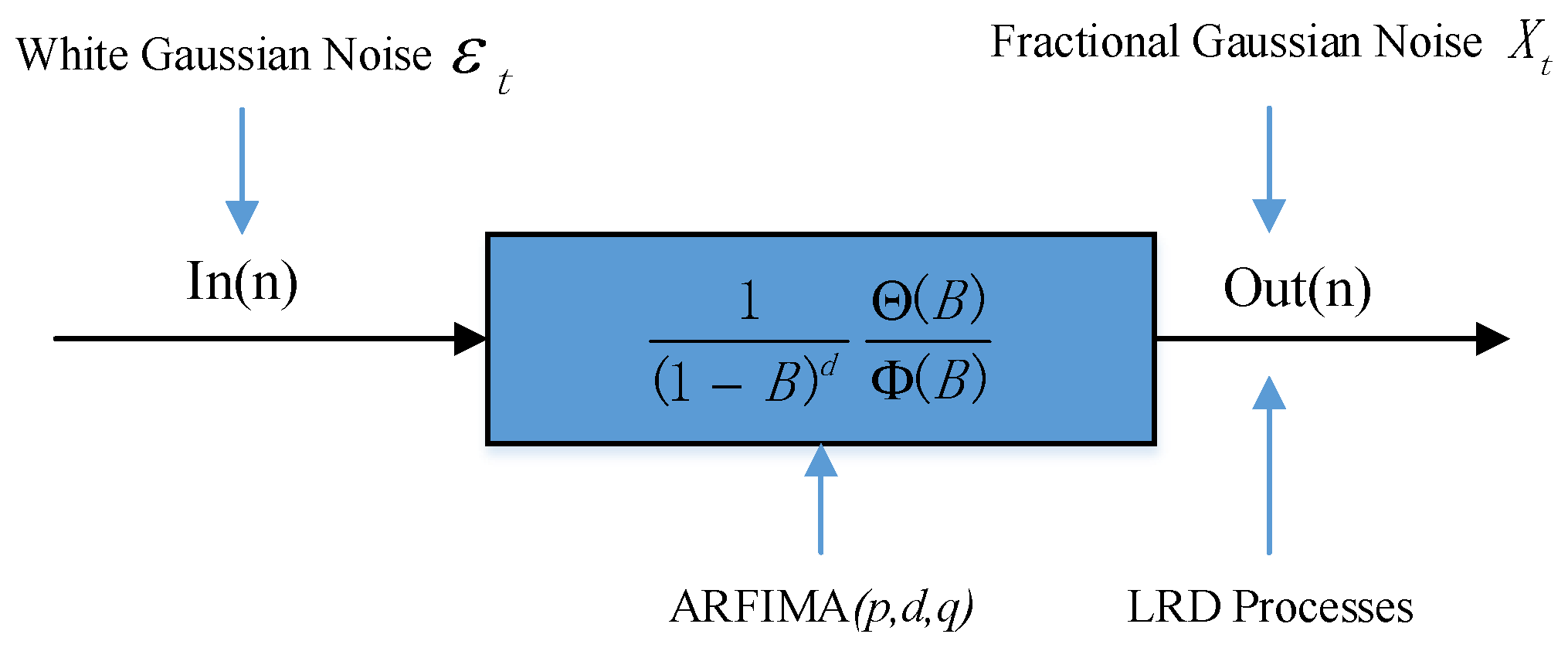
2.3. ARIMA and ARFIMA Model

The above AR and MA models can be generalized as follows [2]:
( 1 - i = 1 p ϕ i B i ) ( 1 - B ) d ( X t - μ ) = ( 1 + i = 1 q θ i B i ) ϵ t .
The above ( 1 - B ) d is called a difference operator d . The ARMA or ARIMA models can only capture the SRD property, since d is confined in the range of integer order. Therefore, in order to capture the LRD property of the fractional systems, the ARFIMA(p,d,q) model is thereby proposed accordingly. In fact, the operator can be defined in a natural way by using binomial expansion for any real number d with Gamma function:
( 1 - B ) d = k = 0 d k ( - B ) k = k = 0 Γ ( d + 1 ) Γ ( k + 1 ) Γ ( d + 1 - k ) ( - B ) k .
Many authors suggested the use of the fractionally ARIMA model by using a fractional difference operator rather than an integer one could better take into account this phenomenon of LRD [23]. Hosking et al. defined an extension of the ARIMA model, which allows for the possibility of stationary long-memory models [24]. Thus, the general form of ARIMA ( p , q , d ) process X t in Equation (7)—the ARFIMA(p,d,q) process is defined as:
Φ ( B ) ( 1 - B ) d X t = Θ ( B ) ε t ,
where d ( - 0 . 5 , 0 . 5 ) , and ( 1 - B ) d is defined as the fractional difference operator in Equation (8). ARFIMA ( p , d , q ) processes are widely used in modeling LRD time series, where p is the autoregressive order, q is the moving average order and d is the level of differencing [25]. The larger the value of d, the more closely it approximates a simple integrated series, and it may approximate a general integrated series better than a mixed fractional difference and ARMA model.
Figure 1 presents the discrete ARFIMA process that can be described as the output of the fractional-order system driven by a discrete white Gaussian noise (wGn). The ARFIMA ( p , d , q ) process is the natural generalization of the standard ARIMA or ARMA processes. In a fractionally differenced model, the difference coefficient d is a parameter to be estimated first [26]. The intensity of self-similar of ARFIMA is measured by a parameter d. For the finite variance process with fractional Gaussian noise, d has a closed relation with Hurst parameter H [3,26,27]:
d = H - 1 / 2 .
In addition, for the infinite variance process with fractional α -stable noise, d is related with Hurst and characteristic exponent α [18,22]:
d = H - 1 / α .
In this way, the parameter d may be chosen to model long-time effects, whereas p and q may be selected to model relatively short-time effects.

3. Review and Evaluation

ARFIMA ( p , d , q ) processes are widely used in modeling LRD time series, especially for the high frequency trading data, network traffic and hydrology dataset, etc. In practice, several time series exhibit LRD in their observations, leading to the development of a number of estimation and prediction methodologies to account for the slowly decaying autocorrelations. The ARFIMA process is one of the best-known classes of long-memory models. As introduced in Section 1, most statistical analysis programs have been embedded with ARFIMA models. A summary of the current software dealing with ARFIMA model analysis is as follows:
  • MATLAB applications
    MATLAB® (Matrix Laboratory) is a multi-paradigm numerical computing environment and fourth-generation programming language developed by MathWorks (Natick, MA 01760-2098, USA). The MATLAB applications are interactive applications written to perform technical computing tasks with the MATLAB scripting language from MATLAB File Exchange, through additional MATLAB products, and by users.
  • SAS software
    SAS (Statistical Analysis System) is a software suite developed by SAS Institute (Cary, NC 27513-2414, USA) for advanced analytics, multivariate analyses, business intelligence, data management, and predictive analytics.
  • R packages
    R packages and projects are contributed by RStudio (Boston, MA 02210, USA) team on CRAN (Comprehensive R Archive Network). R users are doing some of the most innovative and important work in science, education, and industry. It is a daily inspiration and challenge to keep up with the community and all it is accomplishing.
  • OxMetrics
    OxTM is an object-oriented matrix language with a comprehensive mathematical and statistical function library developed by Timberlake Consultants Limited (Richmond, Surrey TW9 3GA, UK). Many packages were written for Ox including software mainly for econometric modelling. The Ox packages for time series analysis and forecasting.
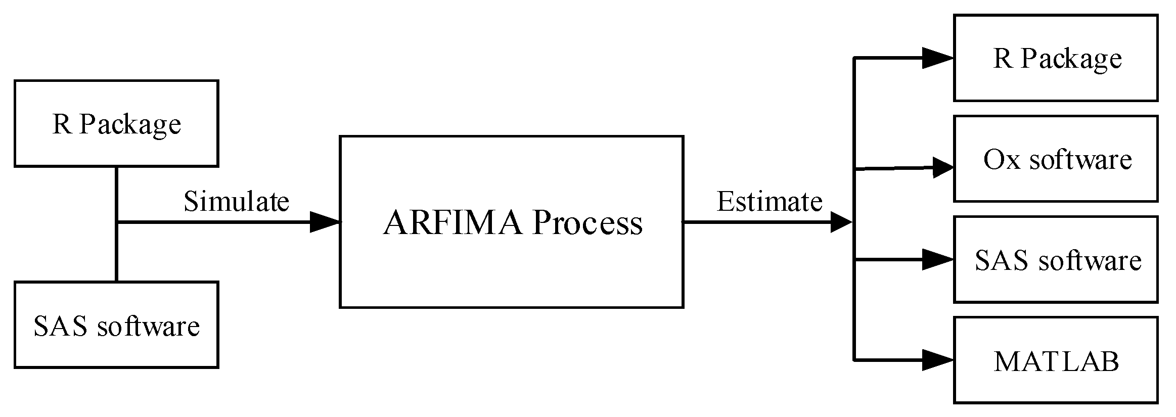
MATLAB codes are open-source applications where we could download, view and revise the codes if possible while other three are packaged and embedded in the software modules. In the following evaluation parts, we could clearly see the differences between them even with the same inputs. Four primary embedded functions concerning simulation, fractional difference filter, parameter estimation and forecast, are tested and evaluated for the ARFIMA processes in Table 1. It should be noted that the first two functions can be regarded as the forward problem solving systems, while the latter two are developed for the backward problem solving systems which are much more significant. In view of the above, this section can be divided into four parts.

3.1. Simulation

On the website of MATLAB Central, there are two files that can simulate ARFIMA processes. They are developed by Fatichi [28] and Caballero [29]. However, users cannot choose initial random seeds, that is, it can only simulate one certain series of ARFIMA process. The ARFIMA ( p , d , q ) estimator is developed by Inzelt, which is used for a linear stationary ARFIMA ( p , d , q ) process [30].
R is a freely available language and environment for statistical computing and graphics, which provides a wide variety of statistical and graphical techniques: linear and nonlinear modelling, statistical tests, time series analysis, classification, clustering, etc. Like the MATLAB Central, CRAN is a platform that stores identical, up-to-date, versions of code and documentation for R. There are several major packages concerning ARFIMA process according to the authors’ survey in Table 2.
The first two packages are used for the processing of ARFIMA processes, including Hurst fitting, calculation and fractional order difference and so on, while the latter two are mainly used for the parameter estimation of ARFIMA. The last package arfima is the most comprehensive tool that could simulate, estimate and predict the results of ARFIMA processes. In the paper, we use the last one package to compare with the other software.
SAS and R could also generate the ARFIMA process by defining the order of AR(p) and MA(q), setting the parameters ϕ , θ and d, respectively. In addition, the number of the initial random seeds could/should be set for the stochastic process. Random seeds are defined by the internal algorithms, which make the initial stochastic process a difference. Therefore, it may be a big difference if picking arbitrary seeds. In order to illustrate the above problems, we have generated the ARFIMA ( 1 , 0 . 4 , 1 ) process with d = 0 . 4 , ϕ = 0 . 5 , θ = - 0 . 1 and σ = 1 . Then, we set 100 different initial random seeds with 3000 observations and do the same estimation. It should be kept in mind that, even with the same simulation software that generates the processes, the estimation results could be a big difference in Figure 2. However, from the perspective of the sample-path analysis for the stochastic processes, this could be the advantage compared to the MATLAB ARFIMA applications, which can only generate one certain series (path). Furthermore, we have also found that the SAS software is somewhat better or “conservative”, while R software is more “aggressive” in Figure 2. We could check the comparisons below with dashed lines showing true values of parameters.
It should be also noted that, even with a certain series of the initial starting random seeds, the estimation results could also have quite a few variations. For example, we have set the fractional order d from 0 to 0.5, and do the simulation and estimation accordingly in MATLAB. It can be seen that the estimation d ^ is jumping up and down around the true values (red line) in Figure 3.
Here are some comments of this subsection:
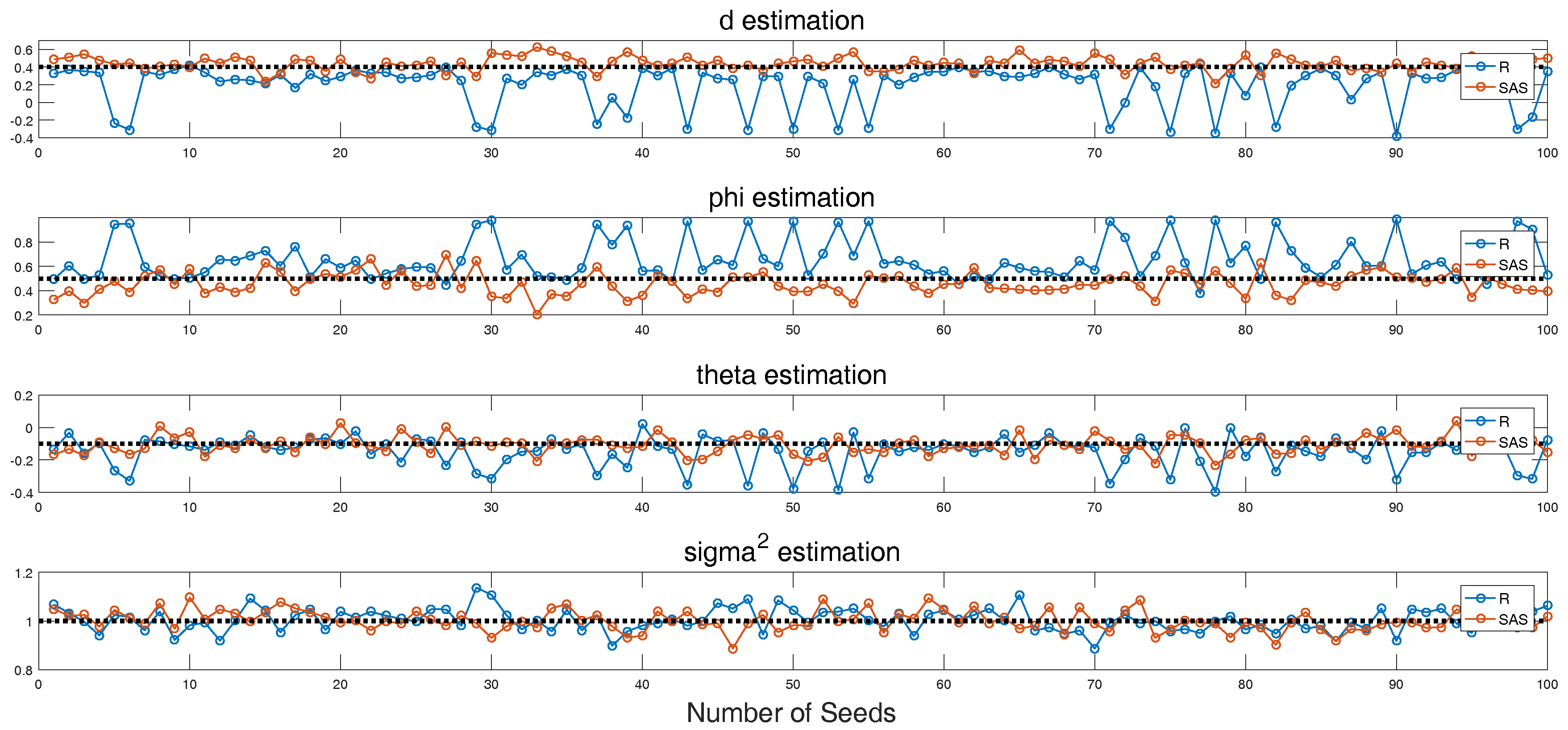
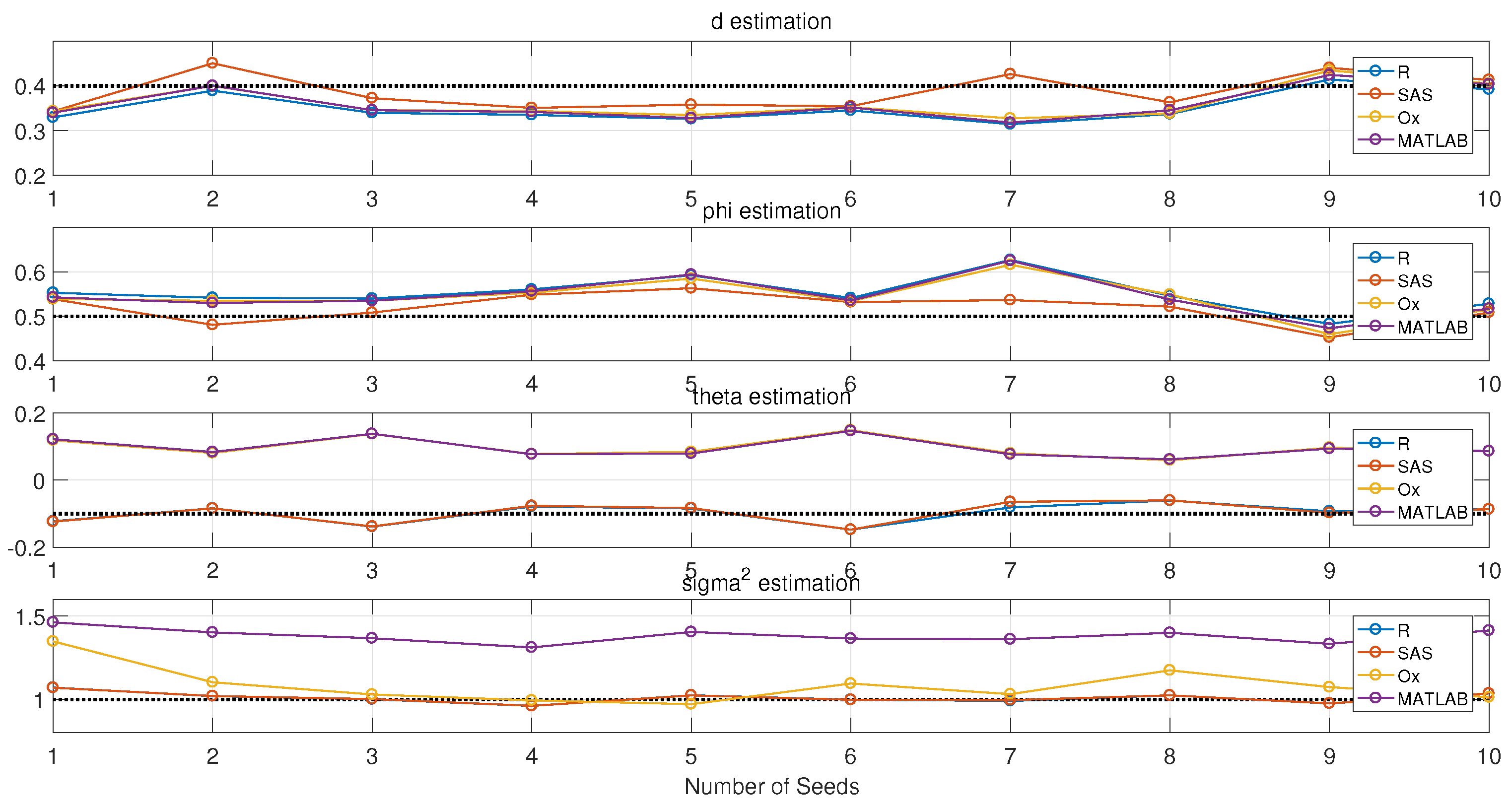
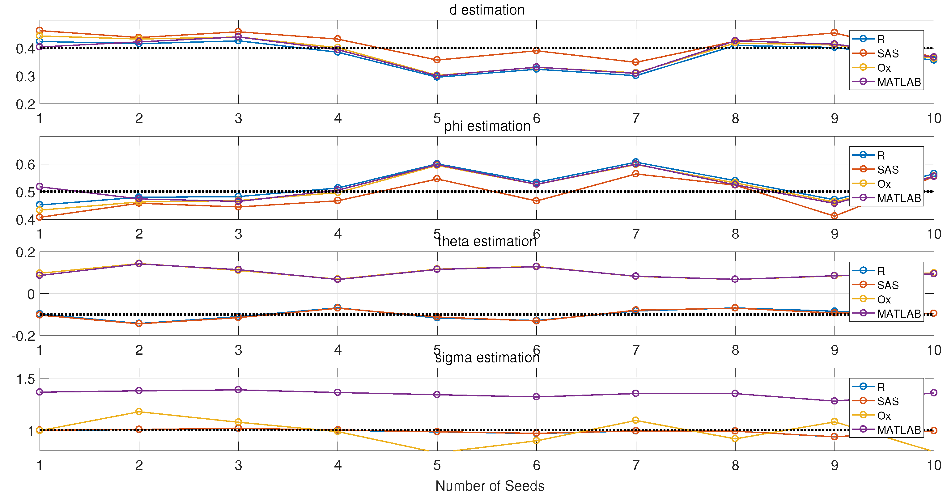
  • Estimation results also depend on the initial random seeds, even the series that are from their own simulations.
  • The test results may be different if not enough points/observations are generated. More than 300 points are preferred.
  • Estimation results may not be accurate if they only use one method. R should be more desirable to try first.

3.2. Fractional Order Difference Filter

Many time series signals contain trends, i.e., they are non-stationary. It is usually preferable to specify and remove the trends explicitly to get the smoothed or stationary data for the further analysis and modeling. According to the theory of Box–Jekins, an ARIMA model can be viewed as a “filter” that tries to separate the signal from the noise, and the signal is then extrapolated into the future to obtain forecasts [2]. Since the beginning of the 1980s, the long memory ARFIMA model has been introduced and investigated by many scholars especially for the parameter estimation problems. Shumway and Stoffer gave a brief overview of “long memory ARMA” models in [36]. This type of long memory model might be considered to use when the ACF of the series tapers slowly to 0 and spectral densities are unbounded at f = 0 . Jensen et al. derived an algorithm for the calculation of fractional differences based on circular convolutions method in [37]. In fact, there are a lot of estimation methods concerning fractional difference algorithms.
In some instances, however, we may see a persistent pattern of non-zero correlations that begins with a first lag correlation that is not close to 1. In these cases, models that incorporate “fractional differencing” may be useful. Therefore, differencing the time series data by using the approximated binomial expression of the long-memory filter is a prerequisite to estimates of the memory parameter in the ARFIMA ( p , d , q ) model. The user should not only set numeric vector of p and q, but also specify the order of the fractional difference filter. By passing through fractional order difference filter, the ARFIMA series will yield residuals that are uncorrelated and normally distributed with constant variance in Figure 4.
The sample ACF and partial autocorrelation function (PACF) are useful qualitative tools to assess the presence of autocorrelation at individual lags. The Ljung-Box Q-test is a more quantitative way to test for autocorrelation at multiple lags jointly [38]. The Ljung-Box test statistic is given by:
Q ( L ) = N ( N + 2 ) k = 1 L ρ ^ k 2 N - k ,
where N is the sample size, L is the number of autocorrelation lags, and ρ ( k ) is the sample autocorrelation at lag k. Under the null hypothesis, the asymptotic distribution of Q is chi-square with L degrees of freedom. If we use lbqtest function in the MATLAB Econometrics Toolbox, it returns the rejection decision and p-value for the hypothesis test. Similar functions Box.test of stats and ljung.wge of tswge are also available in the R package. p-values indicate the strength at which the test rejects the null hypothesis. If all of the p-values are larger than 0.01, there is strong evidence to accept the hypothesis that the residuals are not autocorrelated.
Thus, we have generated an ARFIMA(0,0.4,0) process in Figure 5 and use fractional order difference filter with the order d = 0 . 4 to filter the LRD property in Figure 6. It is obvious that, by passing through the fractional order difference filter, the slowly decaying property of LRD has been eliminated.
In order to evaluate residuals, p-values are used to quantify the goodness of fitting in Table 3.
Here are some comments of this subsection: all of the four programs above have fractional order operators to filter the LRD process successfully. In general, d is the parameter to be estimated first [26]. If we use the calculation defined by the Hurst method in Equations (10) and (11), d could probably be the fractional one. Therefore, the fractional order filter would be the primary tool to eliminate the LRD property or the heavy-tailedness in order to get the stationary series.
Meanwhile, however, the fractional order d is closely related to the Hurst parameter in Equations (10) and (11). There are more than ten methods to estimate Hurst parameters, R/S method, aggregated variance method, absolute value method, periodogram method, whittle method, Higuchi’s method, etc. These methods are mainly useful as simple diagnostic tools for LRD time series. These Hurst estimators have been introduced to analyze the LRD time series in [17,39,40]. Therefore, the results of Hurst estimators can be different if applying different methods. In addition, from Equation (8), it is interesting to note that there are infinite factorial series in the expansion of binomial expansion. In practice, we usually take the first three factorials for approximation. That is to say, the accuracy of differencing is also determined by how many factorials are used for approximation. Consequently, these different methods make the subsequent estimations differ from each other in the following sections.

3.3. Parameter Estimation
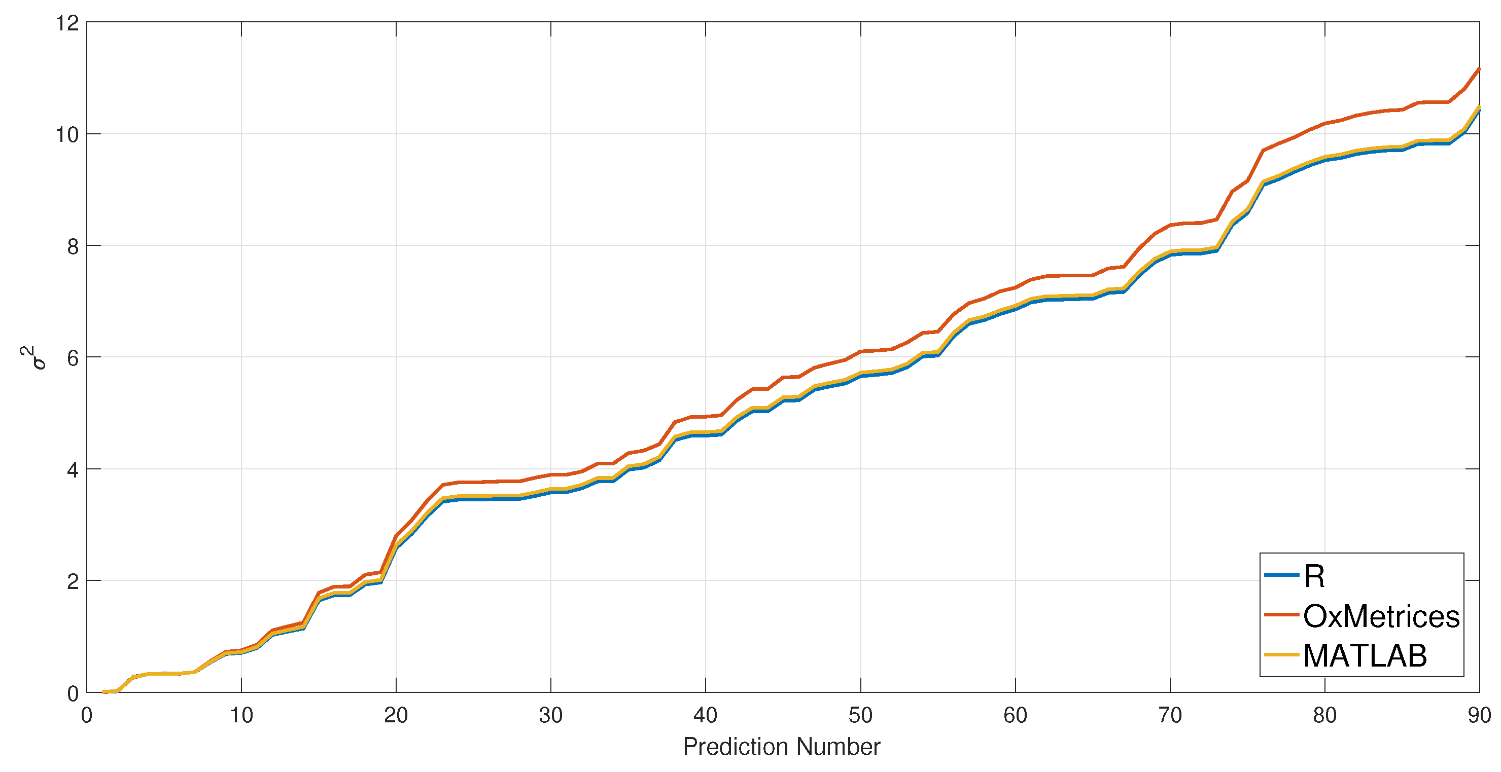
From Figure 2, we could see that, even though R and SAS can both simulate the ARFIMA processes, the properties of these processes are not the same mainly because of the distinctive random seeds defined by different software. Therefore, when reviewing and evaluating the accuracy of above software, the same ARFIMA series should be guaranteed first. Herein, we have proposed to use the following steps to compare the results in Figure 7. In addition, OxMetrics is the software that cannot generate ARFIMA simulation, but it can estimate and forecast ARFIMA-FIGARCH processes. MATLAB cannot generate multiple ARFIMA series for the same parameter combinations. We have thus used R and SAS to provide the ARFIMA series for the inputs of estimations.
Since we have received simulation results, the parameters of ARFIMA processes can be estimated and compared with true values (parameter setting values). First, we have used the simulation data from R software and have then used these three programs to do the estimation in Figure 8. Second, we have used SAS to do the same simulation and have then used the other three to do the estimation in Figure 9. Without loss of generality, we pick 10 groups of 3000 observations to see who could capture the accuracy.
Here are some comments from this subsection: from the above plots, it is very interesting to find that the estimation results of ARFIMA simulations are relatively accurate when they come from the same simulation data set. However, OxMetrics and MATLAB estimate the negative values of θ .
In order to further test whether the Ox and MATLAB can only return the negative values of θ or if they just return the inverse values. The parameters are set to the inverse values, accordingly, with ϕ = - 0 . 5 and θ = 0 . 2 ; while, in the previous test, they are ϕ = 0 . 5 and θ = - 0 . 1 , respectively. The result presented in Figure 10 validates the comments above.

3.4. Forecast

Simulation data could only be the auxiliary part of these software, since it can never be a powerful and useful tool for the ARFIMA process analysis if it cannot retrieve the estimation parameters from the real data with LRD. Moreover, the last and the most significant part of the ARFIMA process is to forecast and thereby predict the future behavior. Therefore, mean absolute percentage error (MAPE) values are used for the evaluation of the forecast results for the data from real life. The error square of the prediction results from different methods with the increasing number of predictions are illustrated in Figure 11:
σ t 2 = t = 1 n ( y t ^ - y t ) 2 .
Data description: Centered annual pinus longaeva tree ring width measurements at Mammoth Creek, Utah, USA from 0 A.D (anno Domini) to 1989 A.D with 1990 sampling points in time series [41,42]. The data can be divided into two parts: the first part with 1900 observations are used to estimate ARFIMA parameters, and the second part with 90 points are used for comparison with the prediction results from the fitted ARFIMA models. Finally, the results with the implemented methods that are applied to real-life time series are summarized in Table 4.
Here are some comments of this subsection:
  • d is the parameter to be estimated first when doing ARFIMA model fitting. Therefore, if the estimation of d is different for a certain time series, the following estimations for AR( Φ ) and MA( Θ ) will be different.
  • The ideal length (horizon) of predictions is within 30 steps. With the increasing steps of forecast, prediction errors are adding up. If a long range prediction series is required, R and MATLAB should be priorities for their smaller prediction errors.
  • Compared with other forecast results with true values in Table 4, R produces the minimum prediction errors and MAPE.

4. Summary of Selection Guidelines

Qualitative analysis as well as quantitative evaluations of the selected ARFIMA tools have been conducted in the previous sections. In order to make it easier for researchers from different backgrounds, we summarize the selection guidelines for the ARFIMA process modeling and analysis.
  • R and SAS software are priorities for the simulation of ARFIMA process, since they could define the initial seeds. R is one of the desirable tools for the estimation of ARFIMA process, since it has more than five packages including Hurst estimators, ACF plot, Quantile-Quantile (QQ) plot, white noise test and some LRD examples.
  • Estimation results of the ARFIMA process may be different if the number of observations is not large enough. Therefore, more than one estimation method should be used in order to guarantee the accuracy.
  • d is the parameter to be estimated first. All of this software could use fractional difference functions to filter the trend and thereafter stationarize time series data.
  • The ideal length (horizon) of predictions is within 30 steps. If a long range prediction series is required, R and MATLAB are the priorities for their smaller prediction errors.

5. Conclusions

Compared to the conventional integer order models that can only capture SRD, the ARFIMA model gives a better fitting result, especially for the data with the LRD property. Nowadays, some programs have been integrated with ARFIMA solutions. However, the final results of estimation and prediction could be different or even conflicting if choosing different methods. Therefore, a comprehensive review and evaluation of the numerical tools for the ARFIMA process is presented in the paper so as to provide some guidelines when choosing appropriate methods to do the time series analysis of LRD data. Through such efforts, it is hoped that an informative guidance is provided to the readers when they face the problem of selecting a numerical tool for a specific application.

Supplementary Materials

The MATLAB code, SAS code and R code for Section 3.1, Section 3.2, Section 3.3 and Section 3.4, and Ox code are available online at www.mdpi.com/2075-1680/6/2/16/s1.

Acknowledgments

We would like to thank the anonymous reviewers for their insightful comments on the paper.

Author Contributions

YangQuan Chen designed the experiment and Xi Zhang analyzed the data. Kai Liu performed the experiment and wrote the paper.

Conflicts of Interest

The authors declare no conflict of interest.

References

  1. Box, G.E.; Hunter, W.G.; Hunter, J.S. Statistics for Experimenters: An Introduction to Design, Data Analysis, and Model Building; John Wiley & Sons: Hoboken, NJ, USA, 1978; Volume 1. [Google Scholar]
  2. Box, G.E.; Jenkins, G.M.; Reinsel, G.C.; Ljung, G.M. Time Series Analysis: Forecasting and Control; John Wiley & Sons: Hoboken, NJ, USA, 2015. [Google Scholar]
  3. Sheng, H.; Chen, Y.; Qiu, T. Fractional Processes and Fractional-Order Signal Processing: Techniques and Applications; Springer Science & Business Media: New York, NY, USA, 2011. [Google Scholar]
  4. Mathai, A.M.; Saxena, R.K. The H-Function with Applications in Statistics and Other Disciplines; John Wiley & Sons: Hoboken, NJ, USA, 1978. [Google Scholar]
  5. Saxena, R.; Mathai, A.; Haubold, H. On fractional kinetic equations. Astrophys. Space Sci. 2002, 282, 281–287. [Google Scholar] [CrossRef]
  6. Saxena, R.; Mathai, A.; Haubold, H. On generalized fractional kinetic equations. Phys. A Stat. Mech. Its Appl. 2004, 344, 657–664. [Google Scholar] [CrossRef]
  7. Sun, R.; Chen, Y.; Li, Q. Modeling and prediction of Great Salt Lake elevation time series based on ARFIMA. In Proceedings of the International Design Engineering Technical Conferences and Computers and Information in Engineering Conference, Las Vegas, NV, USA, 4–7 September 2007; American Society of Mechanical Engineers: New York, NY, USA, 2007; pp. 1349–1359. [Google Scholar]
  8. Li, Q.; Tricaud, C.; Sun, R.; Chen, Y. Great Salt Lake surface level forecasting using FIGARCH model. In Proceedings of the International Design Engineering Technical Conferences and Computers and Information in Engineering Conference, Las Vegas, NV, USA, 4–7 September 2007; American Society of Mechanical Engineers: New York, NY, USA, 2007; pp. 1361–1370. [Google Scholar]
  9. Sheng, H.; Chen, Y. The modeling of Great Salt Lake elevation time series based on ARFIMA with stable innovations. In Proceedings of the International Design Engineering Technical Conferences and Computers and Information in Engineering Conference, San Diego, CA, USA, 30 August–2 September 2009; American Society of Mechanical Engineers: New York, NY, USA, 2009; pp. 1137–1145. [Google Scholar]
  10. Contreras-Reyes, J.E.; Palma, W. Statistical analysis of autoregressive fractionally integrated moving average models in R. Comput. Stat. 2013, 28, 2309–2331. [Google Scholar] [CrossRef]
  11. Baillie, R.T.; Chung, S. Modeling and forecasting from trend-stationary long memory models with applications to climatology. Int. J. Forecast. 2002, 18, 215–226. [Google Scholar] [CrossRef]
  12. Doornik, J.A.; Ooms, M. Computational aspects of maximum likelihood estimation of autoregressive fractionally integrated moving average models. Comput. Stat. Data Anal. 2003, 42, 333–348. [Google Scholar] [CrossRef]
  13. Doornik, J.A.; Ooms, M. A package for estimating, forecasting and simulating ARFIMA models: Arfima package 1.0 for Ox; Erasmus University: Rotterdam, The Netherlands, 1999. [Google Scholar]
  14. Doornik, J.A.; Ooms, M. Inference and forecasting for ARFIMA models with an application to US and UK inflation. Stud. Nonlinear Dyn. Econ. 2004, 8, 1208–1218. [Google Scholar] [CrossRef]
  15. Burnecki, K. Identification, Validation and Prediction of Fractional Dynamical Systems; Oficyna Wydawnicza Politechniki Wrocławskiej: Wroclaw, Poland, 2012. [Google Scholar]
  16. Hurst, H.E. Long-term storage capacity of reservoirs. Trans. Am. Soc. Civ. Eng. 1951, 116, 770–808. [Google Scholar]
  17. Ye, X.; Xia, X.; Zhang, J.; Chen, Y. Effects of trends and seasonalities on robustness of the Hurst parameter estimators. IET Signal Process. 2012, 6, 849–856. [Google Scholar] [CrossRef]
  18. Samorodnitsky, G.; Taqqu, M.S. Stable Non-Gaussian Random Processes: Stochastic Models with Infinite Variance; CRC Press: Boca Raton, FL, USA, 1994; Volume 1. [Google Scholar]
  19. Woodward, W.A.; Gray, H.L.; Elliott, A.C. Applied Time Series Analysis with R, 2nd ed.; CRC Press: Boca Raton, FL, USA, 2016. [Google Scholar]
  20. Kale, M.; Butar, F.B. Fractal analysis of time series and distribution properties of Hurst exponent. J. Math. Sci. Math. Educ. 2011, 5, 8–19. [Google Scholar]
  21. Karasaridis, A.; Hatzinakos, D. Network heavy traffic modeling using α-stable self-similar processes. IEEE Trans. Commun. 2001, 49, 1203–1214. [Google Scholar] [CrossRef]
  22. Sheng, H.; Chen, Y. FARIMA with stable innovations model of Great Salt Lake elevation time series. Signal Process. 2011, 91, 553–561. [Google Scholar] [CrossRef]
  23. Granger, C.W.; Joyeux, R. An introduction to long-memory time series models and fractional differencing. J. Time Ser. Anal. 1980, 1, 15–29. [Google Scholar] [CrossRef]
  24. Hosking, J.R. Fractional differencing. Biometrika 1981, 68, 165–176. [Google Scholar] [CrossRef]
  25. Brockwell, P.J.; Davis, R.A. Time Series: Theory and Methods; Springer Science & Business Media: New York, NY, USA, 2013. [Google Scholar]
  26. Reisen, V.; Abraham, B.; Lopes, S. Estimation of parameters in ARFIMA processes: A simulation study. Commun. Stat.-Simul. Comput. 2001, 30, 787–803. [Google Scholar] [CrossRef]
  27. Reisen, V.A. Estimation of the fractional difference parameter in the ARIMA (p, d, q) model using the smoothed periodogram. J. Time Ser. Anal. 1994, 15, 335–350. [Google Scholar] [CrossRef]
  28. Fatichi, S. ARFIMA Simulations. Available online: https://www.mathworks.com/matlabcentral/fileexchange/25611-arfima-simulations/content/ARFIMASIM.m (accessed on 15 June 2017).
  29. Caballero, C.V.R. ARFIMA(p, d, q). Available online: https://www.mathworks.com/matlabcentral/fileexchange/53301-arfima-p-d-q-/content/dgparfima.m (accessed on 15 June 2017).
  30. Inzelt, G. ARFIMA(p, d, q) Estimator. Available online: https://www.mathworks.com/matlabcentral/fileexchange/30238-arfima-p-d-q--estimator (accessed on 15 June 2017).
  31. Constantine, W.; Percival, D.; Constantine, M.W.; Percival, D.B. The Fractal Package for R. Available online: https://cran.r-project.org/web/packages/fractal/fractal.pdf (accessed on 15 June 2017).
  32. Maechler, M.; Fraley, C.; Leisch, F. The Fracdiff Package for R. Available online: https://cran.r-project.org/web/packages/fracdiff/fracdiff.pdf (accessed on 15 June 2017).
  33. Contreras-Reyes, J.E.; Goerg, G.M.; Palma, W. The Afmtools Package for R. Available online: http://www2.uaem.mx/r-mirror/web/packages/afmtools/afmtools.pdf (accessed on 15 June 2017).
  34. Kraft, P.; Weber, C.; Lebo, M. The ArfimaMLM Package for R. Available online: https://cran.r-project.org/web/packages/ArfimaMLM/ArfimaMLM.pdf (accessed on 15 June 2017).
  35. Veenstra, J.Q.; McLeod, A. The Arfima Package for R. Available online: https://cran.r-project.org/web/packages/arfima/arfima.pdf (accessed on 15 June 2017).
  36. Shumway, R.H.; Stoffer, D.S. Time Series Analysis and Its Applications: With R Examples; Springer Science & Business Media: New York, NY, USA, 2010. [Google Scholar]
  37. Jensen, A.N.; Nielsen, M.Ø. A fast fractional difference algorithm. J. Time Ser. Anal. 2014, 35, 428–436. [Google Scholar] [CrossRef]
  38. Ljung, G.M.; Box, G.E. On a measure of lack of fit in time series models. Biometrika 1978, 65, 297–303. [Google Scholar] [CrossRef]
  39. Sheng, H.; Chen, Y.; Qiu, T. On the robustness of Hurst estimators. IET Signal Process. 2011, 5, 209–225. [Google Scholar] [CrossRef]
  40. Chen, Y.; Sun, R.; Zhou, A. An improved Hurst parameter estimator based on fractional Fourier transform. In Proceedings of the International Design Engineering Technical Conferences and Computers and Information in Engineering Conference, Las Vegas, NV, USA, 4–7 September 2007; American Society of Mechanical Engineers: New York, NY, USA, 2007; pp. 1223–1233. [Google Scholar]
  41. Palma, W. Long-Memory Time Series: Theory and Methods; John Wiley & Sons: Hoboken, NJ, USA, 2007; Volume 662. [Google Scholar]
  42. Palma, W.; Olea, R. An efficient estimator for locally stationary Gaussian long-memory processes. Ann. Stat. 2010, 38, 2958–2997. [Google Scholar] [CrossRef]
Figure 1. ARFIMA model.
Axioms 06 00016 g001
Figure 2. Estimation results of SAS and R.
Axioms 06 00016 g002
Figure 3. Comparison of d ^ and d.
Axioms 06 00016 g003
Figure 4. Fractional order difference of the ARFIMA ( 0 , 0 . 4 , 0 ) process.
Axioms 06 00016 g004
Figure 5. Simulation of ARFIMA ( 0 , 0 . 4 , 0 ) process.
Axioms 06 00016 g005
Figure 6. ARFIMA(0,0.4,0) process passing through the fractional difference filter.
Axioms 06 00016 g006
Figure 7. Simulation and estimation of the ARFIMA process.
Axioms 06 00016 g007
Figure 8. Parameter estimation with different methods (R simulation inputs).
Axioms 06 00016 g008
Figure 9. Parameter estimation with different methods (SAS simulation inputs).
Axioms 06 00016 g009
Figure 10. Parameter estimation with different methods (R simulation inputs).
Axioms 06 00016 g010
Figure 11. Prediction comparison with different methods.
Axioms 06 00016 g011
Table 1. Numerical tools for the ARFIMA process.
ProceduresMATLABRSASOxMetrics
Simulation *
Fractional Difference
Parameter Estimation
Forecast
* means it can simulate ARFIMA processes, but cannot choose or define the initial seeds.
Table 2. Comparison of ARFIMA packages in R.
PackageAuthorRelease DateTypical FunctionsRequirements
fractalWilliam Constantine et al. [31]2016-05-21hurstSpecR (≥ 3.0.2)
fracdiffMartin Maechler et al. [32]2012-12-02fracdifflongmemo, urca
afmtoolsJavier E. Contreras-Reyes et al. [33]2012-12-28arfima.whittleR (≥ 2.6.0), polynom fracdiff, hypergeo, sandwich, longmemo
ArfimaMLMPatrick Kraft et al. [34]2015-01-21arfimaMLMR (≥ 3.0.0), fractal
arfimaJustin Q. Veenstra et al. [35]2015-12-31arfimaR (≥ 2.14.0), ltsa
Table 3. Fractional filters.
SoftwareMATLABRSASOx
Functiond_filterdiffseriesfdiffracdiff
p-values with 1,5,10,15 lags0.07100.099980.10620.0862
0.22530.23950.24140.2114
0.58500.53200.51980.5898
0.53300.45710.44730.5473
Table 4. Parameter estimations and forecast comparisons.
NumberParametersRSASOxMetricesMATLAB
1mu0.9833N/A (Not Applicable)0.987990.9878
2d0.16700.14796240.2820870.2313
3ar0.90701190.8939677−0.2542650.6473
4ma0.86038110.83187870.186980.6393
5sigma0.10781730.10734170.12460.1163
6p value Lag10.9195N/A0.77094580.9101
7p value Lag50.6369N/A0.3413240.6959
8p value Lag100.8659N/A0.43679250.9037
9p value Lag150.6491N/A0.62295420.6776
10LogLikelihood2117.2241851.5512−570.5991162.527
11MAPE28.95N/A29.3629.02

