Complexity and Chaos Analysis for Two-Dimensional Discrete-Time Predator–Prey Leslie–Gower Model with Fractional Orders

Abstract

The paper introduces a novel two-dimensional fractional discrete-time predator–prey Leslie–Gower model with an Allee effect on the predator population. The model’s nonlinear dynamics are explored using various numerical techniques, including phase portraits, bifurcations and maximum Lyapunov exponent, with consideration given to both commensurate and incommensurate fractional orders. These techniques reveal that the fractional-order predator–prey Leslie–Gower model exhibits intricate and diverse dynamical characteristics, including stable trajectories, periodic motion, and chaotic attractors, which are affected by the variance of the system parameters, the commensurate fractional order, and the incommensurate fractional order. Finally, we employ the 0–1 method, the approximate entropy test and the $C_0$ algorithm to measure complexity and confirm chaos in the proposed system.

1. Introduction

Over the past few years, researchers have been giving more and more attention to biological models, particularly those related to predator–prey interactions. These models are important in the field of biology and have been extensively explored in both mathematical biology and ecology. Through the analysis of these models, researchers have discovered a range of complex dynamics, including bifurcations, limit cycles, and chaotic behaviour. While continuous-time systems have been extensively studied, discrete-time systems have not received as much attention. However, discrete-time models have unique dynamic properties and can be used to represent several practical issues that occur in the biological world. Discrete-time systems are particularly useful in cases where the dynamics of a system change rapidly over time, or where the system is subject to discrete events or inputs. Due to these characteristics, studying discrete systems is essential and has resulted in notable advances in various fields such as mathematics, biology, engineering, ecology and others.

Discrete fractional calculus is an area of mathematics that looks at discrete fractional calculus analogs. Fractional calculus is an extension of classical calculus that works with derivatives and integrals of non-integer orders. It has many uses in different domains including engineering, physics, and economics, among others. Over the last several years, it has garnered significant considerable interest as a result of its potential applications in various fields such as image processing, signal processing, and data analysis. The study of discrete fractional calculus involves the development of new mathematical tools and techniques for analyzing and manipulating discrete fractional operators, and the investigation of their properties and applications. In recent times, there has been a surge of publications addressing the topic of discrete-time fractional calculus. These publications put forth numerous discrete-time fractional operators, stability analyses, and theoretical results [1,2,3,4,5]. As a consequence of these works, there has been an increase in the development of commensurate and incommensurate fractional discrete chaotic systems, as seen in [6,7,8,9,10,11,12,13] and references therein. Additionally, various control strategies and synchronization schemes have been proposed to synchronize different fractional chaotic maps [14,15,16,17,18].

Recently, a considerable number of researchers have investigated the dynamical behaviors of discrete models. However, only a limited amount of literature exists that focuses on analyzing the dynamics of discrete-time predator–prey systems [19,20,21]. For instance, the bifurcation analysis and hybrid control of discrete predator–prey model have been studied by Yuan and Yang in [22]. The chaos control of the discrete modified predator–prey Leslie–Gower harvesting system has been analyzed by Ajaz et al. in [23]. In [24], the author has explored the chaos and complexity in a discrete-time prey-predator model. Khan et al. in [25] discussed the Neimark–Sacker bifurcations and global dynamics in a discrete prey-predator Leslie model, while Vinoth et al. [26] investigated the dynamic behaviors of a new Leslie–Gower discrete-time system with the Allee impact in predator populations. The Allee effect is a biological phenomenon that has been named after Allee, who produced a comprehensive account of it. This statement indicates the existence of a direct correlation between the size of a population and its per capita growth rate [27]. Most of the research above has focused on classical integer-order models. As far as current literature indicates, there have been no research contributions that specifically analyze the behaviours of a fractional-order discrete-time predator–prey Leslie–Gower system with the influence of the Allee effect in predator population. Therefore, the chaotic dynamical behaviours of such a system that utilizes fractional difference operators possessing both commensurate and incommensurate orders is an appealing field for further study.

Based on the discussion presented earlier, the objective of this paper is to investigate and analyze the rich chaotic dynamics of a newly proposed commensurate fractional-order fractional discrete-time predator–prey Leslie–Gower system and incommensurate fractional-order fractional discrete-time predator–prey Leslie–Gower system by taking the Allee parameter as a bifurcation parameter. The basic properties of this fractional model will be studied using certain theoretical and numerical analyses. Furthermore, we will use the approximate entropy test and $C_0$ algorithm to measure the complexity and validate the presence of chaos in the proposed system. Finally, we will conclude the study by summarizing the most significant findings obtained in the article.

The paper is organized as follows. In Section 2, we provide the mathematical formulation of the model utilizing the Caputo-like operator. In Section 3, we delve the fundamental properties of the model through numerical theoretical and analyses. In Section 4, we employ the 0–1 method, the approximate entropy test and $C_0$ algorithm to measure complexity and confirm the existence of chaos within the suggested model. Finally, the paper concludes by summarizing the most noteworthy outcomes obtained throughout the study.

2. Model Description of the Fractional Discrete System

Subject to the continuous predator–prey model of modified Leslie–Gower given in [28], Vinoth et al. [26] describes the following fractional discrete-time predator–prey Leslie–Gower system with the influence of the Allee effect in Predator Population:

$$\begin{array}{cc}\hfill z_1(r+1)& =z_1\left(r\right)exp\left[{\delta }_1-\alpha z_1\left(r\right)-\frac{h_1{z}_2\left(r\right)}{z_1\left(r\right)+b}\right],\hfill \\ \hfill z_2(r+1)& =z_2\left(r\right)exp\left[\frac{{\delta }_2{z}_2\left(r\right)}{z_2\left(r\right)+m}-\frac{h_2{z}_2\left(r\right)}{z_1\left(r\right)+c}\right],\hfill \end{array}$$

(1)

where $z_1\le 0$ and $z_2\le 0$ denote the population sizes. $\frac{z_2\left(r\right)}{m+z_2\left(r\right)}$ is the Allee effect term and $m>0$ represents the severity of Allee effect in the predator population. ${\delta }_1,{\delta }_2,\alpha ,h_1,h_2,b,c$ are positive constant parameters. In our work, we intend to use the Caputo-like operator to obtain a new fractional discrete predator–prey model. First, we formulate the first-order differences of the fractional discrete-time predator–prey Leslie–Gower model as follows:

$$\begin{array}{cc}\hfill \Delta z_1\left(r\right)& =z_1\left(r\right)exp\left[{\delta }_1-\alpha z_1\left(r\right)-\frac{h_1{z}_2\left(r\right)}{z_1\left(r\right)+b}\right]-z_1\left(r\right),\hfill \\ \hfill \Delta z_2\left(r\right)& =z_2\left(r\right)exp\left[\frac{{\delta }_2{z}_2\left(r\right)}{z_2\left(r\right)+m}-\frac{h_2{z}_2\left(r\right)}{z_1\left(r\right)+c}\right]-z_2\left(r\right),\hfill \end{array}$$

(2)

Next, we use the difference operator ${}^c{\Delta }_a^{\vartheta }$ to produce a novel fractional discrete-time predator–prey Leslie–Gower model with the Allee effect in predator population. The formulation of the mathematical form of the system is as follows:

$$\begin{array}{cc}\hfill {}^c{\Delta }_a^{\vartheta }{z}_1\left(r\right)& =z_1(r+\vartheta -1)exp\left[{\delta }_1-\alpha z_1(r+\vartheta -1)-\frac{h_1{z}_2(r+\vartheta -1)}{z_1(r+\vartheta -1)+b}\right]-z_1(r+\vartheta -1),\hfill \\ \hfill {}^c{\Delta }_a^{\vartheta }{z}_2\left(r\right)& =z_2(r+\vartheta -1)exp\left[\frac{{\delta }_2{z}_2(r+\vartheta -1)}{z_2(r+\vartheta -1)+m}-\frac{h_2{z}_2(r+\vartheta -1)}{z_1(r+\vartheta -1)+c}\right]-z_2(r+\vartheta -1).\hfill \end{array}$$

(3)

The Caputo-like difference operator ${}^C{\Delta }_a^{\vartheta }$ can be given by [4]

$$\begin{array}{cc}\hfill {}^C{\Delta }_a^{\vartheta }\chi \left(r\right)& ={\Delta }_a^{-(m-\vartheta )}{\Delta }^m\chi \left(r\right).\hfill \end{array}$$

(4)

$r\in {\left(\mathbb{N}\right)}_{a-\vartheta +m}$ and $m=\lceil \vartheta \rceil +1$. ${\Delta }_a^{-\vartheta }$ is fractional sum which is defined as [2]

$${\Delta }_a^{-\vartheta }\chi \left(r\right)=\frac{1}{\mathsf{\Gamma }\left(\vartheta \right)}\sum _{k=\vartheta }^{r-\vartheta }{(r-k-1)}^{(\vartheta -1)}\chi \left(k\right),r\in {\left(\mathbb{N}\right)}_{m+\vartheta },\vartheta >0$$

(5)

Now, the following theorem will be presented, which will help us to gain the derivation of the numerical expression for the fractional discrete-time predator–prey Leslie–Gower system (3):

Theorem 1

([29]). The solution of the following system

$$\left\{\begin{array}{c}{}^C{\Delta }_a^{\vartheta }\chi \left(r\right)=g(r-1+\vartheta ,\chi (r-1+\vartheta ))\hfill \\ {\Delta }^j\chi \left(a\right)={\chi }_j,m=\lceil \vartheta \rceil +1,j=0,1,\dots ,m-1,\hfill \end{array}\right.$$

(6)

is given by

$$\chi \left(r\right)={\chi }_0\left(a\right)+\frac{1}{\mathsf{\Gamma }\left(\vartheta \right)}\sum _{k=d+m-\vartheta }^{r-\vartheta }{(r-k-1)}^{(\vartheta -1)}g(k+\vartheta -1,\chi (k+\vartheta -1)),r\in {\mathbb{N}}_{a+m},$$

(7)

where

$${\chi }_0\left(a\right)=\sum _{j=0}^{m-1}\frac{{(r-a)}^j}{\mathsf{\Gamma }(n+1)}{\Delta }^j\chi \left(a\right).$$

(8)

Remark 1.

Take $a=0$, $m=1$, $j=k+\vartheta -1$ and ${(r-k-1)}^{(\vartheta -1)}=\frac{\mathsf{\Gamma }(r-k)}{\mathsf{\Gamma }(r-k-\vartheta +1)}$, the numerical expression (7) can be written for $\vartheta \in (0,1]$ as follows:

$$\chi \left(r\right)=\chi \left(0\right)+\frac{1}{\mathsf{\Gamma }\left(\vartheta \right)}\sum _{j=0}^{r-1}\frac{\mathsf{\Gamma }(r-n+\vartheta -1)}{\mathsf{\Gamma }(r-n)}g\left(j,\chi \left(j\right)\right).$$

(9)

3. Nonlinear Dynamics of the Fractional Discrete-Time Predator–Prey Leslie–Gower Model

This section will analyze the behaviour of the fractional discrete-time predator–prey Leslie–Gower model with an Allee effect on the predator population. The analysis will be conducted in two cases: commensurate, incommensurate. Various numerical analysis techniques, including the display of phase portraits, the plot of bifurcations, and the estimations of maximum Lyapunov exponents ($L{E}_{max}$), will be utilized. To calculate the maximum Lyapunov exponents of the model’s attractors, we will use the Jacobian matrix algorithm introduced in [30].

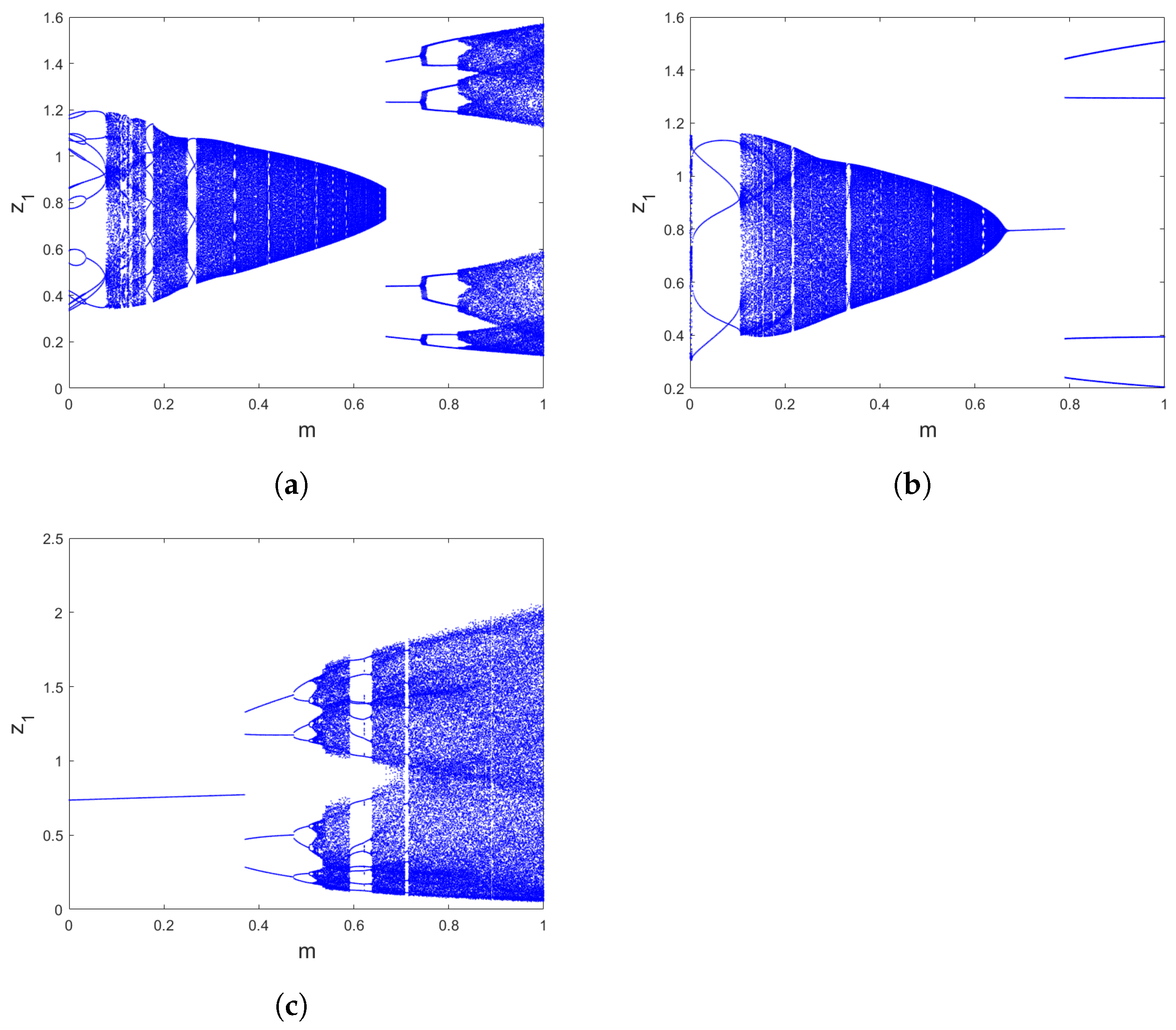
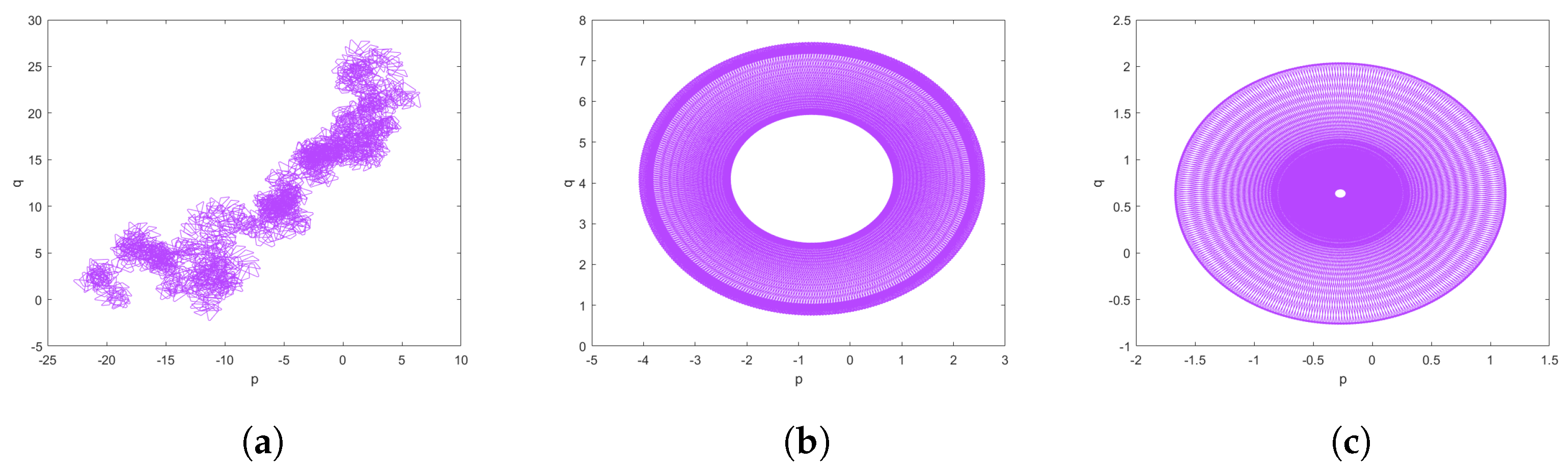
3.1. Commensurate Order FDNN Model

Here, we will focus on describing the features of a suggested commensurate fractional discrete-time predator–prey Leslie–Gower model with an Allee effect on the predator population (3). It is worth noting that a commensurate order system consists of equations with the same fractional orders. In light of this, we will now provide the numerical formula, which is derived from Theorem 1, as follows:

$$\left\{\begin{array}{c}{z}_1(r+1)=z_1\left(0\right)+{\displaystyle \sum _{k=0}^n}\frac{\mathsf{\Gamma }(r-1-k+\vartheta )}{\mathsf{\Gamma }\left(\vartheta \right)\mathsf{\Gamma }(r-k)}\left(z_1\left(k\right)exp\left[{\delta }_1-\alpha z_1\left(k\right)-\frac{h_1{z}_2\left(k\right)}{z_1\left(k\right)+b}\right]-z_1\left(k\right)\right),\hfill \\ z_2(r+1)=z_2\left(0\right)+{\displaystyle \sum _{k=0}^n}\frac{\mathsf{\Gamma }(r-1-k+\vartheta )}{\mathsf{\Gamma }\left(\vartheta \right)\mathsf{\Gamma }(r-k)}\left(z_2\left(k\right)exp\left[\frac{{\delta }_2{z}_2\left(k\right)}{z_2\left(k\right)+m}-\frac{h_2{z}_2\left(k\right)}{z_1\left(k\right)+c}\right]-z_2\left(k\right)\right),r=1,2,\cdots .\hfill \end{array}\right.$$

(10)

where $z_1\left(0\right)$ and $z_2\left(0\right)$ are the initial conditions (I.C). Setting the parameters system ${\delta }_1=3.3$, ${\delta }_2=1$, $\alpha =3.3$, $h_1=1.2$, $h_2=0.525$, $b=2.5$, $c=0.5$, $m=0.9$ and I.C $(z_1\left(0\right),z_2\left(0\right))=(1,2)$, The bifurcation diagrams are used to depict the variations in the behaviours of the fractional discrete predator–prey model (3) as the commensurate order $\vartheta$ is varied with step size $\Delta \vartheta =0.00003$. Figure 1 depicts the bifurcation and the ($L{E}_{max}$). The Lyapunov exponents are estimated by means of the jacobian matrix algorithm (see [30]), which are computed in a manner similar to that used to determine the states in the fractional discrete system (3). We define the tangent map $J_i$ as:

$$J_m=\left(\begin{array}{cc}{a}_1\left(m\right)& a_2\left(m\right)\\ b_1\left(m\right)& b_2\left(m\right)\end{array}\right)$$

(11)

where

$$\left\{\begin{array}{cc}{a}_1\left(m\right)=a_1\left(0\right)+\frac{1}{\mathsf{\Gamma }\left(\vartheta \right)}\sum _{j=0}^{m-1}\frac{\mathsf{\Gamma }(m-j-1+\vartheta )}{\mathsf{\Gamma }(m-j)}[\hfill & \left(a_1\left(j\right)+z_1\left(j\right)\left(-\alpha a_1\left(j\right)-\frac{h_1{b}_1\left(j\right)(z_1\left(j\right)+b)-h_1{a}_1\left(j\right)z_2\left(j\right)}{{(z_1\left(j\right)+b)}^2}\right)\right)\hfill \\ & exp\left({\delta }_1-\alpha z_1\left(k\right)-\frac{h_1{z}_2\left(k\right)}{z_1\left(k\right)+b}\right)-a_1\left(j\right)],\hfill \\ a_2\left(m\right)=a_2\left(0\right)+\frac{1}{\mathsf{\Gamma }\left(\vartheta \right)}\sum _{j=0}^{m-1}\frac{\mathsf{\Gamma }(m-j-1+\vartheta )}{\mathsf{\Gamma }(m-j)}[\hfill & \left(a_2\left(j\right)+z_1\left(j\right)\left(-\alpha a_2\left(j\right)-\frac{h_1{b}_2\left(j\right)(z_1\left(j\right)+b)-h_1{a}_2\left(j\right)z_2\left(j\right)}{{(z_1\left(j\right)+b)}^2}\right)\right)\hfill \\ & exp\left({\delta }_1-\alpha z_1\left(k\right)-\frac{h_1{z}_2\left(k\right)}{z_1\left(k\right)+b}\right)-a_2\left(j\right)],\hfill \\ b_1\left(m\right)=b_1\left(0\right)+\frac{1}{\mathsf{\Gamma }\left(\vartheta \right)}\sum _{j=0}^{m-1}\frac{\mathsf{\Gamma }(m-j-1+\vartheta )}{\mathsf{\Gamma }(m-j)}[\hfill & \left(b_1\left(j\right)+z_2\left(j\right)\left(\frac{{\delta }_2{b}_1\left(j\right)m)}{{(z_2\left(j\right)+m)}^2}-\frac{h_1{b}_1\left(j\right)(z_1\left(j\right)+c)-h_1{a}_1\left(j\right)z_2\left(j\right)}{{(z_1\left(j\right)+c)}^2}\right)\right)\hfill \\ & exp\left(\frac{{\delta }_2{z}_2\left(k\right)}{z_2\left(k\right)+m}-\frac{h_2{z}_2\left(k\right)}{z_1\left(k\right)+c}\right)-b_1\left(j\right)],\hfill \\ b_2\left(m\right)=b_2\left(0\right)+\frac{1}{\mathsf{\Gamma }\left(\vartheta \right)}\sum _{j=0}^{m-1}\frac{\mathsf{\Gamma }(m-j-1+\vartheta )}{\mathsf{\Gamma }(m-j)}[\hfill & \left(b_2\left(j\right)+z_2\left(j\right)\left(\frac{{\delta }_2{b}_2\left(j\right)m)}{{(z_2\left(j\right)+m)}^2}-\frac{h_1{b}_2\left(j\right)(z_1\left(j\right)+c)-h_1{a}_2\left(j\right)z_2\left(j\right)}{{(z_1\left(j\right)+c)}^2}\right)\right)\hfill \\ & exp\left(\frac{{\delta }_2{z}_2\left(k\right)}{z_2\left(k\right)+m}-\frac{h_2{z}_2\left(k\right)}{z_1\left(k\right)+c}\right)-b_1\left(j\right)],\hfill \end{array}\right.$$

(12)

with

$$\left(\begin{array}{cc}{a}_1\left(0\right)& a_2\left(0\right)\\ b_1\left(0\right)& b_2\left(0\right)\end{array}\right)=\left(\begin{array}{cc}1& 0\\ 0& 1\end{array}\right)$$

(13)

Then, the Lyapunov exponents can be given by:

$$L{E}_{\kappa }=\underset{m\to \infty }{lim}\frac{1}{m}ln\left|{\lambda }_{\kappa }^{\left(m\right)}\right|,\mathrm{for}\kappa =1,2.$$

(14)

where ${\lambda }_{\kappa }^{\left(m\right)}$ is the eigenvalue of the Jacobian matrix $J_m$.

Since the inherent complexity of accurate predictions of the system’s behaviour using analytical methods is challenging, numerical approximations are often necessary. One such approach involves using MATLAB R2022a software. From Figure 1, we can see that upon changing the commensurate order $\vartheta$, the system (3) exhibits different dynamics involving chaos and periodic motion. In particular, when $\vartheta$ takes larger values, the trajectories are chaotic. Moreover, when the commensurate order decreases, periodic windows with 5-period orbits appear and the model becomes stable at $\vartheta \in [0.9945,0.9956]$. If $\vartheta <0.9945$, the trajectories of the model lose their stability and the chaotic motions occur again where $L{E}_{max}$ is negative. If $\vartheta$ continues to decrease, the transition states are shown and then the commensurate fractional discrete predator–prey model with an Allee effect on the predator population converges toward infinity. Next, we generated three bifurcations of (3) with respect to the varying values of m, as illustrated in Figure 2. The plotted diagrams correspond to the commensurate values $\vartheta =0.99,\vartheta =0.995$ and $\vartheta =0.998$. We notice that the states of the commensurate fractional discrete-time predator–prey Leslie–Gower model (3) are affected by the system parameter m and the commensurate fractional order $\vartheta$. For instance, when the order $\vartheta$ increases, the chaotic region shrinks and more periodic states are observed. For completeness, to have a comprehensive comprehension of the aforementioned characteristics, Figure 3 portrays the discrete time evolution of the states $z_1$ and $z_2$ of the proposed commensurate system (3) while Figure 4 depicts the results of different phase portraits for $\vartheta =0.99,\vartheta =0.9947,\vartheta =0.995,\vartheta =0.9956,\vartheta =0.998$ and $\vartheta =1$. It is clear that the trajectories of the proposed commensurate fractional discrete model change their motion between chaotic motion and periodic ones when the commensurate order $\vartheta$ varied. These numerical computations indicate that the predator–prey discrete-time Leslie–Gower model with commensurate fractional order (3) has various interesting dynamical characteristics.

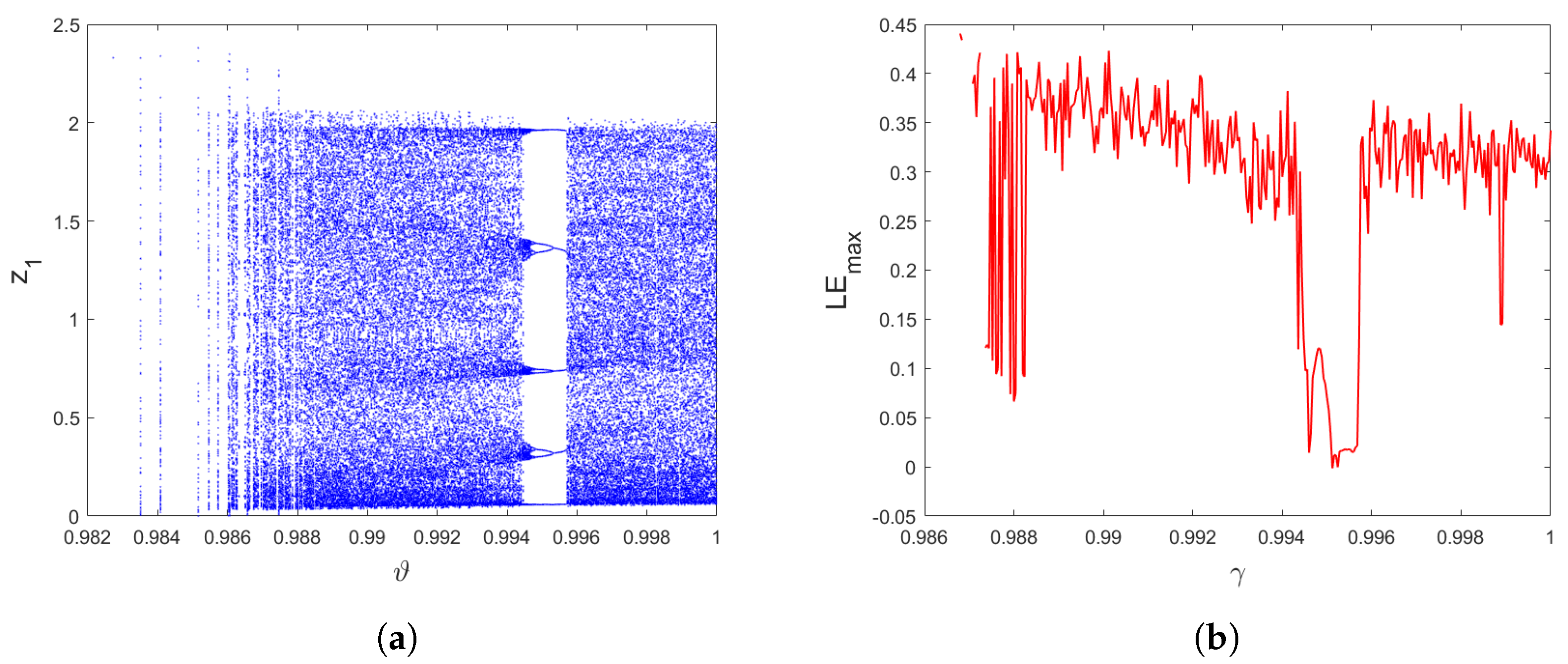
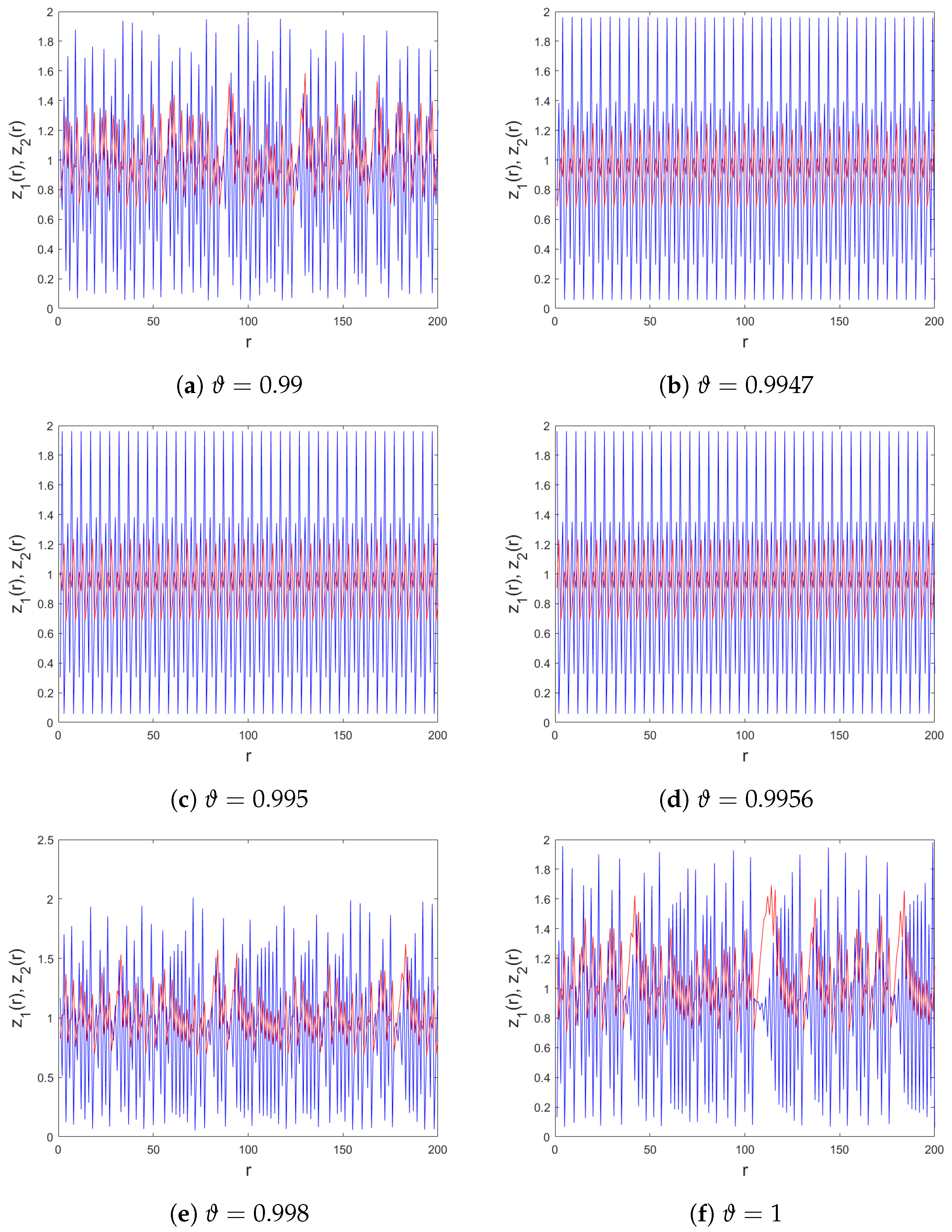
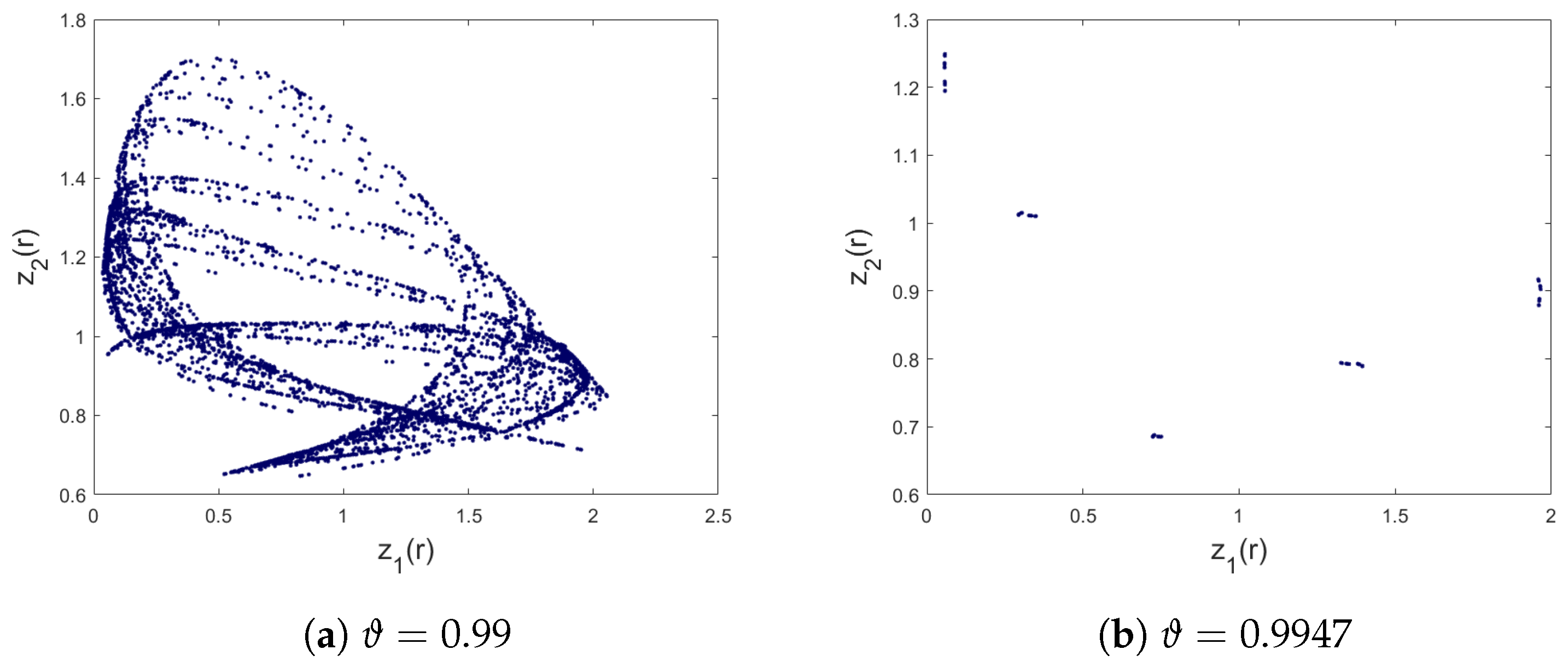
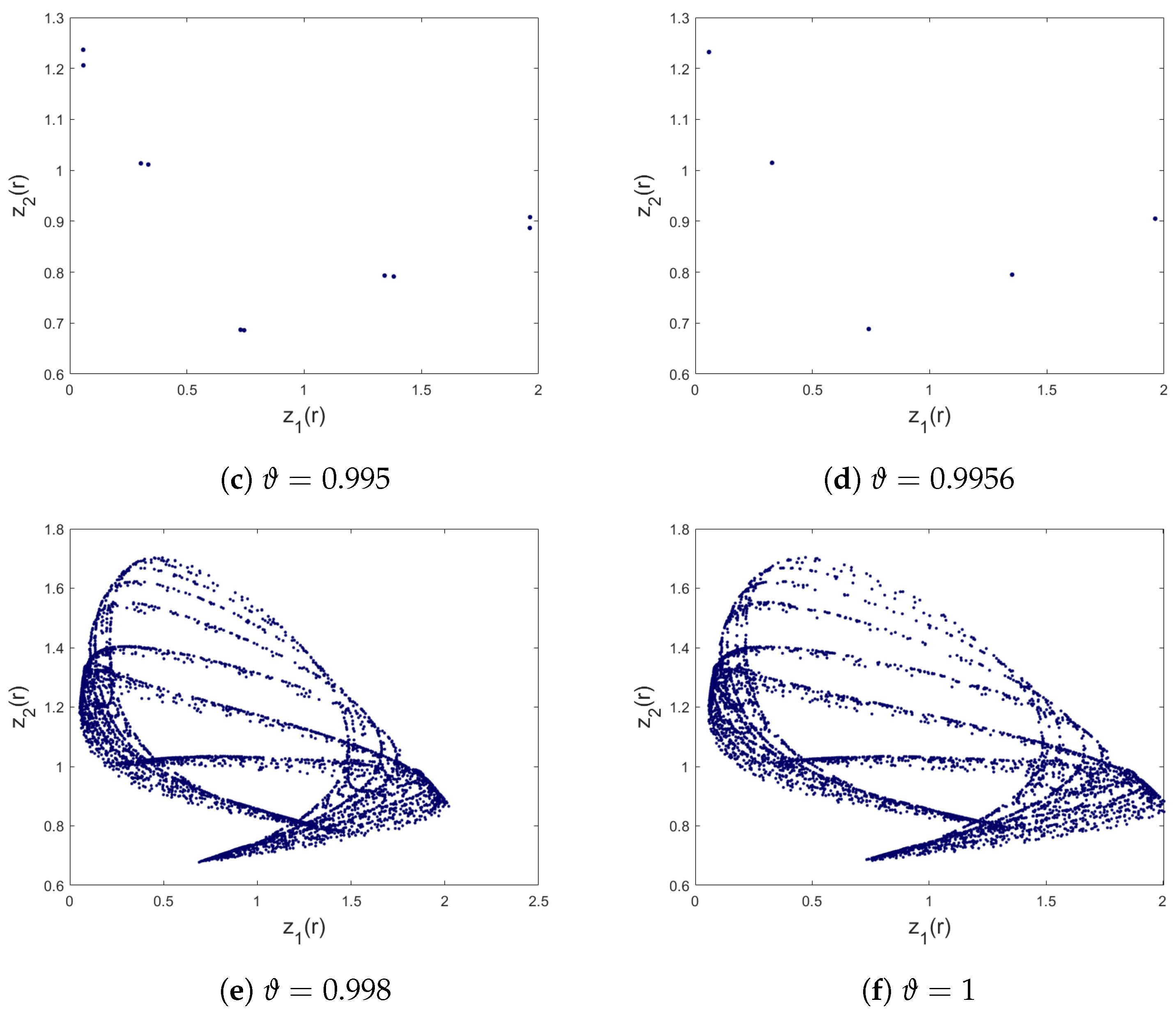
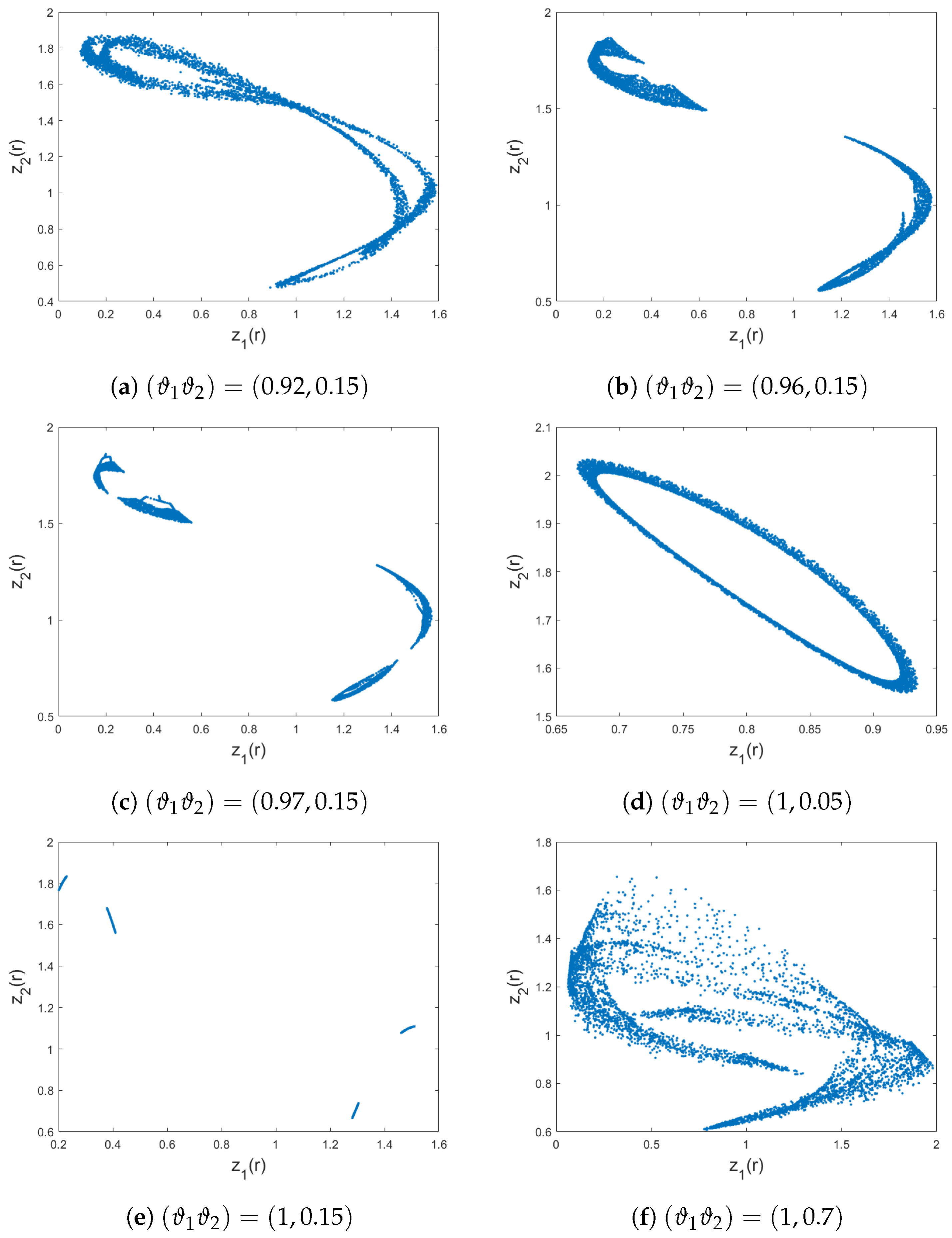
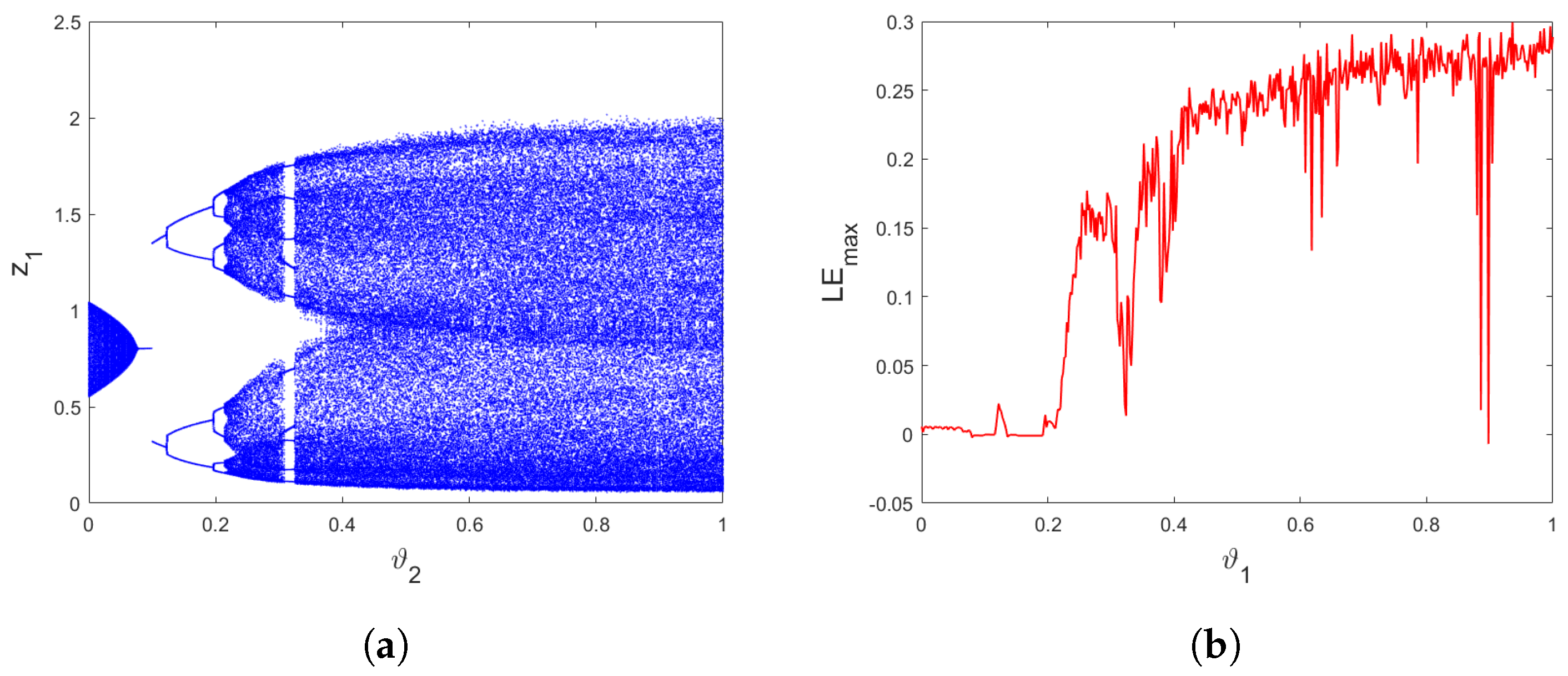
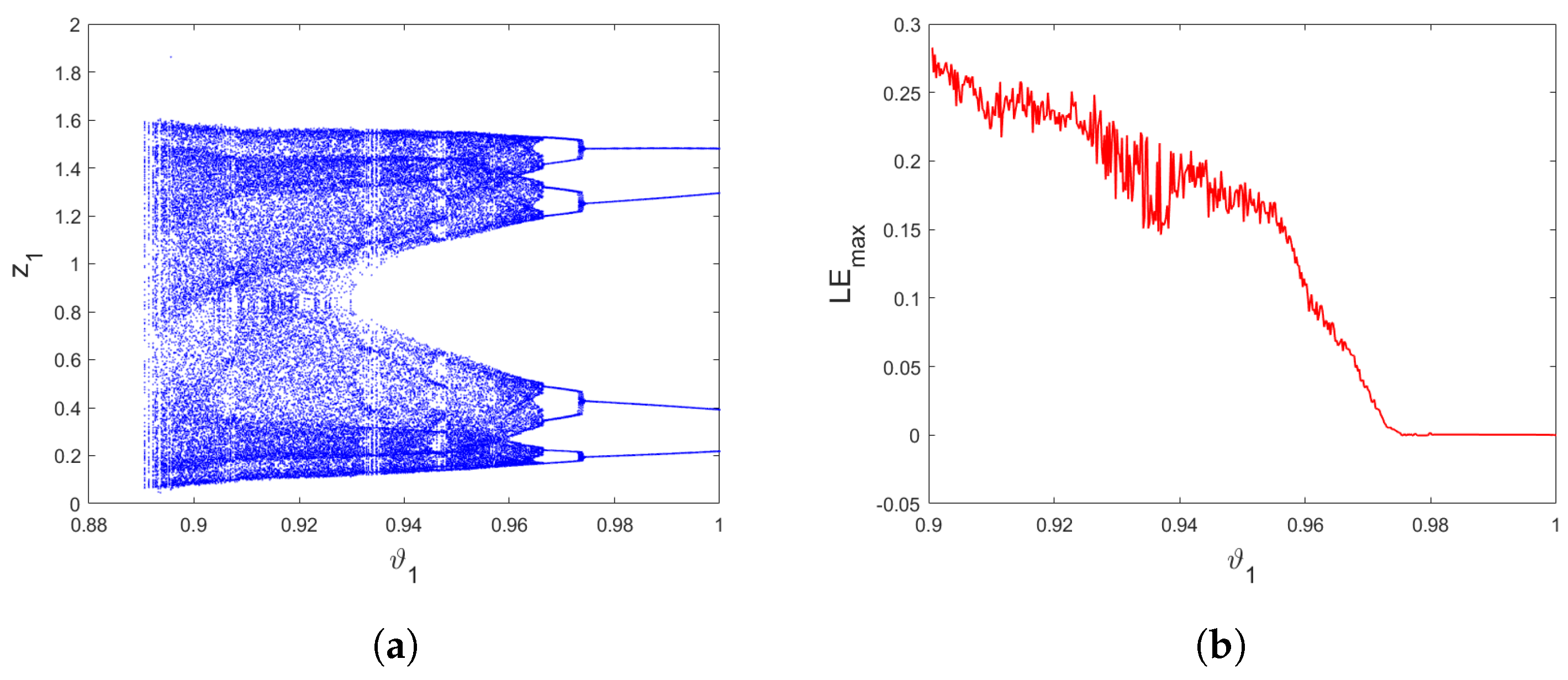
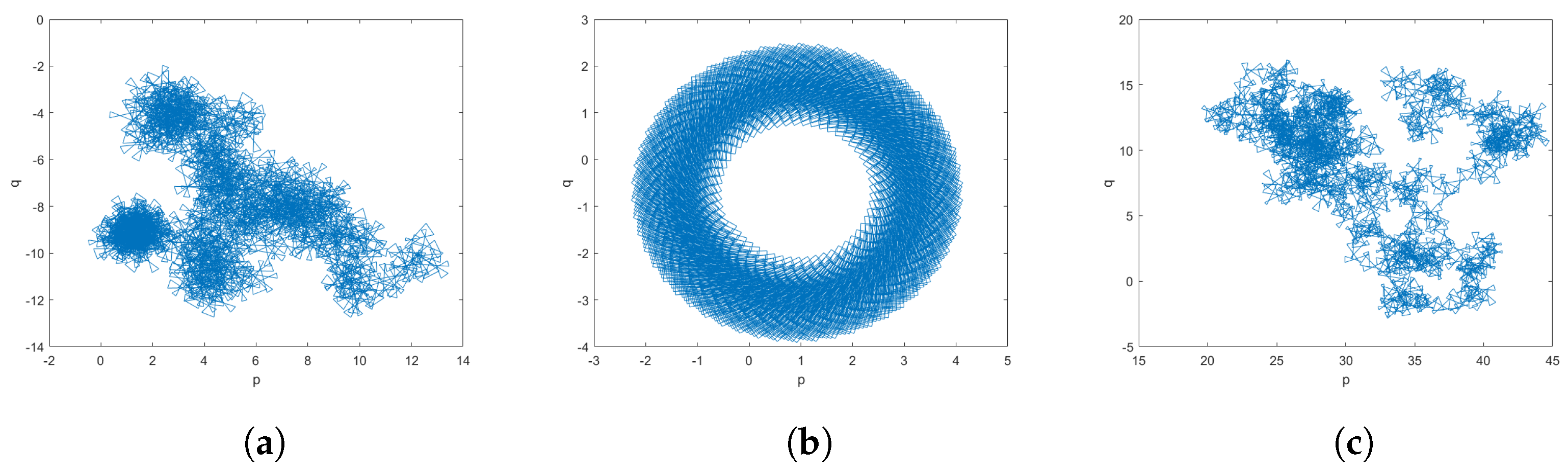
3.2. Incommensurate Fractional Discrete System

In this section, the focus is on studying the dynamics of a fractional discrete-time predator–prey Leslie–Gower system with incommensurate fractional orders. An incommensurate order system involves assigning unique fractional values to each equation in the model. Therefore, the discrete system can be expressed as an incommensurate fractional discrete predator–prey Leslie–Gower model with an Allee effect on the predator population as follows:

$$\begin{array}{cc}\hfill {}^c{\Delta }_a^{{\vartheta }_1}{z}_1\left(r\right)& =z_1(r+{\vartheta }_1-1)exp\left[{\delta }_1-\alpha z_1(r+{\vartheta }_1-1)-\frac{h_1{z}_2(r+{\vartheta }_1-1)}{z_1(r+{\vartheta }_1-1)+b}\right]-z_1(r+{\vartheta }_1-1),r\in {\mathbb{N}}_{a-{\vartheta }_1+1}\hfill \\ \hfill {}^c{\Delta }_a^{{\vartheta }_2}{z}_2\left(r\right)& =z_2(r+{\vartheta }_2-1)exp\left[\frac{{\delta }_2{z}_2(r+{\vartheta }_2-1)}{z_2(r+{\vartheta }_2-1)+m}-\frac{h_2{z}_2(r+{\vartheta }_2-1)}{z_1(r+{\vartheta }_2-1)+c}\right]-z_2(r+{\vartheta }_2-1),r\in {\mathbb{N}}_{a-{\vartheta }_2+1}.\hfill \end{array}$$

(15)

The numerical formula of the incommensurate fractional discrete-time predator–prey Leslie–Gower model (15), using Theorem 1, is described as:

$$\left\{\begin{array}{c}{z}_1(r+1)=z_1\left(0\right)+{\displaystyle \sum _{k=0}^n}\frac{\mathsf{\Gamma }(r-1-k+{\vartheta }_1)}{\mathsf{\Gamma }\left({\vartheta }_1\right)\mathsf{\Gamma }(r-k)}\left(z_1\left(k\right)exp\left[{\delta }_1-\alpha z_1\left(k\right)-\frac{h_1{z}_2\left(k\right)}{z_1\left(k\right)+b}\right]-z_1\left(k\right)\right),\hfill \\ z_2(r+1)=z_2\left(0\right)+{\displaystyle \sum _{k=0}^n}\frac{\mathsf{\Gamma }(r-1-k+{\vartheta }_2)}{\mathsf{\Gamma }\left({\vartheta }_2\right)\mathsf{\Gamma }(r-k)}\left(z_2\left(k\right)exp\left[\frac{{\delta }_2{z}_2\left(k\right)}{z_2\left(k\right)+m}-\frac{h_2{z}_2\left(k\right)}{z_1\left(k\right)+c}\right]-z_2\left(k\right)\right),r=1,2,\cdots .\hfill \end{array}\right.$$

(16)

To illustrate the impact of the incommensurate order on the behaviours of the fractional discrete-time predator–prey Leslie–Gower model (15), we set the system parameters ${\delta }_1=3.3$, ${\delta }_2=1$, $\alpha =3.3$, $h_1=1.2$, $h_2=0.525$, $b=2.5$, $c=0.5$, $m=0.9$ and I.C $(z_1\left(0\right),z_2\left(0\right))=(1,2)$, Figure 5 shows the resulting phase plots for different incommensurate order. As can be observed in Figure 5, the system (15) displays periodic behaviour for $\left({\vartheta }_1{\vartheta }_2\right)=(0.92,0.15)$ and it displays chaotic behaviour for chosen fractional incommensurate orders. Still, the shape of the attractors differs from one fractional incommensurate orders to another and the attractors are extremely different from those obtained in Figure 4. These results prove that the choice of the fractional incommensurate order influences the shape of the attractors of the system (15).

Since the phase plots are not definitive to describe the nature of the dynamics of the system, we are going to observe the bifurcation and the maximum Lyapunov exponents plots concerning the parameter $m\in [0,1]$ to give more precise details on the dynamics of the system (15). We draw bifurcations and its $L{E}_{max}$ for three different fractional incommensurate orders $({\vartheta }_1,{\vartheta }_2)=(0.96,0.15)$, $({\vartheta }_1,{\vartheta }_2)=(1,0.15)$, and $({\vartheta }_1,{\vartheta }_2)=(1,0.7)$ and with the values ${\delta }_1=3.3$, ${\delta }_2=1$, $\alpha =3.3$, $h_1=1.2$, $h_2=0.525$, $b=2.5$, $c=0.5$, $m=0.9$ and I.C $(z_1\left(0\right),z_2\left(0\right))=(1,2)$ as illustrated in Figure 6. When looking at Figure 6, it is easy to observe that the shape of the bifurcation diagrams is different for the three proposed incommensurate orders. In addition, when we change the value of the incommensurate orders ${\vartheta }_1$ and ${\vartheta }_2$, the stability region shrink and the chaotic region expand.

Furthermore, to gain a more precise understanding of the impact of incommensurate orders on the dynamics of the discrete predator–prey Leslie–Gower model with an Allee effect on the predator population (15), we have fixed ${\vartheta }_1=1$ and generated a bifurcation diagram along with a plot of its $L{E}_{max}$ when ${\vartheta }_2\in (0,1]$ and using the same parameters stated earlier. From Figure 7, we can see that when the incommensurate order ${\vartheta }_2$ close to 0, the trajectories becomes chaotic and the $L{E}_{max}$ values are positive. When ${\vartheta }_2\in [0.138,0.194]$, stable trajectories are obtained with the appearance of the periodic motion with 2, 4 and 8-period orbits. When ${\vartheta }_2$ increases, the trajectories of the suggested incommensurate fractional discrete-time predator–prey Leslie–Gower model (15) gradually evolve from a stable to a chaotic motion by means of period-doubling bifurcation. In addition, if we continue increases ${\vartheta }_2$, another smal periodic window are shonw in the interval ${\vartheta }_2\in [0.32,0.332]$ and when ${\vartheta }_2$ becomes large and close to 1, the incommensurate fractional discrete predator–prey Leslie–Gower model (15) become totally chaotic and the $L{E}_{max}$ takes their highest value.

Next, we draw the bifurcation chart and its $L{E}_{max}$ of the proposed new incommensurate fractional discrete predator–prey Leslie–Gower model (15) versus ${\vartheta }_1\in (0.92,1]$ and we chose the incommensurate orders as ${\vartheta }_2=0.15$. From Figure 8, in contrast to the previous cases, we observe that the trajectories of the incommensurate model are stable when the order ${\vartheta }_1$ takes larger values and approaches 1 in which the values of $L{E}_{max}$ appreoches 0. In addition, when ${\vartheta }_1$ decreases, periodic windows disappears and chaos are observed where the values of $L{E}_{max}$ are positive. If the incommensurate order ${\vartheta }_1$ decrease further, a transition states are observed and when the order continues to decrease, the trajectories converge toward infinity. According to these results, varying in the incommensurate order have an effect on the dynamical properties of a fractional discrete predator–prey Leslie–Gower model with an Allee effect on the predator population (15) suggesting that the system’s behaviors can be more precisely depicted by incommensurate order values.

4. The 0–1 Test for Chaos and the Complexity Analysis of the Model

This section presents an analysis of the complexity of chaotic behaviours as a means of assessing the dynamical characteristics of chaotic models. Specifically, it is observed that as the level of complexity increases, the degree of chaos exhibited by the system also intensifies. The present study assesses the complexity of the proposed predator–prey discrete-time Leslie–Gower model with an Allee impact on the predator population. This evaluation is conducted through the utilization of the approximate entropy test and the $C_0$ complexity algorithm. In addition, we will use the 0–1 method to confirm the chaos within the system.

4.1. The 0–1 Test of the Model

Here, we will employ the 0–1 test approach, which was provided by Gottwald and Melbourne [31], in order to detect the difference between chaotic and regular behaviors in dynamic systems. We take the series data as input, and if the dynamics of the model are chaotic, the output will be close to 1, otherwise, it will be close to 0. Furthermore, we describe the test as follows:

Firstly, by using the time series ${\left(z_1\left(m\right)\right)}_{m=1,\dots ,N}$, we establish the translation variables as follows:

$$p_{\varsigma }\left(k\right)=\sum _{m=1}^k{z}_1\left(m\right)cos\left(i\varsigma \right),q_{\varsigma }\left(k\right)=\sum _{m=1}^k{z}_1\left(m\right)sin\left(i\varsigma \right),k=1,2,\dots ,N.$$

(17)

The $(p_{\varsigma }-q_{\varsigma })$ chart is used to detect whether or not chaotic behaviours of the proposed FDNN model occur. If the trajectories of $p_{\varsigma }$ and $q_{\varsigma }$ are bounded, the dynamical behaviours of the model are regular, but if they indicate Brownian-like behaviour, the system’s dynamics are chaotic. Furthermore, we introduce the mean square displacement formula as follows:

$$M_{\varsigma }\left(k\right)=\frac{1}{N}\sum _{m=1}^N\left[{\left(p_{\varsigma }(m+k)-p_{\varsigma }\left(m\right)\right)}^2+{\left(q_{\varsigma }(m+k)-q_{\varsigma }\left(m\right)\right)}^2\right],k\le \frac{N}{10}.$$

(18)

Finally, we represent the asymptotic growth by:

$$K_{\varsigma }=\underset{k\to \infty }{lim}\frac{log{M}_{\varsigma }}{logk}.$$

(19)

The growth rate $K=median\left(K_{\varsigma }\right)$ allows the distinction between nonchaotic and chaotic motions in the proposed commensurate FDNN model (3). If K is closer to 0, this suggests that the model is not chaotic, whereas if K is closer to 1, the model is chaotic.

To validate the occurrence of chaotic behaviours in the commensurate order fractional discrete predator–prey Leslie–Gower model with an Allee effect on the predator population (3) and the incommensurate fractional discrete predator–prey Leslie–Gower model with an Allee effect on the predator population (15), the results of the $p-q$ plots for different commensurate and incommensurate values are displayed in Figure 9 and Figure 10, respectively. The bounded trajectories depicted in Figure 9b,c and Figure 10b serve as clear that the system in question is periodic. In contrast, Figure 9a and Figure 10a,c display Brownian-like trajectories, confirming the occurrence of chaotic motions in both the commensurate model (3) and the incommensurate model (15).

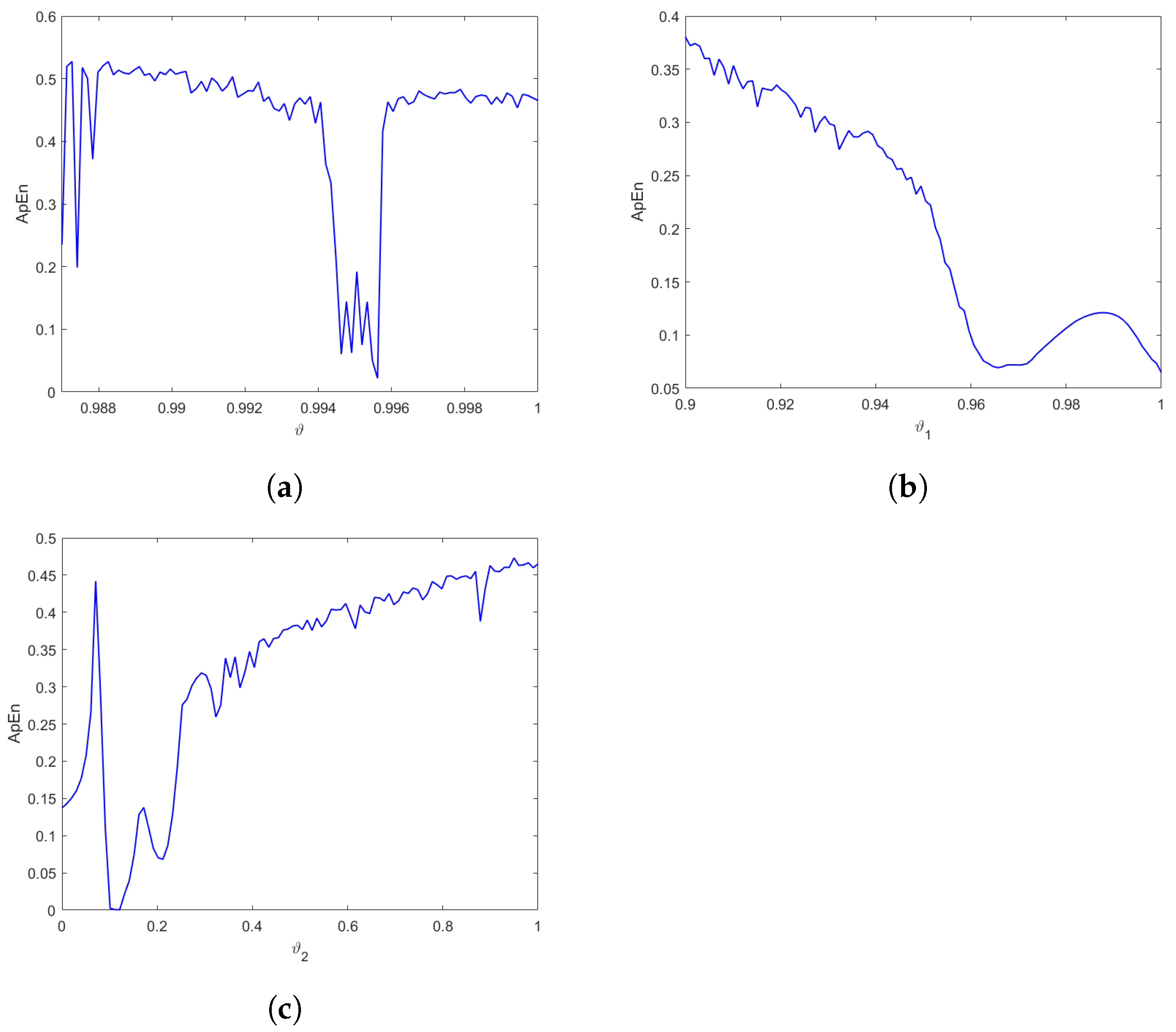
4.2. The ApEn of the Model

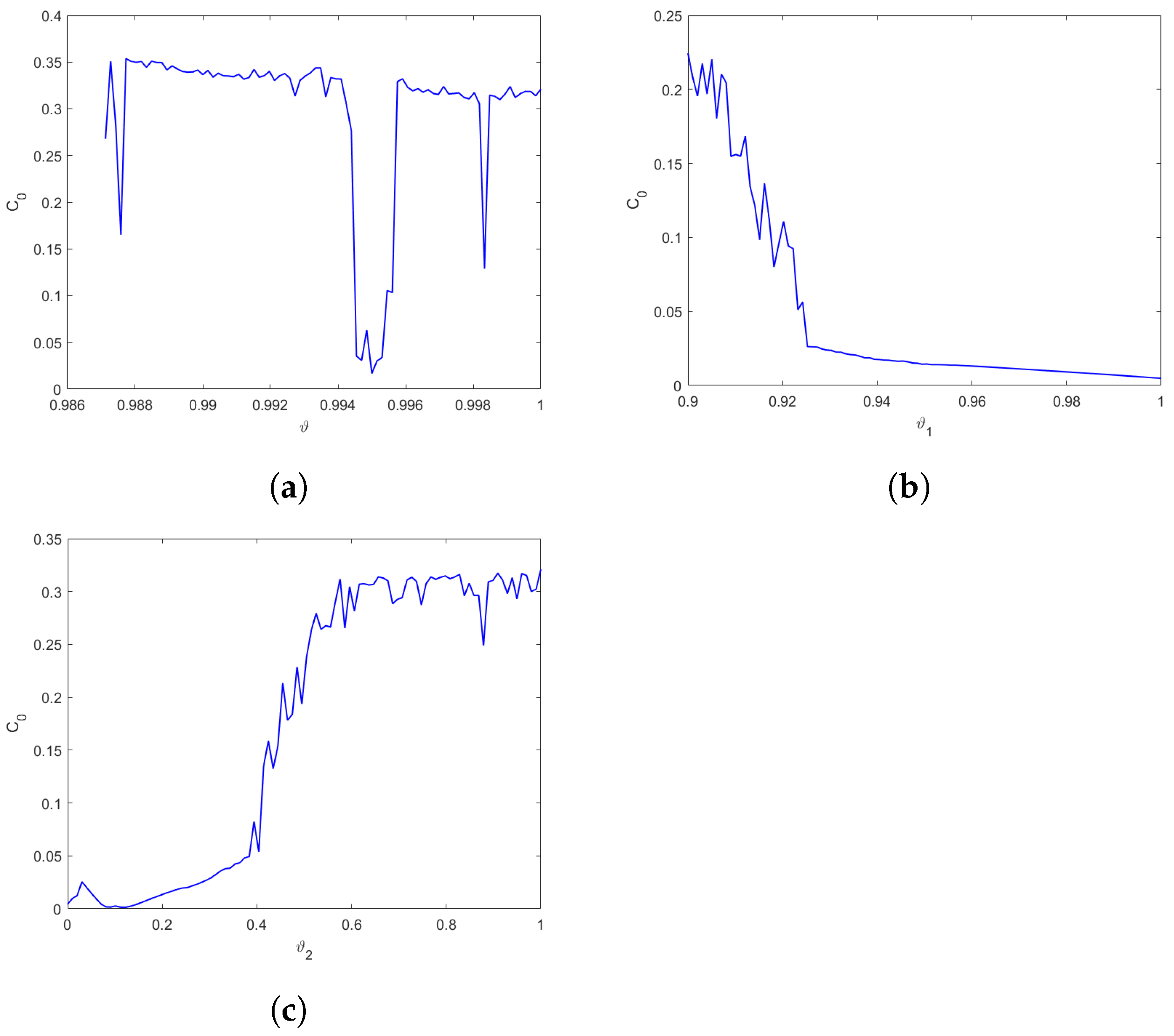
Next, we describe the complexity of the fractional discrete predator–prey Leslie–Gower model with an Allee effect on the predator population (3) by using the approximate entropy (ApEn) algorithm [32]. The ApEn is a measure of the complexity of systems generated by a time series. Note that a time series with a higher value of ApEn are more complex ones. To calculate ApEn, we define first $n-m+1$ vectors as follows:

$$Z\left(i\right)=\left[z\right(i),\dots ,z(i+m-1\left)\right],$$

(20)

for $i\in [1,n-m+1]$ where $z\left(1\right),z\left(2\right),\dots ,z\left(n\right)$ is a set of discrete points. In addition, we describe the following equation:

$$C_i^m\left(r\right)=\frac{K}{n-m+1},$$

(21)

where K is the number of $Z\left(i\right)$ having $d\left(Z\right(i),Z(j\left)\right)\le r$. Note that the value of the approximate entropy depends on two important parameters: the similar tolerance r and the embedding dimension m. Here, we set $m=2$ and $r=0.2std\left(Z\right)$ where $std\left(Z\right)$ is the standard deviation of the data Z. Theoretically, the ApEn is calculated as:

$$ApEn={\varphi }^m\left(r\right)-{\varphi }^{m+1}\left(r\right)$$

(22)

where,

$${\varphi }^m\left(r\right)=\frac{1}{n-m-1}\sum _{i=0}^{n-m+1}log{C}_i^m\left(r\right).$$

(23)

Setting the parameters ${\delta }_1=3.3$, ${\delta }_2=1$, $\alpha =3.3$, $h_1=1.2$, $h_2=0.525$, $b=2.5$, $c=0.5$, $m=0.9$ and I.C $(z_1\left(0\right),z_2\left(0\right))=(1,2)$, the approximate entropy test results of the commensurate fractional discrete predator–prey Leslie–Gower model with an Allee effect on the predator population (3) and the incommensurate fractional discrete predator–prey Leslie–Gower model with an Allee effect on the predator population (15) are shown in Figure 11. It is evident that a time series with greater complexity is necessary to achieve higher ApEn values. Consequently, these results align with the maximum Lyapunov exponents ($L{E}_{max}$) outcomes that were shown before, which therefore validates the existence of chaos in the model under consideration.

4.3. The $C_0$ Complexity of the Model

In this part, we use the $C_0$ complexity method based on the inverse Fourier transform to figure out the complexity of the suggested fractional discrete system. The following is the description of the algorithm [33,34]:

For a sequence $Z\left(0\right),\dots ,Z(N-1)$, the $C_0$ complexity algorithm is given as follows:

1. We compute the Fourier transform of the sequence $x\left(m\right)$ by:

$$Z_N\left(l\right)=\frac{1}{N}\sum _{l=0}^{N-1}x\left(l\right){exp}^{-2\pi i\left(\frac{kj}{N}\right)},l=0,1,\dots ,N-1.$$

(24)

2. We figure out the mean square by: $G_N=\frac{1}{N}{\sum }_{l=0}^{N-1}{\left|Z_N\left(l\right)\right|}^2$ and we define

$${\overline{Z}}_N\left(l\right)=\left\{\begin{array}{cc}{Z}_N\left(l\right)\hfill & \mathrm{if}\parallel Z_N{\left(l\right)\parallel }^2>{rG}_N,\hfill \\ 0\hfill & \mathrm{if}\parallel Z_N{\left(l\right)\parallel }^2\le {rG}_N.\hfill \end{array}\right.$$

(25)

3. We determine the inverse Fourier transform using the following formula:

$$\xi \left(\iota \right)=\frac{1}{N}\sum _{l=0}^{N-1}{\overline{z}}_N\left(l\right){exp}^{2\pi i\left(\frac{\iota l}{N}\right)},\iota =0,1,\dots ,N-1.$$

(26)

4. The complexity of $C_0$ is figured out by using the following formula:

$$C_0=\frac{{\sum }_{\iota =0}^{N-1}\parallel \xi \left(\iota \right)-x\left(\iota \right)\parallel }{{\sum }_{\iota =0}^{N-1}{\parallel x\left(\iota \right)\parallel }^2.}$$

(27)

The $C_0$ complexity of the fractional discrete predator–prey Leslie–Gower model with an Allee effect on the predator population is shown in Figure 12 for ${\delta }_1=3.3$, ${\delta }_2=1$, $\alpha =3.3$, $h_1=1.2$, $h_2=0.525$, $b=2.5$, $c=0.5$, $m=0.9$ and I.C $(z_1\left(0\right),z_2\left(0\right))=(1,2)$ and with different fractional order values, which confirms that the $C_0$ complexity measure the chaos effectively since the obtained results are consistent with the results obtained previously.

5. Conclusions

In this article, we presented a novel two-dimensional fractional predator–prey Leslie–Gower model with an Allee effect on the predator population which is dependent on commensurate and incommensurate orders. The study revealed that the system exhibits intricate and diverse dynamical characteristics. The commensurate and incommensurate fractional order cases are examined using various methods such as plotting phase portraits, creating bifurcation charts, calculating the Lyapunov exponent and using the 0–1 test. Complexity was measured using the ApEn algorithm and $C_0$ test, which confirmed chaos in the model. The results indicate that the proposed model produces chaotic behaviours with a higher complexity degree and a broader range of chaotic regions when fractional orders are varied. Finally, numerical simulations using MATLAB are conducted to verify the findings.

References

1. Ali, I.; Saleem, M.T. Spatiotemporal Dynamics of Reaction–Diffusion System and Its Application to Turing Pattern Formation in a Gray–Scott Model. Mathematics 2023, 11, 1459. [Google Scholar] [CrossRef]
2. Atici, F.M.; Eloe, P. Discrete fractional calculus with the nabla operator. Electron. J. Qual. Theory Differ. Equ. 2009, 3, 1–12. [Google Scholar] [CrossRef]
3. Anastassiou, G.A. Principles of delta fractional calculus on time scales and inequalities. Math. Comput. Model. 2010, 52, 556–566. [Google Scholar] [CrossRef]
4. Abdeljawad, T. On Riemann and Caputo fractional differences. Comput. Math. Appl. 2011, 62, 1602–1611. [Google Scholar] [CrossRef] [Green Version]
5. Hanif, A.; Kashif Butt, A.I.; Ahmad, W. Numerical approach to solve Caputo-Fabrizio-fractional model of Corona pandemic with Optimal Control Design and analysis. Math. Methods Appl. Sci. 2023, 46, 9751–9782. [Google Scholar] [CrossRef]
6. He, Z.Y.; Abbes, A.; Jahanshahi, H.; Alotaibi, N.D.; Wang, Y. Fractional-order discrete-time SIR epidemic model with vaccination: Chaos and complexity. Mathematics 2022, 10, 165. [Google Scholar] [CrossRef]
7. Shatnawi, M.T.; Abbes, A.; Ouannas, A.; Batiha, I.M. A new two-dimensional fractional discrete rational map: Chaos and complexity. Phys. Scr. 2022, 98, 015208. [Google Scholar] [CrossRef]
8. Vignesh, D.; Banerjee, S. Dynamical analysis of a fractional discrete-time vocal system. Nonlinear Dyn. 2023, 111, 4501–4515. [Google Scholar] [CrossRef]
9. Abbes, A.; Ouannas, A.; Shawagfeh, N.; Khennaoui, A.A. Incommensurate Fractional Discrete Neural Network: Chaos and complexity. Eur. Phys. J. Plus 2022, 137, 235. [Google Scholar] [CrossRef]
10. Shatnawi, M.T.; Abbes, A.; Ouannas, A.; Batiha, I.M. Hidden multistability of fractional discrete non-equilibrium point memristor based map. Phys. Scr. 2023, 98, 035213. [Google Scholar] [CrossRef]
11. Abbes, A.; Ouannas, A.; Shawagfeh, N.; Jahanshahi, H. The fractional-order discrete COVID-19 pandemic model: Stability and chaos. Nonlinear Dyn. 2023, 111, 965–983. [Google Scholar] [CrossRef] [PubMed]
12. Batiha, I.M.; Alshorm, S.; Jebril, I.; Zraiqat, A.; Momani, Z.; Momani, S. Modified 5-point fractional formula with Richardson extrapolation. AIMS Math. 2023, 8, 9520–9534. [Google Scholar] [CrossRef]
13. Butt, A.I.K.; Imran, M.; Batool, S.; Nuwairan, M.A. Theoretical Analysis of a COVID-19 CF-Fractional Model to Optimally Control the Spread of Pandemic. Symmetry 2023, 15, 380. [Google Scholar] [CrossRef]
14. Abbes, A.; Ouannas, A.; Shawagfeh, N. The incommensurate fractional discrete macroeconomic system: Bifurcation, chaos and complexity. Chin. Phys. B 2023, 32, 030203. [Google Scholar] [CrossRef]
15. Khennaoui, A.A.; Ouannas, A.; Bendoukha, S.; Grassi, G.; Lozi, R.P.; Pham, V.T. On fractional–order discrete–time systems: Chaos, stabilization and synchronization. Chaos Solitons Fractals 2019, 119, 150–162. [Google Scholar] [CrossRef]
16. Ouannas, A.; Khennaoui, A.A.; Momani, S.; Grassi, G.; Pham, V.T. Chaos and control of a three-dimensional fractional order discrete-time system with no equilibrium and its synchronization. AIP Adv. 2020, 10, 045310. [Google Scholar] [CrossRef]
17. Ouannas, A.; Khennaoui, A.A.; Batiha, I.M.; Pham, V.T. Synchronization between fractional chaotic maps with different dimensions. In Fractional-Order Design; Radwan, A.G., Khanday, F.A., Said, L.A., Eds.; Volume 3 in Emerging Methodologies and Applications in Modelling; Academic Press: Cambridge, MA, USA, 2022; pp. 89–121. [Google Scholar]
18. Saadeh, R.; Abbes, A.; Al-Husban, A.; Ouannas, A.; Grassi, G. The Fractional Discrete Predator–Prey Model: Chaos, Control and Synchronization. Fractal Fract. 2023, 7, 120. [Google Scholar] [CrossRef]
19. Rahmi, E.; Darti, I.; Suryanto, A.; Trisilowati. A modified Leslie–Gower model incorporating Beddington–deangelis functional response, double Allee effect and memory effect. Fractal Fract. 2021, 5, 84. [Google Scholar] [CrossRef]
20. Lin, S.; Chen, F.; Li, Z.; Chen, L. Complex dynamic behaviors of a modified discrete Leslie–Gower Predator–prey system with fear effect on prey species. Axioms 2022, 11, 520. [Google Scholar] [CrossRef]
21. Mondal, N.; Barman, D.; Roy, J.; Alam, S.; Sajid, M. A modified Leslie–Gower fractional order prey-predator interaction model incorporating the effect of fear on prey. J. Appl. Anal. Comput. 2023, 13, 198–232. [Google Scholar] [CrossRef]
22. Yuan, L.G.; Yang, Q.G. Bifurcation, invariant curve and hybrid control in a discrete-time predator-prey system. Appl. Math. Model. 2015, 39, 2345–2362. [Google Scholar] [CrossRef]
23. Ajaz, M.B.; Saeed, U.; Din, Q.; Ali, I.; Siddiqui, M.I. Bifurcation analysis and chaos control in discrete-time modified Leslie–Gower prey harvesting model. Adv. Differ. Equ. 2020, 2020, 45. [Google Scholar] [CrossRef]
24. Din, Q. Complexity and chaos control in a discrete-time prey-predator model. Commun. Nonlinear Sci. Numer. Simul. 2017, 49, 113–134. [Google Scholar] [CrossRef]
25. Khan, A.Q.; Bukhari, S.A.H.; Almatrafi, M.B. Global dynamics, Neimark–Sacker bifurcation and hybrid control in a Leslie’s prey-predator model. Alex. Eng. J. 2022, 61, 11391–11404. [Google Scholar] [CrossRef]
26. Vinoth, S.; Sivasamy, R.; Sathiyanathan, K.; Unyong, B.; Vadivel, R.; Gunasekaran, N. A novel discrete-time Leslie–Gower model with the impact of Allee effect in predator population. Complexity 2022, 2022, 6931354. [Google Scholar] [CrossRef]
27. Allee, W.C. Animal Aggregations, a Study in General Sociology; The University of Chicago Press: Chicago, IL, USA, 1931. [Google Scholar]
28. Aziz-Alaoui, M.A.; Okiye, M.D. Boundedness and global stability for a predator-prey model with modified Leslie–Gower and Holling-type II schemes. Appl. Math. Lett. 2003, 16, 1069–1075. [Google Scholar] [CrossRef] [Green Version]
29. Wu, G.C.; Baleanu, D. Discrete fractional logistic map and its chaos. Nonlinear Dyn. 2014, 75, 283–287. [Google Scholar] [CrossRef]
30. Wu, G.C.; Baleanu, D. Jacobian matrix algorithm for Lyapunov exponents of the discrete fractional maps. Commun. Nonlinear Sci. Numer. Simul. 2015, 22, 95–100. [Google Scholar] [CrossRef]
31. Gottwald, G.; Melbourne, I. The 0–1 test for chaos: A review. In Chaos Detection and Predictability; Springer: Berlin/Heidelberg, Germany, 2016; pp. 221–247. [Google Scholar]
32. Pincus, S. Approximate entropy as a measure of system complexity. Proc. Natl. Acad. Sci. USA 1991, 88, 2297–2301. [Google Scholar] [CrossRef] [Green Version]
33. Shen, E.; Cai, Z.; Gu, F. Mathematical foundation of a new complexity measure. Appl. Math. Mech. 2005, 26, 1188–1196. [Google Scholar]
34. He, S.; Sun, K.; Wang, H. Complexity analysis and DSP implementation of the fractional-order Lorenz hyperchaotic system. Entropy 2015, 17, 8299–8311. [Google Scholar] [CrossRef] [Green Version]
Figure 1. (a) Bifurcation of (3) for  ϑ ( 0 , 1 ) . (b) The corresponding  L E m a x .
Axioms 12 00561 g001
Figure 2. Bifurcations of (3) where  m ( 0 , 1 )  for (a ϑ = 0.99 , (b ϑ = 0.995 , (c ϑ = 0.998 .
Axioms 12 00561 g002
Figure 3. Time evolution of the states of (3) ( z 1 ( r )  (blue line) and  z 2 ( r )  (red line)) for  δ 1 = 3.3 δ 2 = 1 α = 3.3 h 1 = 1.2 h 2 = 0.525 b = 2.5 c = 0.5 m = 0.9  and I.C  ( z 1 ( 0 ) , z 2 ( 0 ) ) = ( 1 , 2 ) .
Axioms 12 00561 g003
Figure 4. Phase portraits of (3) for  δ 1 = 3.3 δ 2 = 1 α = 3.3 h 1 = 1.2 h 2 = 0.525 b = 2.5 c = 0.5 m = 0.9  and I.C  ( z 1 ( 0 ) , z 2 ( 0 ) ) = ( 1 , 2 ) .
Axioms 12 00561 g004aAxioms 12 00561 g004b
Figure 5. Phase portraits of (15) for  δ 1 = 3.3 δ 2 = 1 α = 3.3 h 1 = 1.2 h 2 = 0.525 b = 2.5 c = 0.5 m = 0.9  and I.C  ( z 1 ( 0 ) , z 2 ( 0 ) ) = ( 1 , 2 ) .
Axioms 12 00561 g005
Figure 6. Bifurcation of (15) versus  δ  for (a ( ϑ 1 , ϑ 2 ) = ( 0.96 , 0.15 )  (b ( ϑ 1 , ϑ 2 ) = ( 1 , 0.15 )  (c ( ϑ 1 , ϑ 2 ) = ( 1 , 0.7 ) .
Axioms 12 00561 g006
Figure 7. (a) Bifurcation of (15) versus  ϑ 2  for  ϑ 1 = 1  (b) The corresponding  L E m a x .
Axioms 12 00561 g007
Figure 8. (a) Bifurcation of (15) versus  ϑ 1  for  ϑ 2 = 0.15  (b) The corresponding  L E m a x .
Axioms 12 00561 g008
Figure 9. The  ( p q )  plots of the commensurate fractional discrete predator–prey Leslie–Gower model with an Allee effect on the predator population (3) for (a ϑ = 0.99  (b ϑ = 0.995  (c ϑ = 0.998 .
Axioms 12 00561 g009
Figure 10. The  ( p q )  plots of the incommensurate fractional discrete predator–prey Leslie–Gower model with an Allee effect on the predator population (15) for (a ( ϑ 1 , ϑ 2 ) = ( 0.96 , 0.15 )  (b ( ϑ 1 , ϑ 2 ) = ( 1 , 0.15 )  (c ( ϑ 1 , ϑ 2 ) = ( 1 , 0.7 ) .
Axioms 12 00561 g010
Figure 11. The ApEn of the fractional discrete predator–prey Leslie–Gower model with an Allee effect on the predator population for  δ 1 = 3.3 δ 2 = 1 α = 3.3 h 1 = 1.2 h 2 = 0.525 b = 2.5 c = 0.5 m = 0.9  and I.C  ( z 1 ( 0 ) , z 2 ( 0 ) ) = ( 1 , 2 )  (a) versus  ϑ , (b) versus  ϑ 1  for  ϑ 2 = 0.15 , (c) versus  ϑ 2  for  ϑ 1 = 1 .
Axioms 12 00561 g011
Figure 12. The  C 0  complexity of the fractional discrete predator–prey Leslie–Gower model with an Allee effect on the predator population for  δ 1 = 3.3 δ 2 = 1 α = 3.3 h 1 = 1.2 h 2 = 0.525 b = 2.5 c = 0.5 m = 0.9  and I.C  ( z 1 ( 0 ) , z 2 ( 0 ) ) = ( 1 , 2 )  (a) versus  ϑ , (b) versus  ϑ 1  for  ϑ 2 = 0.15 , (c) versus  ϑ 2  for  ϑ 1 = 1 .
Axioms 12 00561 g012
Disclaimer/Publisher’s Note: The statements, opinions and data contained in all publications are solely those of the individual author(s) and contributor(s) and not of MDPI and/or the editor(s). MDPI and/or the editor(s) disclaim responsibility for any injury to people or property resulting from any ideas, methods, instructions or products referred to in the content.