Article

A Mathematical Model for an Inventory Management and Order Quantity Allocation Problem with Nonlinear Quantity Discounts and Nonlinear Price-Dependent Demand

by
Avelina Alejo-Reyes
1,
Abraham Mendoza
1,*,
Erik Cuevas
2 and
Miguel Alcaraz-Rivera
1
1
Facultad de Ingeniería, Universidad Panamericana, Álvaro del Portillo 49, Zapopan 45010, Mexico
2
Departamento de Electrónica y Computación, Universidad de Guadalajara, CUCEI, Av. Revolución 1500, Guadalajara 44430, Mexico
*
Author to whom correspondence should be addressed.
Axioms 2023, 12(6), 547; https://doi.org/10.3390/axioms12060547
Submission received: 19 April 2023 / Revised: 26 May 2023 / Accepted: 27 May 2023 / Published: 1 June 2023
(This article belongs to the Special Issue Applied Mathematical Modeling and Optimization)

Abstract

:
This article focuses on solving the order quantity allocation problem for retailers. It considers factors such as quality constraints, nonlinear quantity discounts, and price-dependent demand. By formulating it as a nonlinear maximization problem, the article aims to find the best combination of suppliers and order quantity out of infinite solutions to maximize the retailer’s profit. The main contribution of this research is a new mathematical model that can solve the problem of quality constraint and demand in a single step. This problem is complex due to the number of equations, their nonlinear nature, and the various trade-offs given by the market. Additionally, this research considers demand as output and includes price-dependent demand, which is more realistic for retailers. The proposed model was tested using an example from the recent literature and showed better results than the previously published best solution regarding profit maximization.

1. Introduction

Efficient inventory management is crucial for large companies and retailers as it directly affects profitability [1,2]. A retailer’s profits rely on factors such as the cost of purchasing items, the selling price, and the number of items sold in a given period. Therefore, to maximize profits, retailers can increase the number of items sold, the difference between the purchasing and selling costs, or both.
This study focuses on the Economic Order Quantity (EOQ) problem, which involves choosing the appropriate supplier, selecting the order size or percentage of total demand, and determining the order cycle. The EOQ problem can optimize two problems: minimizing costs for manufacturing companies with predetermined production quantities or maximizing profits for final retailers with unpredictable demand. This article belongs to the second group, where the selling price is determined in a single step during problem-solving. This approach is ideal for elastic markets where demand is price-sensitive.
These types of problems can be complex due to various factors, including the number of equations, the nonlinear nature of the problem, and market trade-offs. For example, a single supplier may suffice if supplier capacity exceeds demand, resulting in a relatively simple solution. However, multiple suppliers may be required if demand exceeds capacity, leading to a more complex optimization model. Additionally, discounts offered by suppliers for purchasing larger quantities can add complexity to the problem.
When making decisions, quality is a crucial factor to consider. A study by Mendoza and Ventura [3] defined quality as the “perfect rate”, which is the percentage of items from a supplier that meet all quality standards. For example, a supplier with a perfect rate of 0.98 means that two out of every one hundred items supplied are non-conforming. This affects the total cost, as high-quality suppliers may have higher prices. However, sometimes suppliers with lower perfect rates may be preferred if the cost per item offsets the losses. It is important to note that how defective items are handled may differ from company to company, and this article assumes that the retailer must absorb the cost of defective items without any refunds.
Purchasing is a vital but complicated part of the supply chain. It involves selecting suppliers, determining the number of items to order from each supplier, and deciding how long the order cycle should be. A new mathematical model was introduced in [4] that addresses these challenges recently. This model, referred to as the previous model, considers the demand as output and considers the selling price.
Numerous investigations have been conducted to enhance inventory management. Some of these studies factor in demand as a variable that relies on other parameters or variables. For instance, stock-dependent demand [5,6] assumes that many customers are enticed by the availability of large stock quantities with a wide range of diversity. This can be applied to supermarkets or super-shops. On the other hand, alternative studies postulate that customers are attracted by lower selling prices, which applies to retailers specializing in particular products. Our work belongs to this second category, where demand is price-dependent.
The relationship between demand and selling price can be explained as a trade-off. Retailers have some freedom to choose the selling price. While selling items at a high price may seem logical to make a significant profit, the retailers may not be able to sell the products if the price is too high. There has been research on the mathematical relationship between demand and selling price in the literature [7,8,9,10].
This paper assumes that the retailer buys and sells the same number of items each month, which is crucial for planning and avoiding losses. If the retailer purchases more items than they sell, they can compensate by buying fewer items the following month, but this incurs a stock cost and does not change the average monthly demand. On the other hand, if the retailer fails to meet demand due to purchasing fewer items from the supplier(s), it causes losses and is unacceptable in the decision-making process.
This study examines the impact of a quality constraint, nonlinear quantity discounts on purchasing cost, and a nonlinear price-dependent demand on a retailer’s profit. The demand equation used is the same as in a previous study for easy comparison. The goal is to propose a new mathematical model that improves the retailer’s profit compared to the previously published solution. The problem is formulated as a nonlinear maximization problem that aims to maximize a retailer’s profit by choosing a combination of suppliers and ordering quantities. The article’s main contribution is a new mathematical model that solves the quality constraint and demand in a single step, which is a significant advancement. The problem is complex due to several factors, including nonlinear equations, market trade-offs, and price-dependent demand. Furthermore, unlike previous research, demand is considered an output rather than a given parameter. The proposed model was tested against a recent example from the literature and resulted in a better profit-maximizing solution than the previously published best solution.
The proposed model is solved in MATLAB with the particle swarm optimization (PSO) algorithm because commercial software such as Lingo may not be efficient for such complex problems. To simplify the comparison of results, the numerical example was taken from the state-of-the-art literature. The results showed that the proposed model satisfactorily maximized the benefits while meeting all constraints.
This article is organized as follows: Section 2 provides a literature review on how other works have addressed demand and its relationship to the selling price. Section 3 introduces the problem and its feasibility conditions. Section 4 presents the proposed model and the metaheuristic used to solve the problem. Section 5 analyzes the results, and Section 6 presents the conclusions.

2. Literature Review

This topic has been studied extensively by various authors. Whitin [11] first connected inventory theory and economic price theory by examining how demand is affected by product price. He found that suppliers can offer price discounts to incentivize larger orders. References [12,13] explored how suppliers can offer optimal quantities with quantity discounts. Later, models were developed to determine lot size and optimal price for purchasing a product with all-unit quantity discounts [12,13]. Other researchers have extended the relationship between demand and selling price to include time in their analysis [14,15]. Additionally, supplier selection has been studied with uncertain demand, quantity discounts, and fixed costs [16].
Pricing policies and optimal replenishment schedules have also been explored [17]. Maiti and Giri [18] looked at this topic in a two-echelon supply chain, while others have examined it as a means of coordinating supplier selection and order quantity allocation [19,20,21].
Finally, some researchers have analyzed lot-sizing decisions with price-sensitive demand, including exploring all-quantity discounts to generate an optimal lot-sizing decision [22,23,24,25]. Recent studies have also looked at product demand sensitivity variations using discounts and price patterns [26,27,28,29,30].

3. Description of the Problem and Its Analysis

This section will discuss the problem under study and provide some parameters for a numerical example. Our goal is to help retailers maximize their profits by focusing on a single item that can be purchased from various suppliers. It is worth noting that the optimization algorithm can be run multiple times, depending on the number of items being considered.
Table 1 shows the notation that will be used to describe the problem.
As a retailer, it is important to maintain inventory levels without any shortages. Therefore, the decision maker must purchase a specific type of item and can choose to buy it from one or more of the n suppliers available. Each supplier has its own setup cost (ki), perfect rate (qi), and capacity (ci), ∀ i = 1, …, n. It is also essential to establish a minimum perfect rate (qa). Please refer to Table 1 for a summary of all the parameters and decision variables.
The cost per unit of the item from different suppliers is based on a quantity discount structure. Three suppliers are considered in this example, and their costs are presented in Table 2, Table 3 and Table 4, respectively. The discount structure for each supplier is shown in their respective tables.
Please refer to Table 2 for the pricing information. If the retailer purchases less than 50 items from Supplier 1, the cost is 9 per item. The setup costs for the three suppliers are as follows: Supplier 1 is $500, Supplier 2 is $250, and Supplier 3 is $450. The perfect rates for each supplier are q1 = 0.92, q2 = 0.95, and q3 = 0.98. Suppose the setup or order cost of $500 is dominant for purchases of a few items. In that case, the average cost can be reduced for purchases of larger quantities due to the volume discount offered by the supplier.
After analyzing the suppliers, we found that supplier 1 has the lowest per-unit costs, but their setup cost is the highest. This is because they prefer to sell in larger quantities. On the other hand, Supplier 3 has the most expensive items, and their setup cost is not low either, but they have the highest perfect rate.
Moving on, we express the relationship between selling price and demand through the function in Equation (1):
D = α P e ,
where α and e are the scaling factor and price elasticity index, respectively. For this article’s numerical example, α is equal to 3,375,000 and e is equal to 3.

3.1. The Previous Model

The total average (monthly) profit is formulated using a mixed-integer nonlinear model and depends upon the order quantity assigned to the selected suppliers. This section briefly explains the model introduced by [4], called hereafter the reference model. The solution to the problem consists of finding the number of orders assigned to each supplier ji during the order cycle and the order size for each supplier Qi.
First, the order cycle period is defined as follows:
T c = i = 1 r R i d = i = 1 r R i α P e = R α P e .
Therefore, the complete mixed-integer nonlinear programming model used as our reference model is as follows:
(Reference Model)
Max             Ζ = α P 1 e 1 R [ α P e i = 1 n j i k i + 1 2 r i = 1 n R i 2 j i v i + α P e i = 1 n R i v i ] .
Subject to:
R i = 1 n Q i j i ,
α P e i n Q i j i R c i ,           i = 1 n
i = 1 n Q i ( q i q a ) j i 0 ,
Q i j = 1 a i u i j Y i j ,           i = 1 n   and   j = 1 a i
Q i j = 1 a i u i , j 1 Y i j ,             i = 1 n   and   j = 1 a i
j = 1 a i Y i j 1 ,               i = 1 n
i = 1 n j i = M ,
j i M ,               i = 1 n
j i 0 ,   integer ,                 i = 1 n
P 0 ,
Q i 0 ,                 i = 1 n
Y i j ( 0 , 1 ) ,               i = 1 n   and   j = 1 a i .
Constraint (4) represents the sum of the total ordered quantities considering all selected suppliers. Constraint (5) confirms that the order quantity per supplier does not exceed the supplier’s capacity. Constraint (6) ensures that the supplier’s average quality level is greater than the minimum acceptable quality of the retailer. Constraints (7) and (8) guarantee that the order quantity per selected supplier is within the correct quantity discount interval. Constraint (9) ensures that an interval per selected supplier is selected. Constraint (10) establishes the maximum number of orders per cycle that can be assigned. Constraint (11) ensures that each selected supplier has a total assigned order less than or equal to the total orders per cycle. Constraint (12) ensures that the total number of orders per supplier is an integer. Constraints (13) and (14) help to control non-negative conditions, and constraint (15) establishes the requirements for the binary variable.
The objective of the Reference Model is to maximize the profit function per time unit. The total profit equals the total sales per time unit, αP(1−e), minus the total cost per time unit. The profit function considers the ordering cost per time unit, holding cost per time unit, and purchasing cost per time unit.
The total ordering cost per time unit is calculated as follows:
Ordering   cost = 1 T c i = 1 n j i k i .
The holding cost per time unit from supplier i is calculated by multiplying the holding cost r by the average inventory level, expressed as
Average   inventory   level = 1 T c ( Q i j i 2 ) .
To incorporate it into the objective function, the average inventory cost is calculated as follows:
Inventory   cost = 1 R ( 1 2 r i = 1 n R i 2 j i v i ) .
Finally, the purchasing cost per time unit is calculated as follows:
Purchasing   cost = 1 T c ( i = 1 n Q i j i v i ) .

3.2. Reference Model’s Analysis: The Feasibility of the Solution Considering a New Focus on the Quality Parameters

To analyze the reference model, we need to measure the demand based on the number of pieces without defects. We can define the demand for perfect items, the number of perfect items required considering the demand, and it can be expressed as the demand multiplied by the minimum perfect rate of the retailer (see Equation (20)):
D a = α P e q a .
The solution will provide the following:
(i) 
The number of orders and the order quantity assigned to each supplier. The number of orders to supplier i is called ji; it is assumed that all orders assigned to a specific supplier are of the same size, and the size of the order assigned to supplier i is referred to as Qi.
(ii) 
The order cycle period is in months. This, along with the number of orders and order quantity, determines how many items are purchased each month or each order cycle (the order cycle is expressed in months, it does not need to be an integer). In other words, this can be used to calculate the demand. Then, it is not necessary to provide the demand explicitly. Notice that the percentage of the demand covered by each supplier is not explicitly provided but can also be calculated.
(iii) 
The selling price. This is also implicit since the demand can be calculated, and the selling price can be determined from Equation (1). Still, it is an important variable. In this work, we will consider it to be part of the solution to the problem.
There are countless solutions available, especially if there are no limits to the order cycle or the number of orders. However, some solutions may lead to lower profits or even losses if the selling price is too low. Before we delve into those details, we must differentiate between feasible and infeasible solutions. An infeasible solution is one where the perfect demand is not met or there is a planned shortage. To avoid this, we must set the selling price based on the demand, ensuring that it matches the established demand and minimum perfect rate. If these values do not match up, it will reduce expected profits, which is essentially the same as a shortage.
To meet the demand, you must purchase a quantity of items that is at least equal to the monthly demand multiplied by the order cycle in months:
i = 1 r j i Q i d T C .
To meet the retailer’s minimum perfect rate, we need a second equation. In other words, the demand can be covered by low-quality suppliers, but we must not only ensure that all the items are in demand but also consider that some items will be defective. We can compensate for this by purchasing more items or shortening the order cycle. Equation (22) tells us no planned shortage will be caused by the quality of items:
i = 1 r R i q i d q a T C .
It is important to ensure that the solutions do not exceed the suppliers’ monthly capacity:
R i T C c i .
A solution is feasible if it meets the requirements of Equations (21)–(23), regardless of the method used to arrive at it or the mathematical model. The monthly profits are another parameter that needs to be assessed.

4. The Proposed Model

4.1. Model Analysis

We have presented a revised version of the reference model in Section 3.2. This update aims to expand the range of solutions that can be examined using the reference model, potentially leading to improved outcomes, as evidenced in the results section. It is important to note that the original reference model only accounted for the traditional order cycle period Tc:
T c = i = 1 n Q i j i α P e .
Additionally, the reference model is subject to several constraints. Recall the quality constraint is as follows:
i = 1 n Q i ( q i q a ) j i 0 .
This formulation ensures that the quality of selected suppliers is greater than or equal to the minimum acceptable quality of the retailer qa.
The perfect rate from each supplier (Equation (25)) presents a lack of possibility of finding a solution in scenarios when the perfect rates of suppliers will be less than the minimum acceptable quality. For instance, let us consider the suppliers in the numerical example with perfect rates of 0.92, 0.95, and 0.98, respectively. However, let us consider that the retailer establishes 0.99 (instead of 0.95) as a minimum acceptable quality and the order quantity per supplier is 1000 units within one order. A feasible solution cannot be found:
Q 1 j 1 ( 0.92 0.99 ) + Q 2 j 2 ( 0.95 0.99 ) + Q 3 j 3 ( 0.98 0.99 ) 0 .
Since Qi and ji are positive numbers, no combination can satisfy Equation (26). Since this situation (low perfect rate situation) might be possible in real life, it is highly desirable that models can deal with it. An intuitive solution would be to shorten the order cycle to have more items to compensate for the number of imperfect items and satisfy the demand. Then, a new equation to calculate the order cycle may be required.
If the model allows purchasing more (or the same quantity in a shorter time), the lack of perfect items can be compensated. For example, if a retailer requires 1000 pieces a month and establishes a 0.99 minimum acceptable quality, the company needs 990 perfect pieces each month. Even the lower perfect rate supplier can provide them if 1077 pieces are ordered with a perfect rate of 0.92, resulting in 990.84 perfect parts.
One of the main differences in this article is the reformulation of the order cycle, considering the perfect rate. Let us consider the order quantity per supplier with the required quality as Qijiqi, and the total ordered quantity from supplier i as follows:
R = i = 1 n Q i j i q i .
Demand is calculated as shown in Equation (28), where the minimum acceptable quality of the retailer is considered:
D q a = α P e q a .
Then, the order cycle can be formulated as follows:
T c = i = 1 n Q i j i q i α P e q a .
One of the key components of this work is the reformulation of the order cycle process. Quality parameters are now included in the calculation of the order cycle, rather than being treated solely as constraints. Our proposed model has been shown to yield higher profits than the reference model. Table 5 provides a comparison of various works on the EOQ/EPQ problem using traditional order cycle calculations.
In Table 6, a comparison is made between works using traditional order cycle calculation and quality parameters. All the works listed in Table 5 and Table 6 use nonlinear models, with most of them considering demand as a dependent function based on production cost, stock, or price. Specific works consider all quantity discounts in purchasing costs. Analytic methods and geometric programming are used to find solutions in many works, but this paper explores the use of metaheuristic methods as a fast and efficient alternative. The novelty of this work lies in considering quality parameters as part of the order cycle and demand as a function of price, as shown in Table 5 and Table 6.

4.2. Reformulated Model

After incorporating the redefinition of the order cycle into the reference model, the reformulated model is as follows:
Max             Ζ = α P 1 e 1 i = 1 n Q i j i q i [ α P e q a i = 1 n j i k i + 1 2 r i = 1 n R i 2 j i v i + α P e q a i = 1 n R i v i ] .
Subject to:
α P e q a i n Q i j i R c i ,       i = 1 n
Q i j = 1 a i u i j Y i j ,             i = 1 n   and   j = 1 a i
Q i j = 1 a i u i , j 1 Y i j ,             i = 1 n   and   j = 1 a i
j = 1 a i Y i j 1 ,                 i = 1 n
i = 1 n j i = M ,
j i M ,                     i = 1 n
j i 0 ,   integer ,           i = 1 n
P 0 ,
Q i 0 ,                   i = 1 n
Y i j ( 0 , 1 ) ,               i = 1 n   and   j = 1 a i .
The profit function considers the ordering, holding, and purchasing costs per time unit. The order cycle is calculated using Equation (29). The total ordering cost is expressed as
Total   ordering   cost = 1 T c i = 1 n j i k i .
The holding cost per time unit from supplier i is calculated by multiplying the holding cost r by the average inventory level:
Average   inventory   level = 1 T c ( Q i j i 2 ) .
To calculate the objective function, this is incorporated as
Inventory   cost = 1 R ( 1 2 r i = 1 n R i 2 j i v i ) .
Finally, the purchasing cost per cycle is
Average   purchasing   cost = 1 T c ( i = 1 n Q i j i v i ) .
Constraint (31) ensures that the order quantity per supplier does not exceed the supplier’s capacity. Constraints (4) and (6) are unnecessary in this formulation. Equations (32) to (40) are the same as in the reference model.

4.3. Particle Swarm Optimization (PSO)

The PSO algorithm is used to improve possible solutions by optimizing a function iteratively. This is achieved by adjusting the position and velocity parameters of particles within a search space. The algorithm simulates the behavior of birds and begins by initializing a population of random particles, each representing a possible solution. At each iteration, the particles evolve, and their velocity is updated. The PSO process is further explained using a presentation of the pseudocode.
Pseudocode. Particle Swarm Optimization
P = Po; /*Generating the initial population*/
t = 0;
Repeat
 Update ( p i k and g k );
 Update velocity ( v i k + 1 );
 Update position ( x i k + 1 );
t = t + 1
Until  /*Stopping criteria*/
Output/*Best solution so far*/

4.3.1. Initialization

The algorithm starts by initializing the population. The population represents all the solutions as particles. Decision variables establish particles and are randomly initialized and distributed over the search space of the objective function, following uniform probability distribution. When particles (solutions) are initialized, this decision vector is evaluated in the objective function, and the algorithm calculates the local and global particles. The velocity and position are updated, and particles are modified over iterations.

4.3.2. Velocity of Particles

In order to obtain a new solution vector, the velocity of particles must be updated. This process is based on the local and global influence of the best particles and the last velocity value. The new velocity can be adjusted using the cognitive (c1) and social (c2) factors. The velocity   v i k of each particle or decision vector x i k is updated by employing Equation (45):
v i k + 1 = v i k + c 1 ( r 1 k ( p i k x i k ) ) + c 2 ( r 2 k ( g k x i k ) ) ,
where the velocity vector of the particle x i k for the next iteration k + 1 is denoted by v i k + 1 . v i k is the current velocity, g k is the global best current particle so far, and p i k is the best local so far (up to the current iteration). Additionally, r 1 k and r 2 k are random uniform values usually in the interval [ 0 ,   1 ] .

4.3.3. Movement of Particles

The particles are changed to their new position. This action allows the exploration of new candidate solutions in the search space. The new position is calculated as shown in Equation (46):
x i k + 1 = x i k + v i k + 1 ,
where   x i k + 1 is the updated position of the particle x i k with its new velocity v i k + 1 .
After the particles are updated, they are evaluated in the objective function. The local and global solutions are updated. The entire process is repeated until the maximum number of iterations is reached.

5. Solution of the Numerical Example

Table 7 introduces the parameters for an illustrative numerical example. Table 2, Table 3 and Table 4 show the item’s per-unit cost from each supplier, respectively.
The experiments are implemented using MATLAB R2017a in a computer with a processor Intel(R) core(TM)[email protected].
The reference solution is the best solution presented in [4], in which several solutions have been presented, but the best of them is j1 = 4, j2 = 9, j3 = 5, Q1 = 608.68, Q2 = 378.74, Q3 = 486.95, and P = 15.84. This solution led to a monthly profit of $4179.91.
To solve the proposed model, we utilized the Particle Swarm Optimization (PSO) algorithm. Our population consisted of 200 individuals (m = 200), and we limited the number of iterations to 300 (kmax = 300). By balancing the number of individuals and iterations, we were able to conduct a thorough search for solutions within a reasonable timeframe. The problem involved nine decision variables, which means that it had nine dimensions (n = 9). Our cognitive and social factors were set at c1 = 2 and c2 = 2, respectively. To ensure accuracy and consistency, we repeated the optimization process 30 times for each metaheuristic algorithm. PSO yielded a total of 30 results, and we have provided a summary of the top 10 in Table 8.
Table 9 shows three solutions to the problem, two of them obtained using the proposed model and the third is the solution presented along with the reference model.
The solutions for the reference model obtained through the PSO strategy to solve the problem are listed in Table 10. It is important to mention that these results are not as good as the ones obtained by the proposed model.
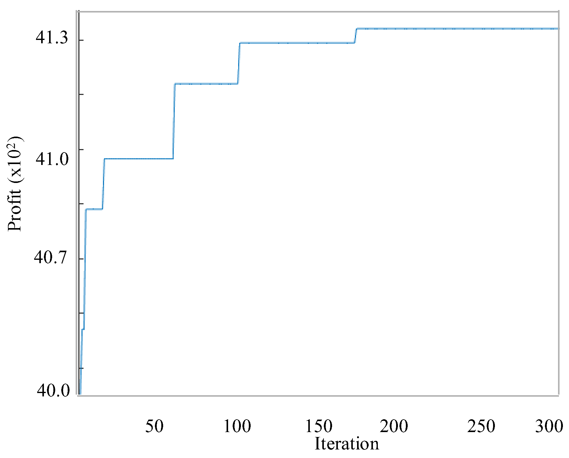
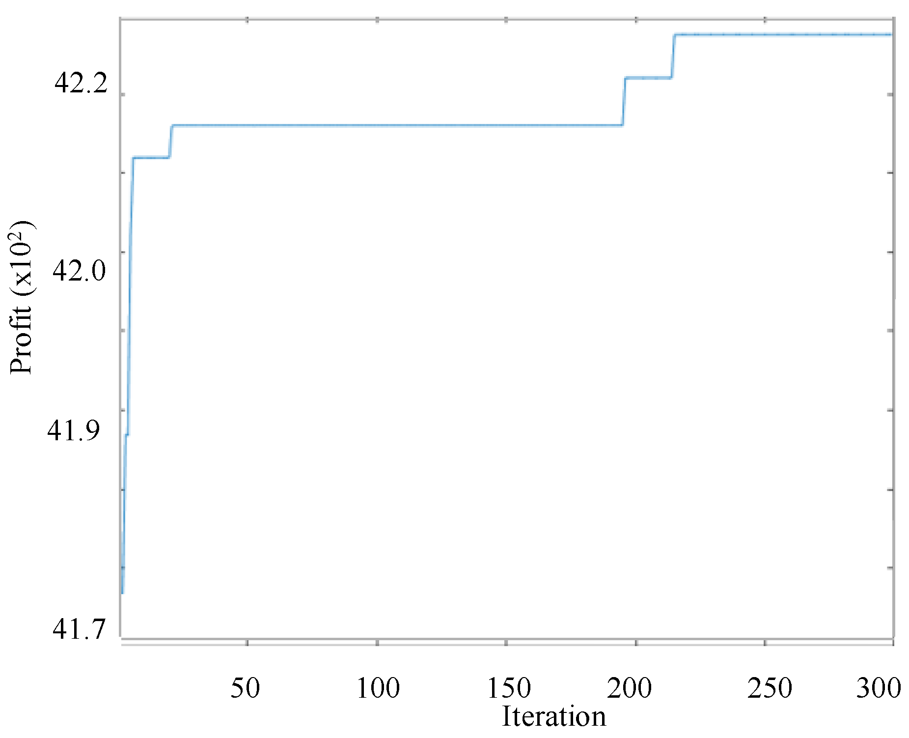
Figure 1 shows that the reference model yields results ranging from $4000 to around $4130, while the new reformulation (see Figure 2) generates results ranging from $4197 to approximately $4235. It is worth noting that all solutions obtained through the proposed model are superior to those obtained through the reference model.

6. Conclusions

This article explores the problem of selecting suppliers and allocating order quantities to maximize profit while considering the effect of the selling price on demand. Previous studies have focused on minimizing inventory costs. Still, this article presents a new mathematical model that includes quality constraints, nonlinear quantity discounts, price-dependent demand, and supplier capacity constraints. The model differs from previous ones in that it considers the perfect rate of suppliers in the order cycle calculation equation and solves the quality constraint in a single step. The Particle Swarm Optimization (PSO) algorithm was used on a numerical example from the literature to test the model. The proposed model outperformed the previous model, leading to a higher profit.

Author Contributions

A.A.-R. and A.M. contributed to the conceptualization of the article; A.A.-R., E.C. and M.A.-R. contributed with the optimization methodology; M.A.-R., E.C. and A.A.-R. contributed with the software and validation; A.A.-R. and A.M. contributed with the formal analysis; A.A.-R. and A.M. wrote the draft and manuscript preparation. All authors have read and agreed to the published version of the manuscript.

Funding

The authors thank the Universidad Panamericana for its support through the internal fund “Fomento a la Investigación UP 2022” under the approved project “UP-CI-2022-GDL-02-ING -Estudio de algoritmos heurísticos y metaheurísticos en la optimización de problemas en la ingeniería” (Study of heuristic and metaheuristic algorithms in the optimization of engineering problems).

Data Availability Statement

Not applicable.

Conflicts of Interest

The authors declare no conflict of interest.

References

  1. Prayag, G. A Study on Inventory Management and Its Impact on Profitability in Foundry Industry at Belagavi, Karnataka. Int. J. Eng. Manag. Econ. 2018, 7, 29–31. [Google Scholar]
  2. Prempeh, K. The Impact of Efficient Inventory Management on Profitability: Evidence from Selected Manufacturing Firms in Ghana; MPRA: Fort Leonard Wood, MO, USA, 2015. [Google Scholar] [CrossRef]
  3. Mendoza, A.; Ventura, J.A. Modeling actual transportation costs in supplier selection and order quantity allocation decisions. Oper. Res. Int. J. 2013, 13, 5–25. [Google Scholar] [CrossRef]
  4. Adeinat, H.; Ventura, J.A. Determining the retailer’s replenishment policy considering multiple capacitated suppliers and price-sensitive demand. Eur. J. Oper. Res. 2015, 247, 83–92. [Google Scholar] [CrossRef]
  5. Pando, V.; García-Laguna, J.; San-José, L.A.; Sicilia, J. Maximizing profits in an inventory model with both demand rate and holding cost per unit time dependent on the stock level. Comput. Ind. Eng. 2012, 62, 599–608. [Google Scholar] [CrossRef]
  6. Khan, M.A.-A.; Shaikh, A.A.; Cárdenas-Barrón, L.E.; Mashud, A.H.M.; Treviño-Garza, G.; Céspedes-Mota, A. An Inventory Model for Non-Instantaneously Deteriorating Items with Nonlinear Stock-Dependent Demand, Hybrid Payment Scheme and Partially Backlogged Shortages. Mathematics 2022, 10, 434. [Google Scholar] [CrossRef]
  7. Khan, M.A.A.; Shaikh, A.A.; Panda, G.C.; Konstantaras, I.; Taleizadeh, A.A. Inventory system with expiration date: Pricing and replenishment decisions. Comput. Ind. Eng. 2019, 132, 232–247. [Google Scholar] [CrossRef]
  8. Liu, L.; Zhao, Q.; Goh, M. Perishable material sourcing and final product pricing decisions for two-echelon supply chain under price-sensitive demand. Comput. Ind. Eng. 2021, 156, 107260. [Google Scholar] [CrossRef]
  9. Ventura, J.A.; Bunn, K.A.; Venegas, B.B.; Duan, L. A coordination mechanism for supplier selection and order quantity allocation with price-sensitive demand and finite production rates. Int. J. Prod. Econ. 2021, 233, 108007. [Google Scholar] [CrossRef]
  10. Hanh, N.T.M.; Chen, J.M.; Van Hop, N. Pricing strategy and order quantity allocation with price-sensitive demand in three-echelon supply chain. Expert Syst. Appl. 2022, 206, 117873. [Google Scholar] [CrossRef]
  11. Whitin, T.M. Inventory control and price theory. Manag. Sci. 1955, 2, 61–68. [Google Scholar] [CrossRef]
  12. Monahan, J.P. Quantity discount pricing model to increase vendor profits. Manag. Sci. 1984, 30, 720–726. [Google Scholar] [CrossRef]
  13. Abad, P.L. Determining Optimal Selling Price and Lot Size When the Supplier Offers All-Unit Quantity Discounts. Decis. Sci. 1988, 19, 622–634. [Google Scholar] [CrossRef]
  14. Bitran, G.; Caldentey, R. An Overview of Pricing Models for Revenue Management. Manuf. Serv. Oper. Manag. 2003, 5, 203–229. [Google Scholar] [CrossRef]
  15. Ahn, H.S.; Gümüş, M.; Kaminsky, P. Pricing and manufacturing decisions when demand is a function of prices in multiple periods. Oper. Res. 2007, 55, 1039–1057. [Google Scholar] [CrossRef]
  16. Zhang, J.L.; Chen, J. Supplier selection and procurement decisions with uncertain demand, fixed selection costs and quantity discounts. Comput. Oper. Res. 2013, 40, 2703–2710. [Google Scholar] [CrossRef]
  17. Herbon, A.; Khmelnitsky, E. Optimal dynamic pricing and ordering of a perishable product under additive effects of price and time on demand. Eur. J. Oper. Res. 2017, 260, 546–556. [Google Scholar] [CrossRef]
  18. Maiti, T.; Giri, B.C. Two-period pricing and decision strategies in a two-echelon supply chain under price-dependent demand. Appl. Math. Model. 2017, 42, 655–674. [Google Scholar] [CrossRef]
  19. Adeinat, H.; Ventura, J.A. Integrated pricing and lot-sizing decisions in a serial supply chain. Appl. Math. Model. 2018, 54, 429–445. [Google Scholar] [CrossRef]
  20. Tiwari, S.; Jaggi, C.K.; Gupta, M.; Cárdenas-Barrón, L.E. Optimal pricing and lot-sizing policy for supply chain system with deteriorating items under limited storage capacity. Int. J. Prod. Econ. 2018, 200, 278–290. [Google Scholar] [CrossRef]
  21. Sutrisno, S.; Sunarsih, S.; Widowati, W. Probabilistic programming with piecewise objective function for solving supplier selection problem with price discount and probabilistic demand. Int. Conf. Electr. Eng. Comput. Sci. Inform. (EECSI) 2020, 7, 63–68. [Google Scholar] [CrossRef]
  22. Wang, F.; Diabat, A.; Wu, L. Supply chain coordination with competing suppliers under price-sensitive stochastic demand. Int. J. Prod. Econ. 2021, 234, 108020. [Google Scholar] [CrossRef]
  23. Lin, Q.; Xiao, Y.; Zheng, J. Selecting the supply chain financing mode under price-sensitive demand: Confirmed warehouse financing vs trade credit. J. Ind. Manag. Optim. 2021, 17, 2031–2049. [Google Scholar] [CrossRef]
  24. Venegas, B.B.; Ventura, J.A. A two-stage supply chain coordination mechanism considering price-sensitive demand and quantity discounts. Eur. J. Oper. Res. 2018, 264, 524–533. [Google Scholar] [CrossRef]
  25. Khan, M.A.A.; Ahmed, S.; Babu, M.S.; Sultana, N. Optimal lot-size decision for deteriorating items with price-sensitive demand, linearly time-dependent holding cost under all-units discount environment. Int. J. Syst. Sci. Oper. Logist. 2020, 9, 61–74. [Google Scholar] [CrossRef]
  26. Siraj, I.; Hassan, M.K.; Maroney, N. Product demand sensitivity and the corporate diversification discount. J. Financ. Stab. 2020, 48, 100748. [Google Scholar] [CrossRef]
  27. Büyükdağ, N.; Soysal, A.N.; Kitapci, O. The effect of specific discount pattern in terms of price promotions on perceived price attractiveness and purchase intention: An experimental research. J. Retail. Consum. Serv. 2020, 55, 102112. [Google Scholar] [CrossRef]
  28. Holguín-Veras, J.; Encarnación, T.; González-Calderón, C.A. User perception of fairness of time-of-day pricing and other typical toll discounts. Transp. Res. Part A Policy Pract. 2020, 137, 560–581. [Google Scholar] [CrossRef]
  29. Jadidi, O.; Jaber, M.Y.; Zolfaghri, S.; Pinto, R.; Firouzi, F. Dynamic pricing and lot sizing for a newsvendor problem with supplier selection, quantity discounts, and limited supply capacity. Comput. Ind. Eng. 2021, 154, 107113. [Google Scholar] [CrossRef]
  30. Shouyu, M.; Zied, J.; Qingguo, B. Optimal pricing and ordering decisions for a retailer using multiple discounts. Eur. J. Oper. Res. 2022, 299, 1177–1192. [Google Scholar]
  31. Moon, I.; Yun, W.Y.; Sarkar, B. Effects of variable setup cost, reliability, and production costs under controlled carbon emissions in a reliable production system. Eur. J. Ind. Eng. 2022, 16, 371–397. [Google Scholar] [CrossRef]
  32. Kugele, A.S.H.; Ahmed, W.; Sarkar, B. Geometric programming solution of second degree difficulty for carbon ejection controlled reliable smart production system. RAIRO-Oper. Res. 2022, 56, 1013–1029. [Google Scholar] [CrossRef]
  33. Pando, V.; San-José, L.A.; Sicilia, J. Profitability ratio maximization in an inventory model with stock-dependent demand rate and nonlinear holding cost. Appl. Math. Model. 2019, 66, 643–661. [Google Scholar] [CrossRef]
  34. Pando, V.; San-José, L.A.; Sicilia, J. A new approach to maximize the profit/cost ratio in a stock-dependent demand inventory model. Comput. Oper. Res. 2020, 120, 104940. [Google Scholar] [CrossRef]
  35. Cárdenas-Barrón, L.E.; Shaikh, A.A.; Tiwari, S.; Treviño-Garza, G. An EOQ inventory model with nonlinear stock dependent holding cost, nonlinear stock dependent demand and trade credit. Comput. Ind. Eng. 2020, 139, 105557. [Google Scholar] [CrossRef]
  36. Subramanian, P.; Ventura, J.A.; Mendoza, A. A serial inventory system with supplier selection and order quantity allocation considering transportation costs. Appl. Math. Model. 2016, 40, 612–634. [Google Scholar]
  37. Mendoza, A.; Ventura, J.A. Estimating freight rates in inventory replenishment and supplier selection decisions. Logist. Res. 2009, 1, 185–196. [Google Scholar] [CrossRef]
Figure 1. Convergence graph using PSO to solve the reference model.
Axioms 12 00547 g001
Figure 2. Convergence graph using PSO to solve the proposed model.
Axioms 12 00547 g002
Table 1. Notation of variables and parameters of the problem.
Parameters
ciMaximum monthly capacity of supplier i (given in units per month)
kiOrdering or setup cost of supplier i (given in dollars per order), ∀ i = 1, …, n.
rStorage or holding cost rate (given in dollars per item per month)
qiPerfect rate of supplier i , ∀ i = 1, …, n.
qaMinimum required perfect rate
viPer unit cost (depends on the order quantity assigned Qi)
MThe maximum number of orders assigned per cycle
Decision Variables
jiThe number of orders assigned to supplier i per order cycle (∑j Jij), ∀ i = 1, …, n.
QiOrdered quantity assigned to supplier i (in units), ∀ i = 1, …, n.
PSelling price
Additional Variables
TcOrder cycle period (in months)
RiThe total number of items ordered to supplier i during the order cycle period (Ri = jiQi), ∀ i = 1, …, n.
dDemand per time unit
Table 2. The per-unit cost of items—Supplier 1.
Supplier 1
IntervalBound (Units)Unit Cost (USD)
10–50 v1= 9
250–100 v1 = 8.9
3100–150 v1 = 8.8
4150–200 v1 = 8.7
5200– v1 = 8.6
Table 3. The per-unit cost of items—Supplier 2.
Supplier 2
IntervalBound (Units)Unit Price (USD)
10–75 v2 = 9.8
275–150 v2 = 9.6
3150–225 v2 = 9.4
4225– v2 = 9.2
Table 4. The per-unit cost of items—Supplier 3.
Supplier 3
IntervalBound (Units)Unit Price (USD)
10–100 v3 = 10.5
2100–200 v3 = 10.4
3200– v3 = 10.3
Table 5. Comparison with other works in the literature.
ReferenceEPQ/EOQDiscountsDemand Depends onMethodologyConsidering Quality
Moon I. et al. [31]EPQNoProduction costGeometric programmingNo
Kugele ASH. et al. [32]SmartNoN.A.Geometric programmingNo
Pando et al. [33]EOQNostockAnalyticNo
Pando et al. [34]EOQNostockAnalyticNo
Cárdenas-Barrón et al. [35]EOQNostockAnalyticNo
Ventura et al. [9]EOQNopriceAnalyticNo
Venegas et al. [2]EOQAll unitspriceGame theoretic modelNo
Adeinat and Ventura [4]EOQAll unitspriceAnalyticYes
This studyEOQAll unitspriceMetaheuristicYes
Table 6. Comparison with works that used quality parameters.
ReferenceQuality Parameters Are Considered asDemand Depends onParameters of the Order Cycle
Mendoza A. et al. [3]Quality constraintConstant Demand, order quantity, number of orders
Subramanian P. et al. [36]Quality constraintConstant Demand, order quantity, number of orders
Mendoza A. et al. [37]Quality constraintConstant Demand, order quantity, number of orders
Adeinat and Ventura [4]Quality constraintPrice Demand, order quantity, number of orders
This studyPart of the order cyclePriceDemand, order quantity, number of orders, quality parameters
Table 7. Parameters of the instance.
VariableNumerical Example Data
r3 suppliers
r0.3 per month
kik1 = 500, k2 = 250, k3 = 450, dollars per order
qiq1 = 0.92, q2 = 0.95, q3 = 0.98
qa0.95
cic1 = 300, c2 = 350, c3 = 250, units a month
α3,375,000
e3
Table 8. Results using Particle Swarm Optimization in the proposed model.
j1j2j3Q1Q2Q3PProfitTc
5100625.2024357.5136017.48964$4195.262810.4658
5100460.4654263.152017.48778$4195.57027.7031
10105447.4173507.6502399.816.40596$4199.64715.0089
490618.4156317.4855017.47399$4200.14968.3043
9100395.3861415.1201017.419$4200.640111.8975
7100481.8841397.9198017.46638$4211.589211.3869
6100517.472372.3754017.48854$4212.087610.6669
7100438.2362361.4035017.46361$4213.366810.3913
5102668.2426387.1903409.394216.84653$4219.427611.2654
6100491.0763346.7467017.43933$4223.26419.9333
351566.374394.1614352.010216.89048$4236.15055.6816
Table 9. Best results using both the previous and the proposed model.
Methodj1j2j3Q1Q2Q3PProfitTc
Proposed6100491.0763346.7467017.43933$4223.269.93
Proposed351566.374394.1614352.010216.89048$4236.15055.68
Reference495608.6800378.7400486.950015.8400$4179.919.74
Table 10. Results using the PSO algorithm in the previous model.
j1j2j3Q1Q2Q3PProfit Tc
3102611.43482302.2221100016.422054$3991.358.9973
242603.3485549.5823631.892717.07176$3998.976.8828
252447.7809252.1053547.720716.58173$4016.194.3924
31051000397.1731603.4291116.259653$4045.1312.7226
410101000598.94822401.1230916.079424$4046.6417.246
41010781.919500.231357.086216.27514$4066.5014.9458
495703.4059377.2035570.51116.5024$4070.8512.0655
697446.8211507.0697464.782616.34089$4085.3113.5725
61010599.3858521.8324370.700315.91724$4133.2014.9621
6108462.4226416.3043368.747115.98633$4134.5511.9691
Disclaimer/Publisher’s Note: The statements, opinions and data contained in all publications are solely those of the individual author(s) and contributor(s) and not of MDPI and/or the editor(s). MDPI and/or the editor(s) disclaim responsibility for any injury to people or property resulting from any ideas, methods, instructions or products referred to in the content.

